Page | 1
Practice-oriented buildability criteria for developing 3D-printable
1concretes in the context of digital construction
2Venkatesh Naidu NERELLAa*, Martin KRAUSEb, Viktor MECHTCHERINEa
3
aInstitute of Construction Materials, Von-Mieses-Bau, 3 O.G., Georg-Schumann-Str. 07, Technische Universität
4
Dresden,01087 Dresden, Germany 5
bInstitute of Construction Management, Nürnberger Ei, 4. O.G., Nürnberger Straße 31A, Technische Universität
6
Dresden, Dresden, Germany 7
* corresponding author, tel.: +49 351 463 35922, fax: +49 351463 37268, e-mail: [email protected]
8
Abstract
9
Buildability, i.e. the ability of a deposited material bulk to retain its dimmensions under increasing 10
load, is an inherent prerequisite for formwork-free digital construction (DC). Since DC processes 11
are relatively new, no standard methods of characterization are available yet. The paper at hand 12
presents practice-oriented buildabilty criteria by taking various process parameters and 13
construction costs into consideration. In doing so, direct links between laboratory buildability tests 14
and target applications are established. A systematic basis for calculating the time interval (TI) to 15
be followed during laboratory testing is proposed for the full-width printing (FWP) and filament 16
printing (FP) processes. The proposed approach is validated by applying it to a high-strength, 17
printable, fine-grained concrete. Comparative analyses of FWP and FP revealed that to test the 18
buildability of a material for FP processes, higher velocities of the printhead should be established 19
for laboratory tests in comparison to those needed for FWP process, providing for equal 20
construction rates. 21
Highlights: 22
Practice-oriented criteria for characterizing buildability are proposed. 23
The applicability of the model in quantifying the economic viability of 3D-printing is 24
demonstrated. 25
Specimen height and time interval are specified as parameters for buildability tests on 26
printable concretes. 27
Proposed buildability criteria are validated by tests on a printable concrete. 28
Variations regarding buildability test specifications for full-width and filament printing 29
techniques are described. 30
Keywords: Digital Construction; 3D-concrete-printing; buildabiltiy, additive manufacturing. 31
1. Introduction and definitions 32
1.1Digital construction and requirements for fresh concrete
33
The processing of cementitious materials is the technological core of modern construction. In 34
recent years numerous new construction techniques based on digitalization and automation have 35
been developed; see e.g. [1–6]. These modern construction processes can be referred to with the 36
generic process title Digital Construction(DC), which denotesautomated additive (or generative) 37
construction with cementitious materials. DC opens a multitude of opportunities and technological 38
Page | 2
• no need for formwork, enabling high geometric flexibility [6,7], 40
• additional functionalities [1,2,6], 41
• considerable reductions in time and cost [5,8], 42
• low dependency on skilled labor, etc. 43
However, the major significance and revolutionary potential of DC reveal themselves in the context 44
of Construction Industry 4.0 since it represents a logical, decisive step arising from the already 45
well-developed tools of digital design and planning (CAD, BIM, etc.) towards digital 46
manufacturing, thus making construction a fully digitalized, seamless process. 47
Two common digital construction techniques are selective material deposition by extrusion and 48
selective binding. The working principles and details of these two approaches are described in more 49
detail in, for example, [3,5], while Figure 1 presents examples of structures produced using these 50
techniques. When it comes to large-scale and on-site applications, extrusion-based techniques 51
appear more suitable; see Figure 1a. The dimensions of the printing device for selective binding 52
techniques must be bigger than those of the target structure [3,5,9]. This is not the case for many 53
extrusion-based DC technologies, as the examples of CONPrint3D [5] and Apis Cor [10] 54
demonstrate. Furthermore, in the case of selective material deposition by extrusion, material is 55
delivered only where it is needed permanently and should, therefore, be sufficiently “buildable”. 56
In contrast, in selective binding techniques the support material surrounding the material to be 57
bonded is crucial to keeping its shape while it is still in plastic state. The need for support material 58
has both positive and negative consequences: structures of any geometrical shape can be produced 59
(positive); see Figure 1b, but all the non-bonded material must eventually be removed (negative). 60
Thus, at this stage the practical application of selective binding techniques seems to be feasible for 61
off-site production of complex elements having relatively small dimensions only. This is one 62
reason why this article focuses exclusively on extrusion-based techniques. Another reason is that 63
due to the mandatory presence of support material, buildability is not really a challenge in the 64
context of selective binding technology. 65
a) b)
Figure 1. Examples of digital construction approaches: a) structural elements produced on-site using selective
66
material deposition by extrusion [4], b) complex structure of Digital Grotesque II produced in a stationary 3D-67
printer using selective binding technique [11] 68
Based on layering technique, extrusion-based DC processes can be classified as full-width printing 69
element, as in CONPrint3D; see Figure 2a. In case of FP the breadth of the extrudate is many times 71
smaller than the breadth of the target element, as in Contour Crafting [1,2,4,12,13] (Figure 2b) or 72
even more pronounced in fine filament approach called Concrete Printing [2,14,15]; see Figure 2c. 73
Consequently, a cross-section of FP elements consists of outer layers (shell/mold) and inner layers 74
or fillings. 75
a) b) c)
Figure 2. a) CONPrint3D technology as example of full-width printing [courtesy: Chair of Construction Machines,
76
TU Dresden], b) Contour Crafting as example of filament printing [courtesy: Contour Crafting], c) Wonder Bench 77
at Loughborough University as example of fine filament printing (photo by V. Mechtcherine) 78
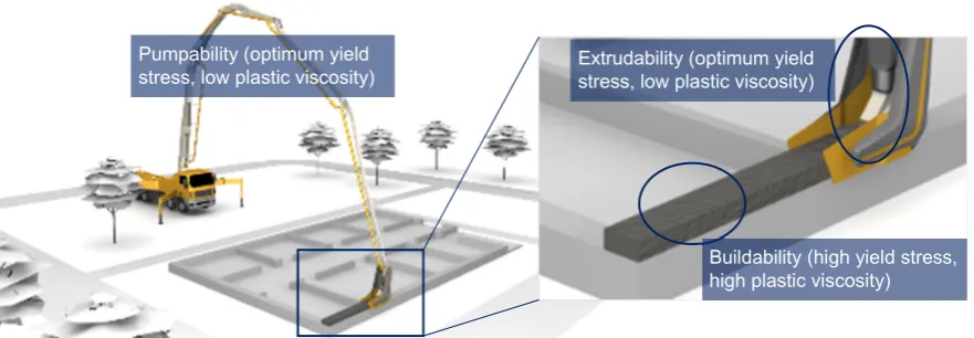
In terms of engineering properties, the primary requirements of cementitious materials for selective 79
material deposition by extrusion are: 1) pumpability, 2) extrudability, and 3) buildability; see also 80
Figure 3. Adequate pumpability should ensure the uninterrupted transportation of fresh concrete 81
and depends on, among other parameters, the plastic viscosity of the concrete, or rather the 82
formation of a lubricating layer [16–18]) in the first place. Extrudability refers to the ease of 83
continuously extruding a material at a given flow rate; it depends on the rheological properties of 84
the fresh concrete and the geometrical configuration of the extruder, or printhead. This being said, 85
buildability, the term and the central subject of this article, is defined as the ability of an extruded 86
material to retain its geometry (shape and size) under sustained and increasing loads. The 87
explanation of this definition follows in Section 1.2. 88
As pointed out in [5], DC is a process of many dualities, e.g. the duality of pumpability and 89
buildability since rheological properties favorable for each of these two processes differ markedly, 90
or the duality arising while determining the ‘rate of printing’, incl. economic efficiency, possible 91
formation of “cold joints”, etc. From a scientific perspective the rheological properties of fresh 92
cementitious material are the most crucial aspect of DC, since they affect not only the process 93
parameters but also the properties of the final product. 94
Figure 3. Illustration of key properties for printable concrete on example of CONPrint3D technology (base sketches 96
are of courtesy: Chair of Construction Machines, TU Dresden). 97
To fulfil the main requirements of extrusion-based DC, cementitious material should be 98
thixotropic, quick setting, quickly hydrating to develop strength very early, and densely packed, 99
and it should possess well controlled rheological properties such as yield stress and plastic 100
viscosity, possibly controllable through internal or external triggers [19]. While this general 101
approach is widely understood, many essential aspects are still under research. The open questions 102
include the systematic choice of rheological parameters and identification of their threshold values. 103
Most importantly, validated experimental methods are necessary to characterize and ensure the 104
desired material properties. In their work in this connection the authors address the question of how 105
one of the primary engineering properties of cementitious materials for DC, namely buildability, 106
can be systematically characterized. Specifically addressed are the questions of what a 107
representative piece of wall is, i.e. height, breadth to be tested in lab-scale buildability tests, and 108
what are the time intervals to be tested in order to call a material printable are addressed. 109
1.2 Buildability requirements and the problem definition
110
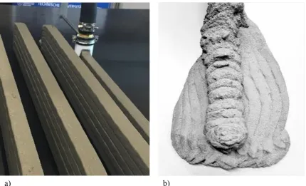
Buildability is the ability of extruded material to retain its geometric dimensions, both shape and 111
size, under sustained or increasing loads. It is a complex, process-specific property which depends 112
not only on material composition, but on process parameters such as layer geometry as well; cf. 113
Figure 2. If buildability, printing rate, printing pattern, and other related aspects are not in harmony, 114
the 3D-printed structure will collapse; see Figure 4b. Buildability depends on, but is not identical 115
to, the structural build-up of cement-based materials, and this dependence is not exclusive. 116
From a practical perspective, there are three primary parameters defining any buildability criteria 117
when applied in laboratory investigations for material characterization: 1) the height of the wall to 118
be printed, 2) the height of each layer or the total number of layers to be printed, and 3) the time 119
interval (TI) between subsequent layers. 120
Since many of the properties required for 3D-printable concretes need a “perfect” balance, it is 121
essential to consider target application at all stages of material development. The buildability-122
defining parameters mentioned above must be carefully determined, considering various 123
theoretical and practical aspects and then applying them in testing the applicability of particular 124
Buildability (high yield stress, high plastic viscosity) Pumpability (optimum yield
mixtures for target DC. 3D-printed elements should have consistent and continuous layer geometry 125
over the entire structure. Figure 4 shows an example of printed specimens with varying numbers 126
of layers and buildabiltiy. It is often appealing to print 10, 20 or as many layers as possible and 127
then ‘designate’ the material as buildable. This trivial approach neither links the material’s fresh 128
properties to the target geometry nor does it consider the economic viability of the target 129
application. While such an approach is still useful for relative comparison of various compositions, 130
printing an arbitrary number of layers with an arbitrary time interval TI is not a reliable method in 131
characterizing buildability. Flowable concrete with low static yield stress, extruded to wide, but 132
thin layers using a long TI,will likely sustain deposition of a higher number of layers in comparison 133
to a less flowable concrete but deposited with a much higher aspect ratio αL,app of individual layers
134
and a short TI; see Section 2. Further relevant parameters are economic viability and durability of 135
the structure, both dependent on TI. Durability is a function of the quality of interlayer joints, which 136
very importantly depends on TI. Thus, for buildability it is crucial to determine one criterion or 137
several criteria based on the intended application and estimated process parameters. 138
In Section 2 previously proposed approaches to estimate buildability based on rheological 139
modelling are critically presented before our own practice-oriented criteria are introduced, which 140
define buildability in terms of target application and process parameters. The applicability of 141
proposed criterion is demonstrated on an example DC process in Section 3, deducing preferable 142
layer height and time interval needed as a basis for developing suitable concretes. Since buildability 143
requirements depend not only upon the target structure but also on the applied printing approach, 144
e.g. massive vs. ‘hollow with sinusoidal cores’ as seen in Figure 2, a corresponding comparative 145
analysis is presented in Section 4. 146
147
Figure 4. a)3D-printed fine-grained concrete specimens (up to five printed layers are depicted here, time interval
148
was 30 s), b) a collapsed printed specimen with buildability deficiency. 149
Page | 6 2. Buildability criteria considering target application
150
2.1 Previous approaches
151
Buildability criteria based on fundamental rheological properties, e.g. static yield stress, and the 152
associated changes over time are still in their genesis; it will take some years until development 153
and validation are complete. Generic rheological models which can consider various process 154
techniques, the shape of the extrudate, and the effects of temperature and other surrounding 155
conditions will take even longer to be formulated and proven. All that existing criteria can predict 156
is whether a deposited material during a time of rest trest deforms or not. However, they do not
157
consider the economic viability of the target application, meaning that even if a material is proven 158
buildable as such at a particular printing rate, it is not known how the use of that particular 159
material/printing rate influences the total economic viability of the target project. Hence, simple, 160
practice-oriented, yet rational buildability-assurance criteria are necessary to accelerate the 161
implementation of digital technologies in construction practice. One such approach is presented in 162
the following sections. 163
In the limited literature on the subject of this article, three significant contributions can be identified 164
[19–21]. In the first on-the-topic, commendable work, Perrot et al. [20] considered the following 165
primary criterion: ‘the flow resistance of a substrate-layer should always be higher than the vertical 166
loads acting on top of it’. The researchers expressed the vertical loads in terms of printing speed 167
and hydrostatic pressure of concrete using Eq. 1: 168
𝜎 = 𝜌 ∙ 𝑔 ∙ 𝑅 ∙ 𝑡 Eq. 1
169
where ρ is the specific weight of concrete, g is the gravity constant, R is rate of construction, and t
170
is the time of construction. 171
The flow resistance of the substrate-layer, expressed as time-dependent static yield stress is 172
described by Eq. 2, Perrot’s exponential evolution model for thixotropy [22]: 173
𝜎 (𝑡) = 𝜏 (𝑡) = 𝛼 𝜏, + 𝐴 ∙ 𝑡 𝑒 − 1 Eq. 2
174
where 𝜏 , and 𝜏 (𝑡) are static yield stresses of the material when resting time is zero and t,
175
respectively; Athix is the constant rate of increase in the static yield stress; tc is a characteristic time
176
after which yield stress evolution at rest becomes exponential; 𝛼 is a geometric factor which 177
depends on the geometry of the deposited layer/printed element [20]. 178
Alternatively, the resistance of a substrate-layer can be estimated using Roussel’s linear evolution 179
model for thixotropy [23]; see Eq. 3: 180
𝜎 (𝑡) = 𝜏 (𝑡) = 𝛼 𝜏 , + 𝐴 ∙ 𝑡 Eq. 3
181
Applying buildability criteria according to Perrot et al. [20] (Eq. 1) for Eqs. 2 and 3, we obtain: 182
𝜌 ∙ 𝑔 ∙ 𝑅 ∙ 𝑡 ≤ 𝛼 𝜏, + 𝐴 ∙ 𝑡 𝑒 − 1 Eq. 4
183
𝜌 ∙ 𝑔 ∙ 𝑅 ∙ 𝑡 ≤ 𝛼 𝜏 , + 𝐴 ∙ 𝑡 Eq. 5
Finally, a critical failure time tfaccording to Perrot with Roussel’ linear model [23] for thixotropy
185 is: 186
𝑡 = ,
∙ ∙ Eq. 6
187
𝑡 predicts at what time after deposition the concrete specimen fails/fractures, if vertical load is 188
increased at rate R and the material initial yield stress 𝜏 , is evolving linearly [23] with a slope
189
Athix.
190
Similar to Perrot et al., Wangler et al. [19] rely on the relationship of flow resistance of a substrate-191
layer, expressed as static yield stress, to the vertical loads acting on top of it. Wangler’s model for 192
minimum time to print a layer follows Von Miese’s criteria and Roussel’ linear model [23] for 193
structural build-up: 194
𝑡 , =√ ∙∙ ∙ Eq. 7
195
In other words, the minimum time 𝑡 , for producing a layer can also be termed as the minimum 196
interval between two successive layers needed to ensure “buildability”. 197
Even though both of these works above are outstanding contributions to the subject of this paper, 198
there are still a few challenges to be mastered before these criteria can become widely applicable. 199
For instance, the parameter 𝛼 is not generically defined yet. Perrot et al. [20] computed 𝛼 200
from the squeeze flow theory of plastics [24,25]. Determining the structuration parameter Athix is
201
also not a trivial task. Currently there are neither standard devices nor standard protocols for 202
characterizing Athixof cementitious materials. Even using most modern rheometers different Athix
203
values may be derived for the same material when different measuring protocols are employed. 204
This implies that for the same material, different critical failure time or minimum time intervals 205
can be computed using Eq. 6 and Eq. 7, respectively. 206
Furthermore, Eq. 6 and Eq. 7 are formulae for the onset of flow/deformation. This means that even 207
if all parameters, including 𝛼 and Athix, are determined precisely, the primary calculation result
208
will be whether the material will deform or not. Such a prediction naturally underestimates the 209
ability of the material to withstand applied loads. In fact, in most practical cases a perfectly rigid 210
layer is not necessary; a layer which deforms within the tolerances allowed is acceptable. An 211
equilibrium reached after few millimeters of deformation is a common possibility as observed in 212
the experiments conducted by the authors and by many other researchers as well. For the target 213
application of the CONPrint3D technology – the construction of residential buildings in Germany 214
– the DIN 18202 "Tolerances in building construction – buildings" [26] specifies the permissible 215
dimensional tolerances and deviations including the specified requirements for the flatness of the 216
wall. When translated for digital construction, i.e. stacking the layers, the DIN 18202 specifications 217
imply that deviations of up to 5 mm between each layer are permissible. Still further, the permitted 218
dimensional deviations from the floor plan depend on the length of the wall. For example, 219
deviations of 12 mm are permitted for a 3 m long wall. These observations, combined with 220
Page | 8 priority to a material which deforms within an allowed limit, as opposed to a perfectly rigid 222
material. 223
More recently, Wolfs et al. [21] developed and validated a numerical model for predicting the 224
failure of 3D-printed concrete. Attributing early strength (0 to 90 min) of printed concrete to 225
“combined inter particle friction and cohesion”, they have adopted Mohr-Coulomb failure criteria, 226
also considering time-dependency [21]. This model does not require measurement of Athix and
227
computation of 𝛼 as in the above-described rheology-based approaches, and the experimental 228
validation of the numerical model showed good qualitative and acceptable quantitative 229
correlations. This approach, however, requires extensive experimental studies and, similar to 230
rheology-based approaches, high precision in execution is needed. In addition, the approach did 231
not address the economic viability of the target application. A simple, practice-oriented criterion 232
for buildability tests has yet to be reported. Note that an extensive review of buildability testing 233
approaches is not the scope of the paper at hand. 234
Process-induced changes in rheological properties is another crucial subject. For example, in the 235
case of pumping SCC, differences in values of yield stress and plastic viscosity were recorded 236
before and after pumping [28]. The variation in rheological properties may result from the “higher 237
shear rates leading to the dispersion of cement particles and depending on available residual 238
superplasticizer in the mixing water” [28]. Additional data on losses in slump, changes of air-void 239
systems, influence of pressure on rheological properties can be found in [29,30]. When it comes to 240
3D-printing based on extrusion on a laboratory scale, even though the material is generally not 241
pumped over large distances, it undergoes high shear rates and is subjected to high pressure in the 242
extruder. Therefore, the exact rheological state of the extrudate may vary depending on the specific 243
extruder and printing-circuit (mixing-transporting-extruding). If large-scale, on-site applications 244
are realized, a pronounced influence of process/pumping on the material rheological state is to be 245
expected. Since rheological properties are usually measured on material taken immediately after 246
mixing, variations of these off-line measured properties in comparison to the actual extrudate 247
rheological properties are inherent. This, however, can be solved by carrying out extensive 248
experimental studies and by the fitting of theoretically predicted “buildability” and experimentally 249
observed “buildability”. To the best of the authors’ knowledge, no such studies have been reported 250
yet. 251
2.2 Suggested buildability criteria
252
The first step in the proposed approach is to identify and define the target application. Based on 253
the building design and project planning, a detailed printing scenario must be established. This task 254
is normally seen as part of the ‘design and process’ aspect of DC work flow. Generally it involves 255
‘slicing’ the 3D geometry, identifying optimum travel route of the printhead, and determining layer 256
breadth, height, and contours. In the case of massive full-width printing (FWP) such as with the 257
CONPrint3D approach [5], layer breadth is equal to final breadth of the wall to be printed; see 258
Figure 3. The criteria presented below are proposed for full-width layer printing. Criteria for 259
filament printing such as the case with Contour Crafting [1] are addressed in Section 4; see Figure 260
For the convenience of further discussion in this article, authors define various relevant aspect 262
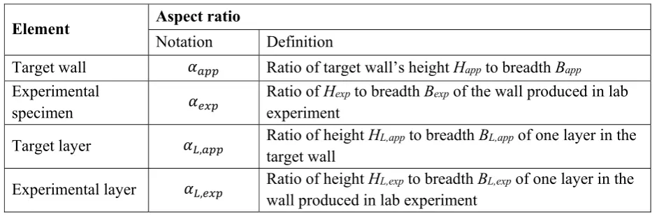
ratios as listed in Table 1. 263
Table 1. Aspect ratios of various elements produced by means of digital construction 264
Element Aspect ratio
Notation Definition
Target wall 𝛼 Ratio of target wall’s height Happ to breadth Bapp
Experimental
specimen 𝛼
Ratio of Hexp to breadth Bexp of the wall produced in lab
experiment
Target layer 𝛼 , Ratio of height HL,app to breadth BL,app of one layer in the target wall
Experimental layer 𝛼 , Ratio of height HL,exp to breadth BL,exp of one layer in the wall produced in lab experiment
265
If the height and breadth of the wall to be printed (part of the target structure) are Happ and Bapp,
266
respectively, then the aspect ratio of the continuously produced “target” element whose buildability 267
has to be ensured can be expressed by Eq. 8: 268
𝛼 = Eq. 8
269
Naturally, the most straightforward but often economically unfeasible manner in verifying 270
buildability is to produce a full-scale structure of the targeted application. Alternatively, 271
buildability can be tested by producing a scaled-down version of the target structure in a laboratory 272
with an appropriate 3D-printing device. In this case printing an arbitrary number of layers with an 273
even so arbitrary time interval TI will, however, not prove a material buildable; see also Section 274
1.2. Thus, the authors propose calculating the minimum height 𝐻 , of the wall to be tested in
275
the laboratory, using the breadth of the layers printed in laboratory experiments 𝐵 and target 276
structure’s aspect ratio 𝛼 (Eq. 8) as: 277
𝐻 , = 𝐵 ∙ 𝛼 Eq. 9
278
If the height of a single layer printed in laboratory experiments is ℎ ,
279
the total number of layers to be printed 280
𝑛 = ,
, Eq. 10
281
Combining, Eq. 9 and Eq. 10 give: 282
𝑛 = ∙
, Eq. 11
283
When downscaling the wall geometry to a laboratory specimen, the limits given by each particular 284
concrete composition must be considered. Specifically, the maximum aggregate of mixtures poses 285
a requirement of minimum breadth and height of each single layer. Choosing the minimum 286
Page | 10 adequate here. Such a ratio ensures that no pronounced wall effects occur so that the features of 288
the material do not change and the material can be well extruded. Further comments on 289
downscaling, including possible changes in maximum aggregate size, follow in Section 2.3. 290
The next open question revolves around determining the time interval between layers TI, which 291
depends on the rate of printing. Rate of printing is a very crucial parameter for formwork-free 292
construction with time-dependent materials such as concrete. If the rate of printing is too high, the 293
printed concrete may not have sufficient time for structural build-up [31] and hence cannot retain 294
its shape and size. If rate of printing is too low, total construction time and costs might become 295
unfeasible. In addition, lower construction rates give rise to so-called “cold joints”, i.e. weak 296
interface bonds between the layers. This leads to the deterioration of both mechanical properties 297
and durability. The time interval TI to be followed in laboratory tests can be deduced directly from 298
the target process parameters. The total travel length L of the printhead can be determined from the 299
layout/floorplan of the target application; see Figure 5. With an average (horizontal) printing 300
velocity of VDC, the minimum time interval between two layers can be expressed as:
301
TImin = L/ VDC Eq. 12
302
In the first approximation VDC is assumed constant, not accounting for a) the acceleration and
303
deceleration at the beginning and the end of printing one layer, respectively, and b) velocity 304
variations when printing corners. For TI > L/VDC, the printing process has to be halted, e.g. to
305
account for possibly insufficient buildability of the applied material, thus leading to longer 306
construction times and losses in efficiency. For TI < L/VDCconcrete buildability is over-engineered,
307
i.e. more than necessary, which may affect the interlayer bond negatively, but also poses greater 308
challenges in meeting the requirements of pumpability and extrudability. While defining TI, the 309
economic viability of the target application/project must be considered as well. The corresponding 310
process term, the average velocity VDC, is already addressed in Eq. 12. It is worthy of note that for
311
a wall of given gross dimensions, the time interval TI will be in the case of FP approaches higher 312
than that for FWP approaches due to longer total travel length of the printhead. This aspect is 313
elaborated in Section 4. For any DC approach to be economically viable, the following condition 314
according to Eq. 13 must be fulfilled: 315
𝐶𝑜𝑠𝑡𝑠 ≤ 𝐶𝑜𝑠𝑡𝑠 Eq. 13
316
where, 𝐶𝑜𝑠𝑡𝑠 and 𝐶𝑜𝑠𝑡𝑠 are the respective total construction costs in the case of the DC 317
approach chosen and in the case of current corresponding conventional construction (CC) 318
approach, respectively. Authors have identified, as an example, replacing masonry structures for 319
residential buildings as the strategic objective for CONPrint3D [5,8]. Therefore, in this case 320
𝐶𝑜𝑠𝑡𝑠 are the current total construction costs for masonry in a unit residential building.
321
Expressing the costs of machine and labor as cost per unit time and material costs as cost per unit 322
volume, the total costs can be estimated by using Eq. 14: 323
(𝑀𝑐𝐶𝑜 + 𝐿𝑎𝐶𝑜 ) ∙ 𝑡 + 𝑀𝑡𝐶𝑜 ∙ 𝑣𝑜𝑙 + 𝐴𝑑𝐶𝑜 ≤ (𝑀𝑐𝐶𝑜 + 𝐿𝑎𝐶𝑜 ) ∙ 𝑡 + 𝑀𝑡𝐶𝑜 ∙ 𝑣𝑜𝑙 Eq. 14
324
where, 𝑀𝑐𝐶𝑜 , 𝐿𝑎𝐶𝑜 and 𝑀𝑐𝐶𝑜 , 𝐿𝑎𝐶𝑜 are the machinery/equipment costs and labor costs 325
Ad𝐶𝑜 are additional costs added only for DC. Additional costs include, among others, costs for 327
concrete curing (more elaborate than usual), additional testing and consulting fees that may be 328
necessary in the case of DC. 𝑡 and 𝑡 are the time needed for constructing the target structure 329
in case of DC and CC, respectively, while voldc and volcc are the total volumes of material used in
330
case of DC and CC, respectively. 331
Expressing time in terms of average velocity in the case of DC and inversed construction rate RI
332
(unit: h/m2) in the case of CC, we obtain:
333
(𝑀𝑐𝐶𝑜 + 𝐿𝑐𝐶𝑜 ) ∙ + 𝑀𝑡𝐶𝑜 ∙ 𝑣𝑜𝑙 + 𝐴𝑑𝐶𝑜 ≤ (𝑀𝑐𝐶𝑜 + 𝐿𝑎𝐶𝑜 ) ∙ (𝑅𝐼 ∙ 𝑠𝑢𝑟𝑓𝑎𝑐𝑒 𝑎𝑟𝑒𝑎) +
334
𝑀𝑡𝐶𝑜 ∙ 𝑣𝑜𝑙 Eq. 15
335
where surface area is the total “one-side” surface area of the element being constructed; 𝐿 is the 336
total travel length of the printhead, which is assumed to be equal to the travel length for a single 337
layer L multiplied by the total number of layers 𝑛 . The traversing of the printhead without 338
printing, for example, to move to a new printing position are not considered here as they are very 339
specific to the target application and the related process parameters. Nevertheless, these can be 340
added to the 𝐿 if known. 341
Additional costs Ad𝐶𝑜 in the case of CONPritn3D are assumed to be a lump sum amounting to 342
10 % of the total construction costs. 343
Rearranging Eq. 15, Eq. 16 for the minimum average printhead velocity for an economically viable 344
DC application can be obtained: 345
𝑉 , ≥ . ∙(( )∙( ∙( ) )∙ ∙ ) ( )∙ Eq. 16
346
Since it is known that: 347
• 𝐿 is equal to the length of the layer multiplied by the total number of layers 𝑛 , 348
• surface area is equal to the length of the layer multiplied by the height of the wall, and 349
• total material volume is the length multiplied by the height and breadth of the walls, 350
Eq. 16 can be transformed to Eq. 17: 351
𝑉 , ≥
( )∙
. ∙(( )∙( ∙ ) ∙ ∙ ) ∙ ∙ Eq. 17
352
where HCC, BCC, HDC, BDC are the height and breadth of the walls in case of CC and DC,
353
respectively. While HCC = HDC is chosen here for ease of comparison, the breadth of the layers
354
produced in DC can be smaller than that of CC. Since materials used for DC applications are often 355
superior to masonry in terms of mechanical performance, thinner walls produced using DC can 356
meet the same design specifications as thicker walls produced using CC. Eqs. 16 and 17 can be 357
adapted also to other DC applications to compute a minimum average printhead velocity that 358
should be attained to make the DC application economically viable with respect to the fabrication 359
process as such. Certainly there are also other factors which may influence the economic feasibility 360
to a great extent. Thus, in general the entire process from planning to actual construction should be 361
evaluated. Specifically, the smooth transition from digital planning to digital fabrication seems to 362
Page | 12
2.3 Additional comments
364
The proposed approach assumes that material behavior tested on the “down-scaled specimens 365
under laboratory conditions (lab-tests)” is representative of the material behavior in “full-scale 366
structure in real application (full-scale)”. In reality differences in material behavior as among the 367
lab-tests and as experienced full-scale may arise, e.g. due to variation in the quality of 368
extrusion/compaction (process-induced changes) or in the evaporation rate related to the volume 369
of printed element. 370
Here it is important to emphasize that the challenge posed by some differences in lab experiments 371
and full-scale applications is a universal issue which is not particular to buildability tests or DC in 372
general. Taken broadly, such issues can only be resolved by full-scale tests and direct comparison, 373
followed by error-minimization measures. The approach proposed in this paper for laboratory tests 374
already takes into account certain considerations in mimicking conditions under full-scale 375
application: 376
a) Tests are performed in-line, i.e. they are integrated in the 3D-printing process, as opposed 377
to offline tests where material has to be collected separately and tested in a test device; thus, 378
time-dependent influences are avoided and errors due to process induced changes are 379
minimized. 380
b) Specimens are extruded using an extruder system similar to that foreseen in the prospective 381
full-scale application, thus subjecting the tested material to similar shear history and degree 382
of compaction. 383
c) The curing of laboratory specimens is adjusted to that planned for the full-scale application, 384
indeed, if planned at all. If specific temperature, humidity, and wind conditions are expected 385
for the full-scale application, the laboratory tests should be performed if possible under 386
similar environmental conditions. 387
d) If admixtures are added in the printhead during full-scale applications, the same procedure 388
should be implemented in the lab-scale 3D-printing. 389
Regarding change of scales, the authors do anticipate that the proposed approach withstand the 390
change in scales, however, with some limitations which need further investigation. So long as the 391
changes are only in dimensions and not in shape of the geometry, the validity of the proposed 392
approach can be seen as convincing. Nevertheless, a correction factor may need to be introduced 393
to take dimensional change into account. Such factors can be identified theoretically/numerically 394
and/or with help of full-scale validation experiments. It goes without saying that in some cases 395
(full-scale applications are large and tall structures) downscaled experiments are the only feasible 396
option to assess the buildability. 397
Another issue is that downscaling is limited by minimum feasible dimensions of layer cross-section 398
and nozzle dimensions as defined by the maximum aggregate size; this is pointed out in Section 399
2.2. To extend the range of downscaling, the maximum aggregate size used in mixtures for 400
laboratory experiments may be reduced. This is an approach used sometimes in the practice of 401
construction for various practical reasons such as the availability of appropriate testing equipment, 402
ease of handling etc. Certainly, such change in material composition must be well thought through, 403
and its consequences must be closely considered. However, it seems feasible to decrease maximum 404
relatively well estimated based on available contemporary knowledge. It is known from [19,20] 406
that the buildability of a printed layer can be expressed in terms of, and proportionally depends on 407
the structural build-up of concrete. MAHAUT et al. [32] related the static yield stress of cementitious 408
suspensions with coarse particles τ (ϕ, t) to the static yield stress of the suspending cement paste 409
τ (0, t), to the time t passed at rest, and to the coarse particle volume fractionφ; see Eq. 19. They
410
suggested that the presence of φ, the volume fraction of coarse particles in a cement paste, will 411
magnify its static yield stress as a function of the volume fraction of coarse particles g(φ). 412
𝜏 (𝜙, 𝑡) = 𝜏 (0, 𝑡)𝑔(𝜙) Eq. 18
413
𝑔(𝜙) = (1 − 𝜙)(1 − 𝜙/𝜙 ) . Eq. 19
414
where 𝜙 is the maximum volume fraction. 415
In addition Mahaut et al. [32] postulated that “the structuration rate Athixhas the same dependence
416
on the coarse particle volume fraction as the yield stress”. Similar models for relating properties 417
of a suspension to suspending paste are presented and discussed in [33–35]. These findings imply 418
that the parameters identified through a proposed approach on a concrete with finer aggregates 419
could be applied to concrete with coarse aggregates using a factor similar to that of Eq. 19. 420
However, this hypothesis is yet to be verified. 421
3. Applying proposed buildability criteria to CONPrint3D
422
Generalized buildability criteria proposed above in Section 2 are applied here to an on-site concrete 423
3D-printing technology, CONPrint3D. On completion of this section, the specifications of 424
buildability tests on cementitious materials applicable for CONPrint3D are clearly derived. As 425
elaborated in Section 2, these necessary specifications are: height of the experimental wall to be 426
printed, number of layers in this wall, and the time interval (TI) between the layers. While the target 427
full-scale implementation of CONPrint3D technology will be primarily with coarse-grained 428
aggregates, of maximum aggregate size 8 mm to 16 mm, the use of fine-grained concrete should 429
not be excluded, certainly not at this stage, since it has many advantages with respect to processing 430
and the maturity of the extrusion machine technology required, “lightness” of the printhead, etc. 431
Thus, as a first step the validation presented below will consider an application case of 432
CONPrint3D where fine-grained concrete is used. The reason behind this is that the validation can 433
be performed directly without need for additional assumptions or specific correcting factors. In a 434
follow up study, the proposed buildability criteria will be applied to 8 mm aggregate, printable 435
concrete, and if necessary adjustment of the approach will be made. Note that the higher material 436
costs of fine-grained concrete are taken into account in Section 3.2. 437
3.1 Height of the wall specimen and number of layers to be tested
438
Of the primary target applications for the CONPrint3D approach, one- to multi-story residential 439
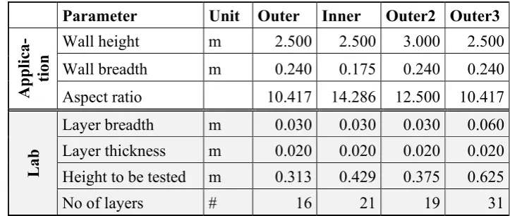
buildings [5,8] make up an important segment; see Figure 5. Table 2 presents the dimensions of the
440
corresponding outer and inner walls for each story. Also presented are the nozzle dimensions 441
employed for the lab-scale 3D-printing testing device (3DPTD), which was designed in 2015 at the 442
TU Dresden and has been used since then for material development. Furthermore, Table 2 presents 443
Page | 14 on how 𝐻 , and 𝑛 vary depending on wall and nozzle dimensions. 𝐻 , and 𝑛
445
are calculated using Eq. 9 and Eq. 11. These calculations highlight the consideration of layer 446
geometry in the proposed buildability criteria. If the laboratory nozzle breadth is increased and 447
laboratory nozzle height remains unchanged, then the height 𝐻 , to be tested in the laboratory
448
also increases. If the thickness of the target wall decreases, as in the case of inner walls, then 449
𝐻 , increases. Similarly, if the height of the printed layer, i.e. nozzle in the lab, increases
450
where its breadth remains unchanged, then the number of layers to be printed in the laboratory tests 451
will decrease. These variations of buildability test specifications are crucial, considering that the 452
nozzle dimensions in the laboratory printers may vary significantly even though the final targeted 453
element (application) dimensions and the geometry of the real-application printhead do not change. 454
455
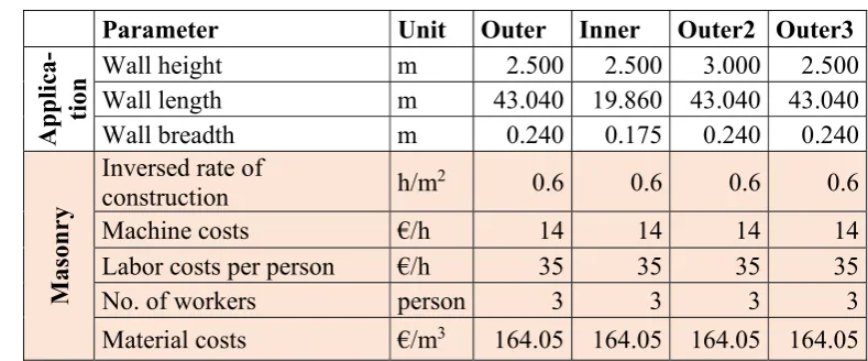
Table 1: Dimensions of the target application and corresponding calculated parameters for laboratory 456
buildability testing. 457
Parameter Unit Outer Inner Outer2 Outer3
Appli
ca-tion
Wall height m 2.500 2.500 3.000 2.500 Wall breadth m 0.240 0.175 0.240 0.240 Aspect ratio 10.417 14.286 12.500 10.417
Lab
Layer breadth m 0.030 0.030 0.030 0.060 Layer thickness m 0.020 0.020 0.020 0.020 Height to be tested m 0.313 0.429 0.375 0.625
No of layers # 16 21 19 31
The material explicitly considered in this article is a high-strength, fine-grained concrete M, its 458
compressive strength at an age of 28 days exceeding 80 MPa, developed for the outer load-bearing 459
walls of the target residential buildings. Thus, for the laboratory buildability tests, case ‘Outer’ 460
presented in Table 2 will be considered. Table 2 shows that to ascertain the buildability of the 461
mixture M, 16 layers have to printed in the laboratory, complying with maximum time-interval and 462
prescribed tolerances, for example, according to the German standard DIN 18202:2013-04 [26]). 463
The handling of the cases other than Outer should follow the same routine. 464
Figure 5: Sketch of a representative target residential building. 466
3.2 Time interval (TI)
467
The calculations presented below are valid for walls of one floor of a multi-story house erected 468
using CONPrint3D; for purposes of comparison an estimation for walls made of conventional 469
masonry are provided too. The process parameters of masonry construction are given in Table 2; 470
here the use of sand-lime bricks is assumed. These are used to calculate the construction costs for 471
the masonry work and to derive VDC,min.
472
Table 2: Dimensions of the target application and process parameters of example masonry constructions 473
Parameter Unit Outer Inner Outer2 Outer3
Appli
ca-ti
on
Wall height m 2.500 2.500 3.000 2.500 Wall length m 43.040 19.860 43.040 43.040 Wall breadth m 0.240 0.175 0.240 0.240
Masonry
Inversed rate of
construction h/m2 0.6 0.6 0.6 0.6
Machine costs €/h 14 14 14 14
Labor costs per person €/h 35 35 35 35
No. of workers person 3 3 3 3
Material costs €/m3 164.05 164.05 164.05 164.05
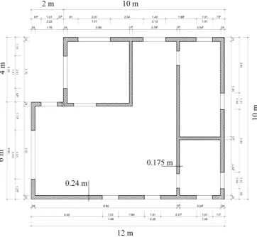
The outer wall length of 43.04 m and the inner wall length of 19.86 m as presented in Table 2 are 474
calculated from the floor layout of the target application, presented in Figure 6. To calculate the 475
printhead travel length for each layer to be deposited, it is essential to address “printing scenarios” 476
or the aspect of “tool-path optimization”. For the sake of simplicity, in the example presented here 477
we assume that one complete layer along the outer walls is printed first. Subsequently, further 478
layers of the outer walls are added upon one another. After the completion of the outer walls, the 479
inner walls are produced and frictionally connected to the outer walls by stainless steel anchors, 480
which are inserted into each layer. In contrast to this simple scenario, the path of the printhead can 481
be defined in numerous ways, as shown in Figure 7, while various algorithms can be utilized for 482
determining the optimum printing scenario. In such cases, the wall length in Table 3, must be 483
It is noteworthy that the choice of a suitable starting point and the minimization of idle-traverses
485
(travel times without concrete discharge, shown with the dashed line in Figure 7) are of great 486
importance in any printing strategy. 487
488
Figure 6: Layout and dimensions of a storey of the target house. 489
The optimal printing path depends on numerous boundary conditions. An essential optimization 490
criterion is the path length. While the shortest printing path should be generally preferred, it cannot 491
always be used due to other constraints, such as the motion and clearance profiles of the printhead 492
or on-site construction process conditions. Zhang et al. [36] adapted the so-called “traveling 493
salesman problem (TSP)” to determine the optimal tool path for constructing with Contour Crafting 494
technology. They derived the shortest paths by adding multiple vertices in the corners and wall 495
connections, and then by transforming the optimization problem from the node-oriented to the 496
498
499
Figure 7: Various scenarios for printing the walls of a house considered under consideration. 500
The rate at which masonry construction takes place is generally expressed in terms of the time 501
needed to complete a square meter of a wall, usually an hour. Since this rate is inverse to the rate 502
generally considered in concrete construction rates, i.e., unit area per unit time, more specifically 503
square meters per hour, it is termed here inversed rate of construction with a notation RI; see 504
Section 2. The RI values used in the articles at hand are according to 505
Baukosteninformationszentrum Deutscher Architektenkammern (BKI) for the masonry wall type 506
KS-L-R 8 DF 240 mm [37]. The rate of construction is given per person, thus, when deriving VDC
507
using Eq. 17, one must multiply RI with actual number of workers working on the masonry 508
application, which is in this case three, leading to an effective RI of 0.2 h/m2.
509
Machine costs presented in Table 4 for a small crane (Kleinkran C.2.00.0007I) are in accordance 510
with BGL 2015 [38]. These costs include repair, depreciation and interest costs. The material costs 511
are also calculated for the masonry wall type Format KS-L-R 8 DF 240 mm and include delivery 512
and mortar costs [37]. Process parameters of the CONPrint3D are presented in Table 4, which are 513
used to calculate the construction costs and derive VDC,min.
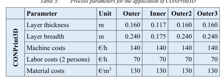
Page | 18 Table 3: Process parameters for the application of CONPrint3D
515
Parameter Unit Outer Inner Outer2 Outer3
CON
P
rint3
D Layer thickness m 0.160 0.117 0.160 0.160
Layer breadth m 0.240 0.175 0.240 0.240
Machine costs €/h 140 140 140 140
Labor costs (2 persons) €/h 70 70 70 70
Material costs €/m3 130 130 130 130
Since CONPrint3D is an FWP process, the breadth of the printed layer is equal to the breadth of 516
the target wall. For the case “Outer” considered here, the breadth of a printed layer is 0.24 m. The 517
thickness of the layer is a process parameter which affects the total number of layers to be printed, 518
total printing time, and hence construction costs. The maximum feasible layer thickness depends 519
on the material properties. For the case presented here, layer thickness was assumed to be two-520
thirds of the layer breadth in accordance with the geometrical proportions of the nozzle of the lab 521
printer. Numerous scaled-down wall-elements, including those in Figure 4, had been already 522
printed using the aforementioned nozzle-aspect ratio. Machine costs for CONPritn3D as given in 523
Table 4 are, at the current stage, higher than that of masonry construction. They include costs for a 524
modified concrete boom pump, costs for transporting concrete from mixing plant to construction 525
site and costs for adjusting and calibrating the pump on the site. In general, for DC technologies 526
lower manpower costs are envisioned in comparison to conventional construction. In the case of 527
CONPrint3D two workers would be necessary from today’s perspective: one for machine 528
monitoring and one for auxiliary works. Based on BKI 2017 values, the average wage of one 529
person is calculated at 35 € per hour [37]. 530
The material costs for CONPrint3D, 130.00 €/m3, are calculated conservatively for high-strength,
531
fine-grained concrete M used in experiments. They include material costs for admixtures and 532
additives (micro-silica suspension, fly ash and superplasticizer). In sum, the material costs are
533
approximately 70 % higher in comparison to the material costs for ordinary concrete of the strength
534
class C25/30 in conventional construction. The mixture M, containing expensive additives and
535
admixtures, was chosen deliberately for the calculations to ensure process-safe implementation of
536
the onsite digital construction of load-bearing elements since printable concrete is, in general, likely
537
to contain fine mineral additives and chemical admixtures to achieve the required rheological,
538
mechanical and/or durability characteristics. While for the target residential building application,
539
the required concrete class according to DIN EN 206-1 is C25/30. The fine-grained concrete 540
considered here has a compressive strength of 100 MPa at an age of 28 days. Thus, a considerable 541
reduction in material costs is feasible in the course of the optimization process. In addition to 542
material, machine and labor costs, 10 % additional costs are added to the total costs of CONPritn3D 543
as detailed in Section 2. 544
The minimum average printhead velocity Vdc,min for CONPritn3D application, to be equally
545
through 4. After knowing Vdc,min the maximum (again economically viable) TI between layers can 547
be calculated as TI = Lt / Vdc,min. Table 5 presents both Vdc,min and maximum TI calculated for various
548
cases of CONPrint3D application. For the Outer case, the time interval between extruding 549
subsequent layers should not exceed 51.61 minutes. In addition to the maximum TI it is also 550
possible to define the minimum TI based onthe maximum printing speed of the printer to be used. 551
Since the current laboratory printer for CONPrint3D has Vdc,max = 540.00 m/h, the minimum feasible 552
time interval can be calculated as TI = Lt / Vdc,max. The minimum TI for the Outer case is 4.78
553
minutes; see Table 5. It goes without saying that if printing of the entire construction were to occur 554
at a rate close to Vdc,max then the costs and construction time in case of CONPritn3D will be 555
considerably reduced in comparison to those of conventional construction. 556
Table 4: Process parameters of an example CONPrint3D application. 557
Parameter Unit Outer Inner Outer2 Outer3
Vdc,min m/h 50.04 72.04 50.04 100.08
Maximum TI min 51.61 16.54 51.61 51.61
Vdc,max m/h 540.00 540.00 540.00 540.00
Minimum TI min 4.78 2.21 4.78 4.78
3.3 Experimental validation
558
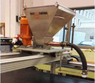
For production of the wall specimens, a custom-developed 3D-concrete-printing test device 559
(3DPTD) was used; see Figure 8. The 3DPTD is equipped with a progressive cavity pump to 560
extrude concrete. The speed at which a layer is printed and the time interval between the deposition 561
of two consequent layers can be pre-programmed. Details of the mechanical and electrical setup of 562
3DPTD are to be published elsewhere. The buildability of a fine-grained concrete M was validated 563
using the criteria proposed above. The composition of M can be found in [39]. The target 564
application considered is a residential house; see Section 3.1 and Figure 5. Specifically for the case 565
Outer see Tables 3 to 5. 566
567
Figure 8: Printhead of 3DPTD consisting of concrete hopper, progressive-cavity extruder and nozzle.
568
The design of the buildability experiment is to produce 𝑛 number of layers with TI minutes 569
of time interval between layers. If the printed wall retains its geometry and dimensions then the 570
tested material is applicable for the target application. As determined in Sections 3.1 and 3.2, a 571
mentioned here is the upper limit. TI longer than 61.24 minutes adversely affects economic viability 573
if all other parameters are assumed constant. At a concrete age of 20 minutes from water addition 574
printing experiments were started by printing layers at a constant velocity of 150 mm/s and time 575
intervals of 3 minutes. Figure 9 shows the wall immediately after completion of the printing. Since 576
16 layers could be printed with a TI much shorter than the economically required TI, the mixture 577
M could be designated “buildable” for the considered application case. 578
Figure 9: 16-layer wall specimen printed using fine-grained concrete M with time intervals of 3 minutes between
579
layers. 580
4. Buildability requirements for filament printing and full-width printing 581
Buildability requirements for a material depend not only upon the target structure but also on the 582
printing approach applied. The ‘height’ component of the buildability criteria remains essentially 583
the same for both the full-width printing (FWP) and filament printing (FP) approaches. In contrast, 584
the ‘effective length’ of each layer to be printed, i.e. total travel distance, often greater than the 585
length of the actual wall, varies significantly between FWP and FP, which directly affects TI as 586
well. If a single-nozzle opening is used, as in [2,4,5,10,40], in the case of FP, the printhead travels 587
approximately twice the distance in comparison to FWP to complete the deposition of the outer 588
filaments; see Figure 10. Furthermore, additional time is needed to place the inner wave-like 589
filament. Since in the case of full-width printing the entire layer cross-section is printed in one run, 590
printhead velocity Vprinthead,FWP, the velocity calculated using distance travelled by the printhead,
591
is equal to the “effective” horizontal velocity of printing Veffective,FWP, velocity being calculated
592
using displacement along the wall length. For FP, in contrast, even if printhead velocity Vprinthead,FP
593
is kept the same as Vprinthead,FWP, the “effective” horizontal velocity of construction Veffective,FPwill
594
be lower than Veffective,FWP. Consequently, to achieve an equal construction rate in the case of FP,
595
printhead velocity Vprinthead,FP has to be much higher than in the case of FWP. A simplistic
596
approximation for FP can be: 597
Vprinthead,FP = Veffective,FP (2+k) with k = f(λ,û) Eq. 20
where λ is the wavelength and û is the amplitude of the wave depicting the inner filament of the 599
wall produced by means of FP; see Figure 10c. 600
Since the Veffective of FP is much lower than that of FWP the TI between layers in case of FP is also
601
longer. Although it may appear advantageous in terms of “available” resting time for structural 602
build-up, a longer TI means a reduction in the economic viability and a higher risk of formation of 603
“cold joints”, weak interface strengths, between layers. Savings in material through FP in 604
comparison to FWP are less significant: as Tables 3 and 4 show, material costs are not the major 605
contributor for the total construction costs. 606
From a rheological perspective, Eq. 20 implies the following two cases summarized in Table 5, 607
where FP is compared to FWP for the same target application. 608
Table 5: Requirements in case of FP depending on the comparative constant. 609
Comparative cases of FP and FWP FP requires
1 Constant economic viability • Higher Vprinthead,FP
• Higher rates of material pumping and extruding, thus higher pumpability and extrudability.
• Lower plastic viscosity.
2 Constant printhead speed Vprinthead • Lower buildability (TI will be higher) • higher open-time/working-window of
the construction material
• Longer construction times
It is of interest mathematically to describe the above-mentioned intricacies of buildability 610
requirements for FP and FWP in order to facilitate: 611
• Choice between FP and FWP, if the choice of material is restricted; 612
• Extension of the model presented in Section 2 to FP cases by providing a mathematical 613
description of TI in terms of wall geometry, for instance, the minimum TI in the case of FP 614
be calculated using Eq. 30-32; 615
• Development of process-agnostic, printable concretes, i.e. concretes applicable for both FP 616
and FWP processes. 617
The following is the derivation for the needed Vprinthead,FP in relation to Vprinthead,FWP, provided only
618
one nozzle is used and constant economic viability or constant construction rate is to be achieved 619
(Case 1 in Table 5). 620
Page | 22 Assuming
622
• length of the wall to be produced: L, 623
• distances that the printhead travels in case of FWP (Figure 10a): L1,
624
• distances that printhead travels in case of FP (Figure 10b, -c): L2 for outer and L3 for inner 625
profile, 626
we obtain: 627
time for printhead travel in FWP: tFWP = L1/Vprinthead,FWP = L1/Veffective,FWP and
628
time for printhead travel in FP: tFP = (L2+L2+L3)/Vprinthead,FP.
629
Assuming equal economic viability in FP and FWP as in Case 1 (Table 5), both the times should 630
be equal, thus: 631
, = , Eq. 21
632
𝑉 , = 𝑉 , Eq. 22
633
634
635
636
Figure 10: Schematic views of the top sectional views of two walls of identical length and width, produced through
637
a) full-width-printing FWP) and b) filament-printing FP. The FP figure also illustrates two additioanl alternatives 638
-0.075 -0.025 0.025 0.075
0 0.5 1 1.5 2 2.5 3 3.5 4
Breadt
h
ß
[m
]
Length of wall L [m]
-0.075 -0.025 0.025 0.075
0 0.5 1 1.5 2 2.5 3 3.5 4
Breadt
h ß
[m
]
Length of wall L [m]
λ = 0.3 λ = 0.6 λ = 1
ß b
λ
f(x)=(ß/2-b)sin(2Пx/λ)
Length = L=L1=L2 Length = L3 > L a)
b)
for inner filament defined by wavelengths λ. c) A scheme showing wavelength and semi-amplitude of sinusoid 639
dipcting inner filament in FP. 640
Since the length of the wall L = L1 = L2 ≠ L3 Eq. 23 641
𝑉 , = 2 + 𝑉 , Eq. 24
642
Expressing the inner filament in FP as a sinusoid 𝑦 = 𝑖 sin 𝑗 𝑥 from 0 to L
643
Length (distance between 0 and L) of the inner filament is 644
L3 = 1 + ((𝑖 ∗ 𝑗) 𝑐𝑜𝑠 𝑗 𝑥 dx Eq. 25
645
With i = semi-amplitude of the inner filament = Û = ß/2-b
646
and j = 2П/ λ
647
where ß and b are the breadth of the produced wall and filament, respectively, and λ is the 648
wavelength of the inner filament; see Figure 10c. 649
Length of the inner filament expressed in sinusoid attributes can be calculated according to Eq. 650
26: 651
L3= 1 + ((ß− 𝑏) ∗ ) 𝑐𝑜𝑠 dx Eq. 26
652
From Eq. 17 and Eq. 19 we obtain: 653
𝑉 , = 2 +
((ß )∗ )
𝑉 , Eq. 27
654
Equation 27 enables determination of printhead velocity to be followed while applying FP to retain 655
economic viability equal to that of FWP processes. 656
Still further, if equal economic viability is not the primary concern and constant printhead speed is 657
followed for both FP and FWP, i.e. Case 2 in Table 5, then a higher minimum TI is valid for FP. 658
The following relationship between TImin,FP and TIminFWP can be obtained:
659
𝑇𝐼 , = 𝑇𝐼 , Eq. 28
660
𝑇𝐼 , = 2 +
((ß )∗ )
𝑇𝐼 , Eq. 29
661
In addition, with no comparison to FWP, the minimum TI in case of FP can be calculated for a 662
printhead velocity of Vprinthaed:
663
𝑇𝐼 , =
((ß )∗ )
Eq. 30
664
Eq. 30 is a generalized formula to determine the minimum time intervals between layers, which 665
formula must be followed during laboratory buildability tests if an element of target length L is 666
produced through FP. 667
It must be noted that Eq. 30 is valid only if one nozzle is used to print the filaments; see Figure 668
a) Two passes are needed for one horizontal layer of the target wall. In the first pass, two 670
nozzles extrude the outer ‘shells’ and in the second pass, one nozzle extrudes the inner 671
‘wave’; see Figure 11b. An example of this scenario is demonstrated by Contour Crafting 672
[41]. 673
b) One pass is needed for one horizontal layer of target wall. Two nozzles extrude the outer 674
‘shells’ and in parallel, a third nozzle prints the inner ‘wave’. To the best of authors’ 675
knowledge, this scenario has not yet been demonstrated. 676
Moreover, in both scenarios one additional pass of the printhead or other devise will be needed if 677
spaces between ‘shells’ and ‘wave’ need to be filled, e.g. with insulating materials or (self-678
compacting) concrete; see Figure 11c. 679
For the scenarios ‘a’ and ‘b’ mentioned above, Eq. 30 can be transformed to Eq. 31 and Eq. 32, 680
respectively: 681
V , = 1 +
((ß )∗ )
V , Eq. 31
682
V , =
((ß )∗ )
V , Eq. 32
683
Similarly, Eq. 29 and Eq. 30 can be reformulated according to the number of nozzles used. As can 684
be seen in Eq. 32, even if three nozzles are used and moved at the same speed as in case of FWP, 685
the effective printing velocity in case of FP will be lower in comparison to FWP due to the longer 686
absolute traveling length. 687
688
Figure 11: Various scenarios for printing “one set of horizontal layers” in case of FP printing process: a) single
689
nozzle – three passes are needed [42], b) three nozzles – two passes are needed [41] and c) representation of single 690
nozzle with “post-filling” of the empty space between layers [43]. 691
Based on the deduced relationships, it can be concluded that when testing the buildability of a 692
material for FP processes, generally higher velocities of the printhead are to be followed during 693
laboratory tests in comparison to corresponding tests for FWP. 694
695
![Figure 1. Examples of digital construction approaches: a) structural elements produced on-site using selective material deposition by extrusion [4], b) complex structure of Digital Grotesque II produced in a stationary 3D-printer using selective binding technique [11]](https://thumb-us.123doks.com/thumbv2/123dok_us/1085065.1609169/2.595.71.526.516.659/examples-construction-approaches-structural-deposition-structure-grotesque-stationary.webp)
![Figure 2. a) CONPrint3D technology as example of full-width printing [courtesy: Chair of Construction Machines, TU Dresden], b) Contour Crafting as example of filament printing [courtesy: Contour Crafting], c) Wonder Bench at Loughborough University as ex](https://thumb-us.123doks.com/thumbv2/123dok_us/1085065.1609169/3.595.69.529.177.379/conprint-technology-construction-machines-crafting-crafting-loughborough-university.webp)