Discrete Sine Transform-Based Interpolation Filter for Video Compression

Article

1

Discrete Sine Transform-Based Interpolation Filter

2

for Video Compression

3

MyungJun Kim and Yung-Lyul Lee *

4

Department of Computer Engineering, Sejong University, Seoul 05006, Korea; [email protected]

5

* Correspondence: [email protected]

6

Abstract: High Efficiency Video Coding (HEVC) uses an 8-point filter and a 7-point filter, which

7

are based on the discrete cosine transform (DCT), for the 1/2-pixel and 1/4-pixel interpolations,

8

respectively. In this paper, discrete sine transform (DST)-based interpolation filters (IF) are

9

proposed. The first proposed DST-based IFs (DST-IFs) use 8-point and 7-point filters for the

10

1/2-pixel and 1/4-pixel interpolations, respectively. The final proposed DST-IFs use 12-point and

11

11-point filters for the 1/2-pixel and 1/4-pixel interpolations, respectively. These DST-IF methods

12

are proposed to improve the motion-compensated prediction in HEVC. The 8-point and 7-point

13

DST-IF methods showed average BD-rate reductions of 0.7% and 0.3% in the random access (RA)

14

and low delay B (LDB) configurations, respectively. The 12-point and 11-point DST-IF methods

15

showed average BD-rate reductions of 1.4% and 1.2% in the RA and LDB configurations for the

16

Luma component, respectively.

17

Keywords: HEVC; Interpolation filter; Sinc; DCT (discrete cosine transform); DST (discrete sine

18

transform)

19

1. Introduction

20

The ITU Telecommunication Standardization Sector-Video Coding Expert Group (ITU-T

21

VCEG) and the Moving Picture Expert Group (ISO/IEC MPEG) organized the Joint Collaborative

22

Team on Video Coding (JCT-VC) [1], and they jointly developed the next-generation video-coding

23

standard HEVC/H.265. In HEVC [2], motion-compensated prediction (MCP) is a significant

24

video-coding function that reduces the temporal redundancy in video signals. In the MCP, each

25

prediction unit (PU, block) in the encoder finds the block that has the least SAD (sum of absolute

26

difference) from the reference pictures in terms of the Lagrangian cost [3]. Since the moving objects

27

between two pictures are continuous, it is difficult to identify the actual motion vector in

28

block-based motion estimation. Therefore, the use of fractional pixels that have been derived from

29

an interpolation filter for motion-vector searches can improve the precision of the MCP.

30

The sinc function is an ideal interpolation filter in terms of signal processing [4], [5]. However,

31

the sinc-interpolation filter is difficult to implement in HEVC because the sinc-interpolation filter

32

needs to reference the neighbor pixels from -∞ to ∞. Therefore, the HEVC interpolation filters are

33

designed from the DCT type-II (DCT-II) transform [6], [7], [8] that improves the bit reduction by

34

approximately 4.0 % compared with the H.264/AVC interpolation filters [9]. The filter lengths of the

35

DCT-II-based interpolation filter (DCT-IF) are 8-point and 7-point for the 1/2-pixel and 1/4-pixel

36

interpolations, respectively. In the present paper, a DST [10]-based interpolation filters (DST-IFs)

37

that use different interpolation-filter lengths are proposed.

38

This paper is organized as follows. Section 2 presents the ideal interpolation filter, the sinc

39

function, the DCT-IF, the proposed DST-IF, and an analysis of the interpolation filters. Section 3

40

presents the experiment results, and Section 4 concludes the paper.

41

42

43

44

2. Interpolation Filters for Generating Fractional Pixels

45

2.1 The sinc-based interpolation filter

46

The sinc-based interpolation filter is an ideal interpolation filter in terms of signal processing

47

and its equation is as follows:

48

sin ( )

( ) ( ) ( ) s s s k s s t kT T x t x kT

t kT T π π ∞ =−∞ − = −



where the sinc-based interpolation filter is defined as x(t), t represents the locations of the

49

subsamples and k is the integer sample value, and Ts is the sampling period that is equal to 1. When

50

the sinc-based interpolation filter is lengthened from -∞ to ∞, it is the ideal interpolation filter to

51

reconstruct all the samples. Although the sinc-based interpolation filter is ideal, it is not possible to

52

implement it in HEVC. Since it is impossible to reference all of the neighbor pixels in a picture, the

53

DCT-IF is adopted in HEVC, the filter lengths of which are restricted within 8-point and 7-point for

54

the 1/2-pixel and 1/4-pixel interpolations, respectively.

55

2.2 The DCT-II interpolation filter (DCT-IF) in HEVC

56

The DCT-IF [4] in HEVC is designed in a different way but it can be designed easily in this

57

paper from the following forward/inverse DCT-II:

58

1 0

2 ( 1/ 2)

( ) Nn k ( ) cos

n k

X k c x n

N N

π

− =

+

=



1 0

2 ( 1/ 2)

( ) kN k ( ) cos

n k

x n c X k

N N

π

− =

+

=



In Equation (1), X(k) is the DCT-II coefficients and the input pixel x(n) is the IDCT-II (Inverse

59

DCT-II) coefficients in Equation (2).

60

61

1 _{, k=0} 2 1 , otherwise k c   =  (3)

62

where ck is 1/√2 at k=0, and ck is 1 at k≠0. The substitution of Equation (1) into Equation (2) results in

63

the following DCT-IF equation:

64

65

1 _{1 2}

0 0

2 ( 1/ 2) ( 1/ 2)

( ) _mN ( ) _kN kcos cos

m k n k

x n x m c

N N N

π π

− −

= =

+ +

=





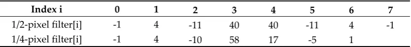
Table 1. 8-point and 7 point DCT-II based Interpolation Filter Coefficients in HEVC.

Index i 0 1 2 3 4 5 6 7

1/2-pixel filter[i] -1 4 -11 40 40 -11 4 -1

1/4-pixel filter[i] -1 4 -10 58 17 -5 1

66

For example, the 1/2-pixel interpolation filter, when n = 3.5, in the 8-point DCT (N = 8) is derived

67

as a linear combination of the cosine coefficients and x(m), m = 0,1,…,7. Similarly, the 1/4-pixel

68

cosine coefficients and x(m), m = 0,1,…,6. Lastly, the DCT-IFs that interpolate the 1/2-pixel and

70

1/4-pixel interpolations are shown as the integer numbers in Table 1. The filter-coefficient order of

71

the 3/4-pixel interpolation filter is the reverse of the filter-coefficient order of the 1/4-pixel

72

interpolation filter.

73

74

75

Figure 1. Fractional pixel position in Luma motion compensation.

76

Figure. 1 is an example of the integer- and fractional-pixel positions in the Luma motion

77

compensation. In Figure 1, the capital letters (A0 to A7) indicate the integer-pixel position, the small

78

letter b0 is the 1/2-pixel position, and a0 and c0 are the 1/4-pixel and 3/4-pixel positions, respectively.

79

For example, using the DCT-IF, the b0 and a0 are calculated from Table 1 as follows:

80

0

( 1

4

11

40

40

11

4

1

32)

6

b

= − ⋅ + ⋅ − ⋅ + ⋅ + ⋅ − ⋅ + ⋅ − ⋅ +

A

A

A

A

A

A

A

A



0

( 1

4

10

58

17

5

1

32)

6

a

= − ⋅ + ⋅ − ⋅ + ⋅ + ⋅ − ⋅ + ⋅ +

A

A

A

A

A

A

A



(5)

where the computation of a0 is the same as that of b0 from Table 1, the computation of c0 is in the

81

order that is the reverse of that of a0, and “>>” operation means the bit-wise shift right.

82

2.3 The Proposed DST-VII Interpolation Filter (DST-IF)

83

The DST-IF for HEVC can easily be designed in this paper from the forward/inverse DST-VII.

84

The DST-VII and inverse DST-VII are defined as follows:

85

1 0

1

( 1)( )

2 ₂

( ) ( )sin

1 1

2 2

N n

n k

X k x n

N N π − = + + = +



( 1)( )

2 ₂

( ) ( )sin

1 1

2 2

N k

n k

x n X k

N N π − = + + =

+



where X(k) is the DST-VII coefficient and x(n) represents the input pixels. The substitution of

86

Equation (6) into Equation (7) results in the following DST-IF equation:

87

1 1

0 0

1 1

( 1)( ) ( 1)( )

2 _{2 2}

( ) ( ) sin sin

1 1 1

2 2 2

N N

m k

m k n k

x n x m

N N N

π π

− −

= =

+ + + +

=

+





In the similar way to obtain the DCT-IF coefficients, the DST-IF is derived from Equation (8).

88

For example, the 1/2-pixel interpolation filter, when n = 3.5, in the 8-point DST (N = 8) is derived as a

89

linear combination of the sine coefficients and x(m), m = 0,1,…,7. Similarly, the 1/4-pixel

90

interpolation filter, when n = 3.25, in the 7-point DST (N = 7) is derived as a linear combination of the

91

sine coefficients and x(m), m = 0,1,…,6. Lastly, the DST-IFs that interpolate the 1/2-pixel and

92

1/4-pixel interpolations are shown in Table 2. The filter-coefficient order of the 3/4-pixel

93

interpolation filter is the reverse of the filter-coefficient order of the 1/4-pixel interpolation filter [11].

94

Table 2. 8-point and 7 point DST-VII-based Interpolation-Filter (DST-IF) Coefficients.

95

Index i 0 1 2 3 4 5 6 7

1/2-pixel filter[i] -2 6 -13 41 41 -13 6 -2

1/4-pixel filter[i] -2 5 -11 58 18 -6 2

96

In the given example, the 8-point and 7-point DST-IFs were derived, but the M-point and

97

(M-1)-point DST-IFs, where M > 8, can be easily derived in a similar way for high-resolution

98

Table 3. 12-point and 11-point DST-VII-based Interpolation-Filter (DST-IF) Coefficients.

100

Index i 0 1 2 3 4 5 6 7 8 9 10 11

1/2-pixel filter[i] -1 2 -4 7 -13 41 41 -13 7 -4 2 -1

1/4-pixel filter[i] -1 2 -3 6 -11 58 19 -8 4 -3 1

Table 4. 12-point and 11-point DCT-II-based Interpolation-Filter (DCT-IF) Coefficients.

101

Index i 0 1 2 3 4 5 6 7 8 9 10 11

1/2-pixel filter[i] -1 2 -4 7 -12 40 40 -12 7 -4 2 -1

1/4-pixel filter[i] -1 2 -3 5 -11 58 18 -7 4 -2 1

102

The 12-point and 11-point DST-IFs that interpolate the 1/2-pixel and 1/4-pixel interpolations are

103

shown in Table 3. The 12-point and 11-point DST-IFs in Table 3 are derived in this paper from

104

Equation (8), where N = 12 and n = 5.5 and N = 11 and n = 5.25, respectively. In the similar way, the

105

12-point and 11-point DCT-IFs in Table 4 are derived in this paper.

106

2.4 Analysis of the interpolation filters

107

108

Figure 2.Magnitude Responses of Interpolation Filters for the 1/2-pixel Position in the Luma Component.

109

110

Figure 2 shows all of the different graphs of the magnitude responses of the 1/2-pixel

111

interpolation filters. In the x-axis, the discrete time frequency

ω

ˆ

112

1, where 1 corresponds to the π radian. The y-axis is the magnitude response. Figure 2 illustrates the

113

magnitude-response graphs of five (5) interpolation filters reconstructing the 1/2-pixel position. The

114

sinc function, which is assumed the ideal interpolation filter, is designed with a 48-point

115

interpolation filter and represented by a dot-line. The 48-point sinc interpolation filter has relatively

116

high frequency response even around

ω

ˆ

117

8-point DCT-IF, 8-point DST-IF, 12-point DCT-IF, and 12-point DST-IF and it comprises many more

118

ripples at high frequencies compared with the other interpolation filters. In particular, in the low

119

frequency responses when

ω

ˆ

120

interpreted that all five (5) interpolation filters have similar low frequency responses but the high

121

frequency responses are different. Comparing the 8-point DCT-IF drawn in a gray line and the

122

8-point DST-IF drawn in a black line, the 8-point DST-IF has relatively high frequency responses

123

similar. In case of the 12-point DST-IF and 12-point DCT-IF, which are represented by a green and

125

red line, two interpolation filters have relatively higher frequency responses than the 8-point

126

DST-IF and 8-point DCT-IF even if the low frequency responses are quite similar. The 12-point

127

DST-IF and the 12-point DCT-IF have similar high frequency responses because they have almost

128

similar interpolation filter coefficients as shown in Table 3 and Table 4 where only the filter

129

coefficients of integer pixel position 4,5,6,7 are different in 1/2-pixel filter coefficients. It means that

130

12-point DST-IF and 12-point DCT-IF are similar when they are derived mathematically. Therefore,

131

comparing the 12-point DST-IF with 8-point DCT-IF and DST-IF and 12-point DCT-IF in Figure 2,

132

the 12-point DST-IF shows relatively high frequency responses, even though the 48-point sinc

133

interpolation filter shows better high frequency responses than other four (4) interpolation filters.

134

135

3. Experimental Results

136

3.1. Experimental Conditions

137

The proposed DST-IF was implemented in the HEVC reference software, HM-16.6 [12],

138

according to the HEVC common-test conditions. Table 5 shows the test sequences where the

139

sequences of the classes B, C, D, and E comprise the resolutions of 1080p, 832 × 480, 416 × 240, and

140

720p, respectively, and the proposed method was applied when the quantization-parameter (QP)

141

values were 22, 27, 32, and 37, respectively. Table 6 and Table 7 show the test sequences and the

142

BD-rate gain compared with those of HM-16.6 for the Luma component in the LDB, low delay P

143

(LDP), and RA configurations, respectively. The random access configuration has hierarchical B

144

pictures (IBBBBBBBP) which have a GOP (Group of pictures) size of eight (8). The low delay

145

structure is composed of the first I (intra) picture and following P (Predictive) pictures (IPPPPP…).

146

The P pictures in the low delay structure are GPB’s (Generalized P and B pictures), in which the P

147

pictures are replaced by B pictures having the same two reference pictures.

148

The negative sign of the BD-rate represents the bit-saving of the proposed method compared

149

with that of HM-16.6 in the same PSNR (peak signal-to-noise ratio) reference [13].

150

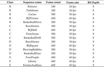
Table 5. Test Sequences used in HEVC Common-Test Conditions.

151

Class Sequence name Frame count Frame rate Bit Depth

B Kimono 240 24 fps 8

B ParkScene 240 24 fps 8

B Cactus 500 50 fps 8

B BQTerrace 600 60 fps 8

B BasketballDrive 500 50 fps 8

C RaceHorses 300 30 fps 8

C BQMall 600 60 fps 8

C PartyScene 500 50 fps 8

C BasketballDrill 500 50 fps 8

D RaceHorses 300 30 fps 8

D BQSquare 600 60 fps 8

D BlowingBubbles 500 50 fps 8

D BasketballPass 500 50 fps 8

E FourPeople 600 60 fps 8

E Johnny 600 60 fps 8

E KristenAndSara 600 60 fps 8

3.2. Experimental Results

153

Table 6. DST-IF Bit-saving Results applied to Uni- and Bi-directional Prediction.

154

Saving Bits(%)

8-point and 7-point DST-IF

12-point and 11-point DST-IF / 12-point and 11-point

DCT-IF

Class Sequence name LDB LDP RA LDB LDP RA

B Kimono 0.3 1.2 0.2 0.6/0.5 2.5/0.5 0.2/0.3

B ParkScene 0.8 2.1 0.3 1.7/1.3 3.9/1.6 0.5/0.9

B Cactus 0.8 2.3 0.2 1.1/1.2 3.6/1.6 0.0/0.8

B BasketballDrive 0.1 1.2 0.1 0.3/0.4 2.3/0.6 0.3/0.3

B BQTerrace 1.5 5.3 1.0 2.7/3.4 8.6/4.4 1.5/2.3

C RaceHorses -0.9 0.3 -0.2 -1.2/-0.7 0.6/-0.1 -0.5/-0.2

C BQMall -0.2 1.3 -0.5 -0.5/-0.6 1.8/-0.2 -1.0/-0.5

C PartyScene -1.7 -0.2 -2.5 -3.5/-4.4 -1.7/-3.6 -4.5/-3.8

C BasketballDrill 0.6 1.7 0.4 1.2/0.9 2.9/1.1 0.8/0.6

D RaceHorses 0.1 0.8 -0.1 0.0/-0.2 1.2/0.0 -0.3/-0.2

D BQSquare -4.1 -0.4 -5.2 -7.5/-7.2 -2.9/-4.9 -9.0/-7.4

D BlowingBubbles -1.5 0.0 -1.8 -2.8/-3.1 -0.9/-2.2 -3.1/-2.4

D BasketballPass 0.5 1.2 0.2 0.9/0.9 2.0/1.1 0.4/0.4

E FourPeople 0.6 2.4 x 1.2/1.2 4.7/1.6 x

E Johnny 0.5 4.4 x 1.0/1.9 9.0/2.3 x

E KristenAndSara 0.6 2.4 x 1.2/1.5 5.5/1.4 x

Overall -0.1 1.6 -0.6 -0.2/-0.2 2.7/0.3 -1.1/-0.7

155

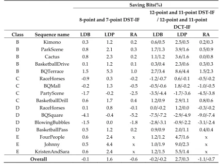
HM-16.6 uses an 8-point filter and a 7-point filter for the 1/2-pixel and 1/4-pixel interpolations,

156

respectively. From Table 6, the average bit-saving (BD-rate gain) in the RA configuration was

157

improved by 0.6 % with the use of the 8-point DST-IF for 1/2-pixel and 7-point DST-IF for 1/4-pixel.

158

Especially, the result of BQSquare in Class D achieved a bit-saving up to 5.2 % in the RA

159

configuration. The average bit-savings of 0.6 % and 0.1 % were achieved in the RA and LDB

160

configurations, respectively. However, the average bit-saving was decreased by 1.6 % in the LDP

161

configuration. In Table 6, the 12-point and 11-point DST-IFs that were applied to HM-16.6 also

162

showed bit-saving in the RA and LDB configurations and bit-increasing (BD-rate loss) in the LDP

163

configuration. In Table 6, Class E sequences in the RA configuration are not experimented because

164

they are not experimental condition in the HEVC test. Those sequences are marked as x.

165

Interestingly, the DST-IFs in the LDP configuration show bit increments (BD-rate loss), while

166

the DST-IFs in the RA and LDB configurations show bit-savings. It’s because the backward

167

(uni-directional) prediction using the decoded past pictures provides the incomplete

168

motion-compensated block compared with the bi-directional prediction that utilizes the average

169

pixel values of two different blocks that were derived by the forward and backward

170

motion-compensations for subsample interpolation. Therefore, the proposed 12-point and 11-point

171

DST-IFs are applied only on the bi-directional motion-compensated blocks. The 12-point and

172

11-point DST-IFs, which are almost the same filter coefficients as the 12-point and 11-point DCT-IFs,

173

are effective on the bi-directional prediction. Table 7 shows the results of the DST-IF bit-saving

174

results applied only on the bi-directional prediction. In the RA and LDB configurations, the 8-point

175

and 7-point DST-IFs achieved bit-savings of 0.7 % and 0.3 % compared with HM-16.6, respectively,

176

HM-16.6, respectively. Table 7 shows the results of the 12-point and 11-point DCT-IFs as well. It

178

shows bit-savings of 0.6% and 0.7% in the LDB and RA configurations compared with HM-16.6,

179

respectively.

180

Table 7. DST-IF Bit-saving Results applied to Bi-directional Prediction.

181

Saving Bits(%)

8-point and 7-point DST-IF

12-point and 11-point DST-IF / 12-point and 11-point

DCT-IF

Class Sequence name LDB RA LDB RA

B Kimono 0.1 0.1 0.1/0.1 0.0/0.2

B ParkScene 0.2 0.1 0.0/0.3 0.0/0.6

B Cactus 0.2 0.0 -0.4/0.2 -0.3/0.6

B BasketballDrive 0.0 0.0 -0.1/0.1 -0.1/0.2

B BQTerrace 1.1 0.8 0.4/2.3 0.8/2.0

C RaceHorses -0.7 -0.2 -1.3/-0.5 -0.6/-0.2

C BQMall -0.3 -0.6 -1.2/-0.9 -1.3/-0.5

C PartyScene -1.5 -2.4 -3.8/-3.7 -4.4-3.5

C BasketballDrill 0.2 0.2 0.3/0.2 0.2/0.3

D RaceHorses -0.1 -0.2 -0.3/-0.2 -0.5/-0.2

D BQSquare -3.7 -5.0 -8.3/-6.3 -9.1/-6.9

D BlowingBubbles -1.2 -1.7 -2.9/-2.4 -3.0/-2.1

D BasketballPass 0.0 -0.1 -0.1/0.1 -0.1/0.2

E FourPeople 0.4 x -0.1/0.6 x/

E Johnny -0.4 x -1.5/0.2 x

E KristenAndSara 0.2 x -0.2/0.5 x

Overall -0.3 -0.7 -1.2/-0.6 -1.4/-0.7

182

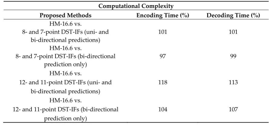
Table 8. Results of the Computational Complexity of the Proposed Method in the Low Delay B (LDB)

183

Configuration.

184

Computational Complexity

Proposed Methods Encoding Time (%) Decoding Time (%) HM-16.6 vs.

8- and 7-point DST-IFs (uni- and bi-directional predictions)

101 101

HM-16.6 vs.

8- and 7-point DST-IFs (bi-directional prediction only)

97 99

HM-16.6 vs.

12- and 11-point DST-IFs (uni- and bi-directional predictions)

118 113

HM-16.6 vs.

12- and 11-point DST-IFs (bi-directional prediction only)

104 107

Table 8 shows the computational-complexity results. As the 12-point and 11-point DST-IFs

186

reference four additional neighbor pixels compared with the 8-point and 7-point DST-IFs in HEVC,

187

when both the uni-directional and bi-directional predictions were applied, the computational

188

complexities in the encoding process and the decoding process were increased by 118 % and 113 %,

189

respectively. However, the 12-point and 11-point DST-IFs, which were applied on only the

190

bi-directional prediction, increased the computational complexity in the encoding process by 104 %

191

and in the decoding process by 107%. The computational-complexity of the 12-point and 11-point

192

DCT-IFs is almost same as that of the 12-point and 11-point DST-IFs. Even if the complexity of the

193

proposed 12-point and 11-point DST-IFs is increased compared with that of the existing 8-point and

194

7-point DCT-IFs in HEVC, the proposed method gives better bit-saving results than the existing

195

method.

196

For an alternative method, one interpolation filter was chosen between the DCT-IF and the

197

DST-IF, and this experiment has been tested using the coding unit-level rate-distortion optimization

198

[14], but the results are worse than those of Table 6 and Table 7 because one signaling bit is needed

199

to indicate which interpolation filter is used in the decoder side.

200

5. Conclusions

201

In this paper, DST-IF pairs of 12-point and 11-point filter lengths are proposed to achieve a

202

bit-rate reduction compared with the 8-point and 7-point DCT-IFs. Interestingly, the 12-point

203

DST-IF and the 12-point DCT-IF have similar high frequency responses because the 12-point DST-IF

204

and 12-point DCT-IF derived have almost similar interpolation filter coefficients as shown in Table

205

3 and Table 4. The experiment results show that the proposed DST-IF pairs achieved coding gains in

206

the RA and LDB configurations. However, as the bit-rate was increased in the LDP configuration

207

using the uni-directional prediction, the proposed DST-IF method was applied only on the

208

bi-directional prediction. Overall, the proposed 12-point and 11-point DST-IFs achieved average

209

BD-rate reductions of 1.4 % and 1.2 % compared with the 8-point and 7-point DCT-IFs in the RA and

210

LDB configurations of the Luma component, respectively. We believe this method can be

211

considered in the next video coding standard.

212

213

Acknowledgments: This research was in part supported by the National Research Foundation of Korea (NRF)

214

grant funded by the Korea government (Ministry of Science, ICT and Future Planning)

215

(NRF-2015R1A2A2A01006085)

216

Author Contributions: MyungJun Kim and Yung-Lyul Lee conceived and designed the experiments;

217

MyungJun Kim performed the experiments; Yung-Lyul Lee wrote the paper.

218

Conflicts of Interest: The authors declare no conflicts of interest.

219

References

220

1. B. Bros, W.-J. Han, J.-R. Ohm, G. J. Sulivan, Y.-K. Wang, and T. Wiegand, “High Efficiency Video Coding

221

(HEVC) text specification draft 10 (for FDIS & Consent),” document JCT-VC-L103, Jan. 2013.

222

2. Gary J. Sullivan, Jens-Rainer Ohm, Woo-Jin Han, and T. Wiegand, “Overview of the High Efficiency Video

223

Coding (HEVC) Standard,” IEEE Transactions on Circuits and Systems, no. 12, Dec. 2012.

224

3. C. Rosewarne, B. Bross, M. Naccari, K. Sharman, and Gary. J. Sullivan, High Efficiency Video Coding

225

(HEVC) Test Model 16 (HM 16) Improved Encoder Description Update 2, ITU-T/ISO/IEC Joint

226

Collaborative Team on Video Coding (JCT-VC) document JCTVC-T1002, Feb. 2015.

227

4. McClellan, James H., Ronald W. Schafer, and M. A. Yoder, “Signal Processing First,” Upper Saddle River,

228

NJ: Pearson/Prentice Hall, 2003.

229

5. Simon Haykin and Barry Van Veen, “Signals and Systems,” 2nd edition, Wiley 2003.

230

6. Kemal Ugur, Alexander Alshin, Elena Alshina, Frank Bossen, Woo-Jin Han, Jeong-Hoon Park, and Jani

231

Lainema, "Motion Compensated Prediction and Interpolation Filter Design in H.265/HEVC", IEEE in

232

7. Mathias Wien (2015). “High Efficiency Video Coding - Coding Tools and Specification,” Springer, Berlin

234

Heidelberg.

235

8. Vivienne Sze, Madhukar Budagavi, and Gary J. Sullivan (2014). “High Efficiency Video Coding (HEVC) –

236

Algorithms and Architectures,” Springer, Switzerland.

237

9. T. Wiegand, Gary J. Sullivan, G. Bjøntegaard, A. Luthra, “Overview of the H.264/AVC video coding

238

standard,” IEEE Transactions on Circuits and Systems, vol. 13, no. 7, pp. 560-576, Jul. 2003.

239

10. Stitch (2013), “Dicrete Sine Transform,” http://planetmath.org/sites/default/files/texpdf/39764.pdf

240

(accessed Sept, 2016).

241

11. MyungJun Kim, Nam-Uk Kim, Yung-Lyul Lee, “Investigation on interpolation filters in HEVC,” IWAIT

242

2017, January, 2017.

243

12. F. Bossen, “Common HM test conditions and software reference configurations,” Document of Joint

244

Collaborative Team on Video Coding, JCTVC-H1100, Feb. 2012.

245

13. G. Bjøntegaard, “Calculation of Average PSNR Differences between RD-curves”, ITU-T VCEG Meeting,

246

Austin, TX, USA, Tech. Rep. SG16 Q.6 Doc., VCEG-M33, Apr. 2001.

247

14. Gary. J. Sullivan, and T. Wiegand, “Rate-Distortion Optimization for Video Compression”, IEEE Signal

248