Article
Two-Dimensional Numerical Simulation Study on
Bed-load Transport in Fluctuating Backwater Area: A
Case-Study Reservoir in China
Ming Luo, Heli Yu, Er Huang *, Rui Ding and Xin Lu
State Key Lab. of Hydraulics and Mountain River Engineering,
College of Water Resource and Hydropower, Sichuan University, Chengdu 610065, China; [email protected] (M.L.); [email protected] (H.Y.); [email protected] (R.D.); [email protected] (X.L.) * Correspondence: [email protected]; Tel.: +86-151-981-63532
Abstract: Numerical modeling of sedimentation and erosion in reservoirs is an active field of reservoir research. However, simulation of bed-load transport phenomena has rarely been applied to other water bodies, in particular, the fluctuating backwater area. This is because the complex morphological processes between hydrodynamics and sediment transport are generally challenging to accurately predict. In this study, the refinement and application of a two-dimensional shallow-water and bed-load transport model to the fluctuating backshallow-water area is described. The model employs the finite volume method of the Godunov scheme and saturated sediment transport equations. The model was verified against experimental data of a scaled physical model. It was then applied to actual reservoir operation, including reservoir storage, reservoir drawdown and continuous flood process, to predict the morphology of reservoir sedimentation and sediment transport rates and bed level changes in the fluctuating backwater area. It was found that the location and morphology of sedimentation effected by the downstream water level results in random evolution of the river bed, and bed-load sedimentation is transported from upstream to downstream with the slope of the longitudinal section of the river bed generally reduced. Moreover, the sediment is mainly deposited in the main channel and the elevation difference between the riverbank and channel decreases gradually.
Keywords: fluctuating backwater area; reservoir; 2D shallow water equations; bed-load transport; Godunov-type scheme; FVM; non-uniformity sediment.
1. Introduction
The building of dams on rivers inevitably results in a disruption of the relative balance between river water and sediment condition. By trapping sediment in reservoirs, dams interrupt the continuity of sediment transport through rivers, resulting in loss of reservoir storage and reduced usable life, and depriving downstream reaches of sediment essential for channel form and aquatic habitats. With the acceleration of new dam construction globally, these impacts are increasingly widespread [1]. The erosion and sedimentation in the fluctuating backwater area of the reservoir is an important aspect of studying reservoir sedimentation, which have a considerable effect on the sedimentation of the entire reservoir and increase of backwater elevation. These processes in particular play an important role in waterway transport in the submerged and fluctuating backwater area [2, 3]. The reservoir fluctuating backwater area is always defined as the river reach between the normal water level of a reservoir and the lowest end of the backwater tail, which has characteristics of both reservoir and river. Due to variability in water and sediment condition, sediment transport and river bed evolution in fluctuating backwater area follows different laws compared with the perennial backwater and natural channel. [3, 4, 5].
In certain past studies of reservoirs, sedimentation data were obtained based on numerical simulation. Many one dimensional (1D) models have been developed and applied to many reservoirs
in different countries. According to the Fourier law modified with the introduction of a derivative of fractional distributed orders as memory formalism, a 1D model was applied by Caputo to the Quarto Nuovo (Italy) reservoir, and the flux of sediment was estimated [6]. The HEC-RAS 1D model was also used to simulate the reservoir sedimentation of a 32-km reach of the Tenryu River between the Hiraoka and Sakuma dams in Japan, and results showed that the Manning's roughness coefficient has an effect on the sedimentation whereas water temperature has no effect [7]. Numerical simulations with a semi-2D sediment transport model, GSTARS4, were conducted using various methods for the determination of a recovery factor proposed by previous studies, and the simulated results of reservoir geometric change were sensitive to the selection of recovery factors. [8]. Besides, dam-breaking flows referred to as the 2D shallow water equations were simulated by Xu and Zhong using a large time step based on the wave-propagation method proposed by LeVeque, and using an exact Riemann solver [9]. In addition to the development of 1D and 2D shallow water models, fully 3D models have also been developed to study reservoirs. A fully 3D numerical model using the finite volume approach in combination with a wetting/drying algorithm was utilized to reproduce the flow velocity field in the Dashidaira reservoir [10]. In addition, a 3D computational fluid dynamics (CFD) model with the Navier-Stokes equations using the k-epsilon turbulence closure and nonuniform sediment transport of Wu et al. was used to simulate the bed-load changes in a section of the river Danube, and the results were most sensitive to the shields number for the critical movement of the sediments [11]. The effects of various intake and sluice gate configurations, as well as their operation schemes on the flow and sediment transport processes into reservoir were also investigated by a 3D model [12]. A finite-volume non-hydrostatic and shock-capturing 3D model for the simulation of wave-structure interaction and hydrodynamic phenomena (wave refraction, diffraction, shoaling and breaking) was proposed by Gallerano and Cannata [13]. Some studies based on field data have shown that changes in hydrodynamic conditions of the fluctuating backwater area are directly related to the peculiarities of morphology and dynamics of bottom topography forms, and are indirectly related to the variety of types of banks of reservoirs at the river section [14, 15]. However, Very few simulation model about this are applied in fact. Lu and Li only calculated flow velocity and water levels distributed along a 609-km long dammed river reservoir suing a 1D hydrodynamics model to quantify the monthly fluctuations in response to change hydraulic parameters and regional climatic factors [16]. Meanwhile, few studies about simulation model have focused on the reservoir environment. Bao has proposed that a series of unprecedented environmental problems are related to the fluctuating backwater area of the reservoir that influence the life of the Three Gorges Reservoir (TGR) [4]. Based on a one-year field survey, the largest emissions of CH4 from water surface were detected in the fluctuating backwater area, likely due to a shallower water column and abundant organic matter [17]. The construction of hydro-junctions in the upper river will lead to variations of the incoming water and sediment conditions, and in turn, changes to the deposition and erosion processes operating in the fluctuating backwater reach of the downstream reservoir. Lu developed a 2D mathematical model using the boundary-fitting orthogonal curvilinear coordinate system,which was employed to predict the space-time changes of sedimentation in the Chongqing reach, part of the fluctuating backwater reach of the TGR [18].
research on several physical models [21]. In addtion, Lu YJ developed a 2D sediment mathematical model in the boundary fitting orthogonal curvilinear coordinate system based on the water-sediment characteristics and fluvial process of the backwater area of the TGP, and the rules of the space-time changes of the sediment deposition and erosion in the Chongqing reach was predicted in 100 years [22, 23]. A 2D model for simulating the fluctuating backwater zone of the Ankang Hydro-junction has been applied for research on waterway regulation and the variations of water level, surface slope and flow velocity for managing operation of a hydro-junction [24]. In addition to basic research, Wang suggested that flocculation had a significant influence on the sediment deposition rate in the fluctuating backwater area [25]. Tang illustrated how flow regulation can modulate sediment redistribution and explained flow regulation controls on sediment sorting in the water-level fluctuation area of the TGR [26].
A good understanding of the flow behavior and sediment transport process in reservoirs, especially near the fluctuating backwater area, is necessary to design appropriate operating strategies or for reducing the impact of dams on the environment, shipping, flood control, coastal industrial and agricultural development and the lives of people, as considered herein. To date, numerical simulation studies of reservoirs have focused on computing sedimentation to predict the reservoir storage. However, river-bed deformation of the fluctuating backwater area is more complicated, which has resulted in research on this topic being relatively limited. A study on the fluctuating backwater area is therefore of great significance. In this work, a 2D shallow water hydrodynamic model and uncoupled sediment transport model is proposed and validated using a physical model. The model was used to simulate bed-load erosion and deposition in the fluctuating backwater area of a selected representative reach. In particular, the three actual conditions of the operation of the Zipingpu reservoir, including reservoir storage, reservoir drawdown and the continuous flood process in the fluctuating backwater area were modeled with the variation of water and sediment. Furthermore, the application of the proposed numerical model is assessed according to academic and experimental benchmarks.
The paper is structured as follows. First, the mathematical model for shallow-water flow and bed-load transport is summarized and a review of the key elements of the underlying numerical scheme and the proposed technique to deal with sediment transport is presented. Next, validation tests against experimental results are shown and the three actual conditions were simulated and analyzed. Finally, key conclusions are presented.
2. Mathematical Model
2.1. Shallow-Water Equations
The shallow-water equations in two dimensions are as follows:
( ) ( )
t
+ =
U
F U S U (1)
where t = time; x = unit vector in the x-direction; U(x, t) = vector of conserved variables; and
h hu hv
=
U (2)
where h = water depth; u and v = components of the velocity vector u in the x-direction and y -direction, respectively.
The flux componentsF U( )=
E U( ) G U( )
in Eq. (1) are2 1 2
( )
2
hu hu gh huv
= +
E U
2 1 2
( )
2
hv huv hv gh
= +
where g = gravitational acceleration.
The source term S(U) in Eq.(1) can include several physical phenomena (i.e., wind, Coriolis force, outfall ect.). Here, only bed slope Sb(U) and fraction effects Sf(U) are considered. Therefore, the source
term is
( )
=
b( )
+
f( )
S U
S U
S U
(4)where Sb(U) and Sf(U) can be expressed as
( )= 0 gh z gh z
x y − − b S U 1 1
( )= 0
f fx fy
− −
S U (5)
where z = bed elevation; ρ = density of water; τfx and τfy = components of the shear stress τ of the
river bed in the x-direction and y-direction, and according to the Manning formula:
2 2 2
1 3
1
fx gn u u v
R
= +
2 2 2
1 3
1
fy gn v u v
R
= + (6)
where n = Gaucker-Manning roughness coefficient; R = hydraulic radius, approximately h due to shallow water.
The coefficient is dependent on the bed material. In the present study, the bed material is
generally composed of non-uniform sediment and its non-uniformity coefficient is one of the main factors influencing resistance. Following Zhou GD and Liu QY [27], the quantificational relationship
between non-uniformity and flow resistance was made on the basis of a large amount of laboratory test data and field measurements as:
1/6
1.38
7.2 lg(12.27 )
B b b s R n e R K
= (7)
where e = D75/D25, which is called the non-uniformity coefficient of river sediment distribution and has an effect on roughness; κ = 0.4 termed the Carmen coefficient; Rb = hydraulic radius corresponding
to river bed resistance; Ks = comprehensive roughness of bed sediment, representing the average or
median sediments; B = the degree of influence of the non-uniformity coefficient, calculated by:
3 2
2
2.88 17.97 37.20 25.19 1 2
0.025 0.267 0.799 2 6
0.077 6
e e e e
B e e e
e − + − = − + (8)
Finally, the system in Eq. (1) requires appropriate initial conditions U(x, t=0) and all boundary conditions to fully describe the fluctuating backwater area of reservoir.
2.2. Movable Bed Model
The rate of change of bed elevation is the key to determine the evolution of the river bed. The simulation equations of bed evolution are sufficient to calculate the rate of change of bed evolution, and are generally are based on the Exner equation. The Exner equation assumes that the suspended
rates are described by empirical or semi-empirical expressions which are introduced in the above equation so that sediment particles have time to reach a state of equilibrium under the local conditions. In recent years, the most advanced methodologies and those models which solve the
suspended sediment concentration to yield the dynamic sediment load have been provided by Gallerano et al [28]. Considering the slope of the river-bed and sediment size, the evolution of a
sediment-like movable bed can be modeled by the Exner equation:
(1 ) z 0
t
− + =
gb (9)
where λ = the porosity factor of bed sediments, usually around 0.4; z = movable bed elevation for the
SWE; and gb = (gbx, gby) = non-uniform bed-load discharge. Bed-load discharge is often formulated
semi-empirically, written as per Sharmov [29] in which velocity is the main variable.
3
1 4 1 2
9.31
1.2 1.2
c b
c
U
U D
g D U
U h
= −
(10)
where Uc = incipient velocity, which is approximately equal to the point velocity acting directly on sediment. Many formula for calculating incipient velocity Uc ignoring viscous force exist. The basic form can be defined as
= s
c
U K gD
−
(11)
where γs and γ = sediment and water densities, respectively; K = several variations of the coefficient by different formulations, as illustrated in Table 1 [29]. In this work, K = 1.437was adopted as the mean value of several incipient velocity formulas.
Table 1. Incipient Velocity Formulas
Name Zhang RJ Tang CB Dou GR Sha YQ Sharmov B.H. Shields
K 1.53 1.789 1.314~1.343 1.277 1.33 1.58 1.272
3. Numerical Model
The shallow water equations (SWEs) fall into a category of hyperbolic partial differential
equations that develop discontinuous solutions, even if their initial conditions are continuous. The most famous numerical schemes of the shock-capturing method are based on Riemann problems,
which are not only applied for smooth solutions, but also for large gradient and large deformation solutions. For instance, the Godunov scheme is one of the most popular approximate Riemann solvers developed for hyperbolic conservation equations. Similar computational schemes have been
developed, such as the scheme of ENO, TVD, KFVS, BGK and WENO, etc. [30]. In this work, the SWEs were modeled by the finite volume method of the Godunov type. Arbitrary elements were
used and all physical quantities are considered to be replaced by the mean value and acting on the center of each element. Because of exiting of the source term, Eq. (1) is a non-homogeneous partial
differential equation, Consequently, Eq. (12) and (13) are obtained after using the separation method within Eq. (1):
( ) 0
t
+ =
U
( )
d t =
U
S U (13)
Eq. (12) represents pure convection and discretization of Eq. (12) as follows:
1
1
( ) m
n n
i i ij
j i t A + =
= −
nU U F U (14)
where Δt = the time step; i = the side number of the element i; m = total number of edge of the element i; j = number of edge; Ai = the area of element i;
F U
n( )
=
E U
( )
cos
+
G U
( )
sin
= normal flux, which takes the normal direction outside the boundary as the positive direction and the angle between n and x is .Eq. (13) adopts the explicit fourth-order Runge-Kutta, written as per Toro E. F. [31, 32].
1 2 1 3 2 4 3 1
1 2 3 4
( )
( 0.5 )
( 0.5 )
( )
1 6 ( 2 2 )
n i n i n i n i n n i i K t
K t K
K t K
K t K
K K K K
+ = = + = + = + = + + + + S U S U S U S U U U (15)
With all necessary information now at hand, the solution of Eq. (14) and (15) are expressed by
using ( t)
A and O(t)as operators, respectively. The updating of the flow variables in an element at time tn+1 is expressed as
1 (0.5 t) (0.5 t) (0.5 t) (0.5 t)
0.5(
(
))
n n n
i i
A
O
A
O
i+
=
+
U
U
U
(16)The key procedure for solving Eq. (16) is to calculate the numerical flux of the interface between elements (the normal numerical flux).
The approximate Riemann solver is used in this work to calculate the normal numerical flux.
( )
E U andG U( )have rotational invariance as per Gallerano et al and Cannata et al [33, 34], satisfied
by: 1 ( ) ( ) [ ( ) ] ( ) ( ) ( ) ( ) n n
J F F J F
or
F J F
−
= =
=
U U U
U U
(17)
whereJ( ) = transformation matrix from Oxy coordinate to Onl coordinate and
J
( )
-1= inversetransformation matrix. The forms are:
1
1 0 0 1 0 0
( ) 0 con sin , ( ) 0 con sin
0 sin cos 0 sin cos
J J
− = = − − (18)
To solve
F U
n( )
in n-direction ofE U( )andF U( )within Oxy coordinate,F U
( )
within the Oxycoordinate is conversed at first, then
F U
n( )
is inversed, which is transformed into a 1D Riemann( ) 0
, 0
( , 0)
, 0 L R F t x U x x U x + = = U U U (19)
where
U
LandU
R= constants on the left and right of the interface of the element. Eq. (17) exhibits theRiemann problem, which can be solved by many methods to choose. In this work, the interface flux is calculated by the second-order WAF (Weighted Average Flux) TVD-type. The Riemann solver is
used by the HLL solver.
In addition, the bed elevation is updated as follows:
1 1 1 1 m n n
i i ni i
t
z z g dl
S
+ = −
−
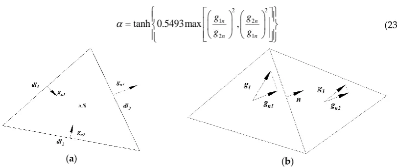
(20) where gni = upwind bed-load transport contribution of each neighboring element, across each elementedge. The schematic diagram of the element is shown [Fig. 1(a)].
In this work, the sediment transport rate of the model is estimated based on the center of the
element. The weight format is introduced for application to the transport rate at the element interface. First, the upstream and downstream elements are identified by calculating the algebraic sum gn of
the sediment transport rate in the normal direction of the two neighboring elements.
1 2
1 1 1 1
2 2 2 2
=
bn n n
n b b x x b y y
n b b x x b y y
g g g
g g n g n g n g g n g n g n
+ = = + = = + + r r r r (21)
if gbn > 0, the upstream of element 1 is located upstream of element 2; If gbn < 0, the result is the
opposite [Fig. 1(b)]. Secondly, after the upstream and downstream elements are identified, Eq. (22) is used to calculate the sediment transport rate of the element interface (gn):
(1
)
n nup ndown
g
=
g
+ −
g
(22)where α = weight coefficient, depending on g1n / g2n, calculated by:
2 2
1 2
2 1
tanh 0.5493max n , n
n n g g g g
= (23)(a) (b)
Figure 1. (a) Schematic diagram of element; (b) Schematic diagram of element interface sediment transport rate
exact position of the wet and dry discontinuities boundary which poses a challenge to programing, whereas the other is to calculate the entire elements and adopts techniques for dry elements. The simulation used in this paper introduces the latter method. It is assumed that all elements exit at least in minimal depth (it is taken to be 1 mm in actual simulation) which can also be regarded as soil moisture content, and the error of resulting water conservation may also be allowed. Hence, the method used to compute discontinuities can be adapted for other elements. If the water depth of an element and all adjacent elements are equal to the above minimal depth, it can be regarded as the land surface. Meanwhile the element at which the wet and dry discontinuities are located must be adjacent to a land element, and the specific location of the boundary need not be determined. The numerical solution is taken to represent the element average, and the singularity of the wet and dry discontinuities disappears due to integral processing.
4. Numerical Simulation
4.1. Study Case Description
The Longxi River originates from Longchi Mountain with an elevation of 2,300 m, located in the northwest of Chengdu City in Sichuan Province, China (104˚00΄- 104˚10΄E, 28˚50΄- 29˚06΄N). Longxi River flows into Min River, which is a first grade tributary of the Yangzi River. Zipiingpu reservoir is a large hydro-junction, and the height of dam is 156 m. The fluctuating backwater area of the reservoir is located downstream of Longchi River [Fig. 2(a) and 2(b)]. The Longchi River has a drainage area of 79.0 km2, and the length of the river is 18.22km [35]. The upstream bed slops is steep with an average of 13.2% and the main channel of the upstream is narrower at approximately 8 m. The bed slope of the downstream is gentle, with an average of 4.5%. The main channel upstream is wider at approximately 25 m. The Longxi River basin experiences frequent seismic activity with large changes in topography, in which the overall terrain pattern is higher elevations in the north moving to lower elevations in the south. After the Wenchuan earthquake, a large amount of loose material particles generated by the earthquake were accumulated in the basin. Due to the steepness of the ditch bed and huge variability in terrain between the hillsides, these loose sediments have large potential energy, which objectively increases the possibility of the movement of loose sediments and facilitates the transport of loose partials into the downstream river. The upstream and downstream reaches of the Longxi River experienced different morphological changes due to the earthquake [36]. The field investigation found more boulder and less sedimentation in the upstream reach with finer sediment particles, whereas a large degree of siltation occurred in the downstream of the Longxi River [Fig. 2(c) and 2(d)]. Therefore, it is of practical significance to study the Longxi River (Zipingpu Reservoir tail) for the study of the characteristics of bed-load sediment transport in the fluctuating backwater area.
(c) (d)
Figure 2. The location and survey area of the current study. (a) A shows Map of China, whereas B is Sichuan Province and C is a map, showing the Longxi River (Zipingpu reservoir tail); (b) Satellite map of Longxi river (Zipingpu reservoir tail) in 2018; (c) Onsite view of the downstream reach of Longxi River (Zipingpu reservoir tail) in 2017; (d) Onsite view of the upstream reach of Longxi River (Zipingpu reservoir tail) in 2017.
There are few accurate hydrological data and grain size distribution data of the Longhe River (Zipingpu reservoir tail) because of the many natural disasters that have impacted the area. According to the relevant discharges estimates, the flood discharge of 10-, 50- and 100-year frequencies of Longxi River are approximately 386 m3s-1, 669 m3s-1 and 795 m3s-1, respectively. In this work, the typical flood processes of 10- and 50-year frequencies were modeled [Fig. 3(a)]. In addition, the grain size distribution of numerical simulation was scaled with the size of physical model [Fig. 3(b)]. And the average and median particle sizes were Dm=37.01 mm and D50=23.64 mm, respectively.
0 10 20 30 40 50
0 100 200 300 400 500 600 700
Dischar
ge
(m
3/s)
Time (hour)
10-year frequency 50-year frequency
1 10 100
0 10 20 30 40 50 60 70 80 90 100
perc
ent
fin
er (%
)
Grain size (mm)
(a) (b)
Figure 3. (a) Flood processes of 10- and 50-year frequencies; (b) Grain size distribution of numerical simulation.
The point values of the variables at the element faces were reconstructed from the element averaged values on unstructured grids based on real measured topographic data of the Longhe River
(Zipingpu reservoir tail) in 2016, Eq. (24) represents the computation of above reconstruction
3
3 1
1
1 3 1 3 ij
i ij
j
ij j
A
x x
A =
=
=
where i = the point number at element faces j; j = the element number; xi = the point value i of physical
variables at element faces j; xij = element averaged values i of physical variables at element faces j; Aij
= the element j area. Both configurations are simulated on a 2D triangular unstructured mesh composed of 20583 elements and 10556 nodes. A detailed view of the mesh is shown in Fig. 4.
Figure 4. (a) Mesh of the entire simulation area; (b) detailed view of the mesh of bed.
4.2. Valdation Test
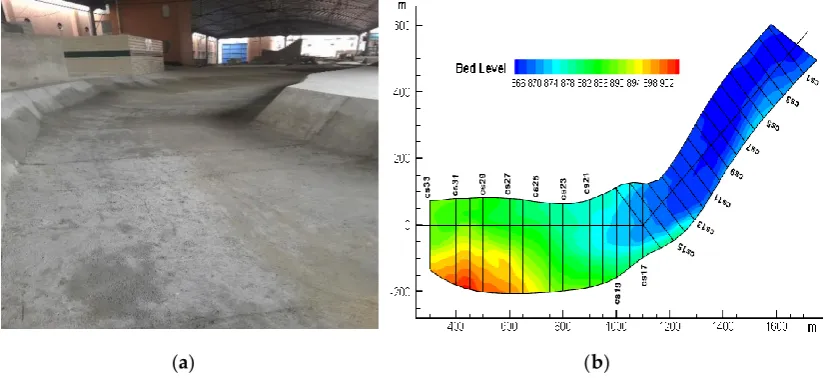
The physical model was built by the State Key Laborary of Hydraulics and Mountain River Engineering (SKLH) at Sichuan University with a 1:50 scale, based on actual topography measured in 2016 [Fig. 5(a)]. The simulation range of the physical model is from Suping Village in downstream of Longhe River to the Zipingpu reservoir tail. The length of the physical model is 2,150 m, including the numerical simulation calculation area. Numerical simulation was applied to the same sections of the fluctuating backwater area [Fig. 5(b)].
(c) (d)
(e)
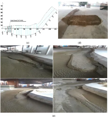
Figure 5. (a) Physical model developed by the State Key Laboratory of Hydraulics and Mountain River Engineering (SKLH) of Sichuan University; (b) Layout of measuring sections; (c) The position of the initial paved sediments of the physical model; (d) The local schematic of the initial paved sediments of the physical model;(e) Test to validate the physical model.
400 500 600 700 800 900 1000 870 875 880 885 890 895 Elevatio n ( m) Distance (m) river talweg measured value numerical value
400 500 600 700 800 900 1000
870 875 880 885 890 895 Elevatio n ( m) Distance (m) river talweg measured value numerical value
(a) (b)
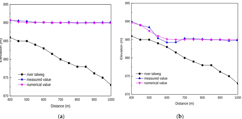
Figure 6. The water level of the river talweg in longitudinal section and the horizontal distance, which is the distance from the reference section CS39. (a) The upstream discharge = 707.1 m3s-1, the
downstream water level = 890 m; (b) The upstream discharge = 707.1m3s-1, the downstream water
level = 885 m.
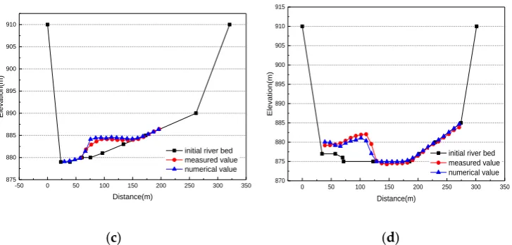
A number of experiments of sediment transport were also conducted to improve the credibility of the results of the current study. The sediment transport was verified by simulated of the above water flow boundaries, and the sediments were laid artificially between the CS36 and CS33 sections upstream of the physical model [Fig 5(c) and 5(e)]. The total amount of simulated sediments in the middle and upper reaches was limited to 150,000 m3.During the test, all sediments laid in the upstream reach were transported downstream by water flow, and no sediment remained above section CS33 [Fig 5(e)]. Fig. 7 shows a comparison between the numerical simulation results and physical model measurement as the morphologies of two randomly-chosen cross sections of the sediment of the above two schemes. The comparison illustrates that the simulation results are consistent with the results of the experiment test and that a certain minor error of sedimentation thickness exists of approximately average 0.15 m - 0.24 m. The numerical sediment transport model can therefore be regarded as credibly validated by the physical model.
0 100 200 300 400 500 600 880 885 890 895 900 905 910 915 920 Elev ati on(m) Distance(m)
initial river bed measured value numerical value
0 50 100 150 200 250 300
875 880 885 890 895 900 905 910 915 Elevatio n( m) Distance(m)
initial river bed measured value numerical value
-50 0 50 100 150 200 250 300 350 875
880 885 890 895 900 905 910
Elevatio
n(
m)
Distance(m)
initial river bed measured value numerical value
0 50 100 150 200 250 300 350
870 875 880 885 890 895 900 905 910 915
Elevatio
n(
m)
Distance(m)
initial river bed measured value numerical value
(c) (d)
Figure 7. The x-coordinate represents the distance from left to right of the varied river cross section and the y-coordinate represents the elevation of river bed. (a) The compared elevation of CS29 when the upstream discharge = 707.1 m3 s−1 and the downstream water level = 890 m; (b) The compared
elevation of CS22 when the upstream discharge = 707.1 m3 s−1 and the downstream water level = 890
m; (c) The compared elevation of CS24 when the upstream discharge = 707.1m3/s and the downstream
water level = 885 m; (d) The compared elevation of CS20 when the upstream discharge = 707.1 m3 s−1
and the downstream water level = 885 m;
4.3. Evaluation of Morphological Bed Changes in the Fluctuating Backwater Area
According to actual operation of reservoirs, this section presents three practical applications for which the numerical scheme presented by the current study is particularly relevant and suitable. The three applications concern the reservoir storage, the reservoir drawdown and the continuous flood process, which reflect the regularity of the sedimentation transport in the fluctuating backwater area of the reservoir modeled by the 2D hydrodynamic and sediment transport numerical model with the variation of water and sediment.
4.3.1. Type 1: reservoir storage
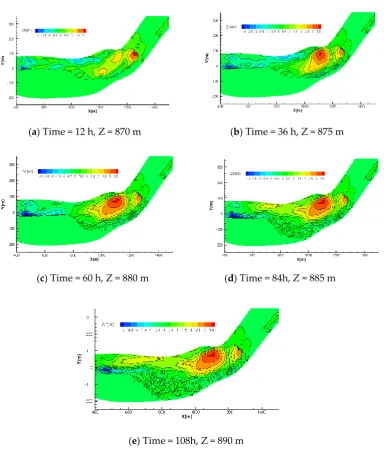
The reservoir storage is usually increased after flood conditions in which the discharge of flow is increased and sediment transport is elevated. In this type, the upstream is set to 386 m3s-1 as the steady flood discharge of 10-year frequency of Longxi River. The downstream elevation set to vary uniformly with time within the 870 m to 890 m. The upstream sediment was set the discharge of bed-load. To show the overall trend and local characteristics, the reservoir sedimentation plane morphology is displayed with the variation in contour of bed elevation.
(a) Time = 12 h, Z = 870 m (b) Time = 36 h, Z = 875 m
(c) Time = 60 h, Z = 880 m (d) Time = 84h, Z = 885 m
(e) Time = 108h, Z = 890 m
Figure 8. Variation in the contours of bed elevation under the same upstream discharge and different downstream water levels of reservoir storage; (a) Time of simulation is 12 h and downstream water level is 870 m; (b) Time of simulation is 36 h and downstream water level is 875 m; (c) Time of simulation is 60 h and downstream water level is 880 m; (d) Time of simulation is 84 h and downstream water level is 885 m; (e) Time of simulation is 108 h and downstream water level is 890 m.
400 600 800 1000 1200 1400 870
875 880 885
Elevatio
n (
m)
Distance (m)
initial river bed 870 m 875 m 880 m 885 m 890 m
Figure 9. The river bed elevation of river talweg in longitudinal section during reservoir storage, and the horizontal distance is the distance from the reference section CS39.
4.3.2. Type 2: reservoir drawdown
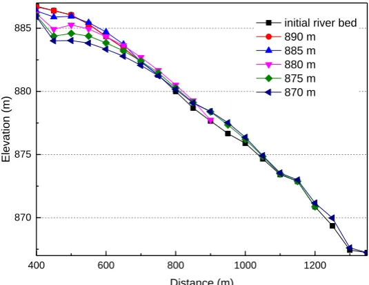
During the reservoir full flood period, the water level in front of the dam needs to gradually drop due to power generation, etc., which leads to erosion in the fluctuating backwater area. This process is simulated within this type. The final simulation results of reservoir storage was used as the initial topography in this simulation. The upstream flow was set as 189.6 m3s-1 as a steady mean flood discharge of Longxi River. The downstream elevation was set uniformly vary with time within a range of an initial 890 m to 870 m. The upstream sediment load was set zero.
(a) Time = 48 h, Z = 885 m (b) Time = 72 h, Z = 880 m
(c) Time = 96 h, Z = 875 m (d) Time = 120 h, Z = 870 m
Figure 10. The variation in the contours of bed elevation under the same upstream discharge and different downstream water levels during reservoir drawdown; (a) Time of simulation is 48 h and downstream water level is 885 m; (b) Time of simulation is 72 h and downstream water level is 880 m; (c) Time of simulation is 96 h and downstream water level is 875 m; (d) Time of simulation is 120 h and downstream water level is 870 m.
As illustrated by Fig. 11 (the same as type 1), there is almost no scouring effect on the river bed by backwater when the downstream water level is 890 m. Scouring of the river bed between CS31 and CS39 begins when the downstream water level drops to 885 m, which produces a large of sediment in the backwater area and forms a triangular sedimentation pattern. The erosion of the river-bed gradually evolves to downstream, and the triangular sedimentation also continue to move to downstream as the downstream water level drops. Meanwhile, the triangular sedimentation pattern is stretched with the evolution of erosion and siltation. The slope of the longitudinal section of the river bed in the fluctuating backwater area is generally gradually reduced.
400 600 800 1000 1200
870 875 880 885
Elevatio
n (
m)
Distance (m)
initial river bed 890 m 885 m 880 m 875 m 870 m
Figure 11. The river bed elevation of river talweg in longitudinal section during reservoir drawdown, and the horizontal distance is the distance from the reference section CS39.
4.3.3. Type 3: continuous flood process
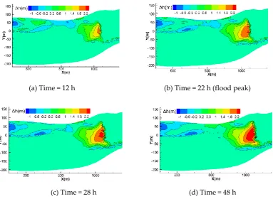
m for Case B. The upstream sediment was employed in the discharge of bed-load. Fig. 12 shows the reservoir sedimentation plane morphology with the variation in the contour of bed elevation. Numerical results are summarized in Fig. 12 for Case A and Fig. 13 for Case B. These figures include the results for variation in bed elevation at different times (Time = 12 h, 22 h, 28 h, 48 h).
Fig. 12(a) of Case A shows that sedimentation appears near CS18 (x = 1000 m) and with scouring of the upstream river-bed. Because of the minimal discharge from upstream, some sediment carried by flow is deposited in CS26 (x = 650 m). It’s clear that erosion occurs near CS23 (x = 800 m) where the channel is narrower and consequently flow velocity is higher. As the simulation time progresses, erosion gradually moves downstream, and the sediment supplied by upstream gradually increases. A maximum discharge occurs as 22 h (flood peak) in Fig.12 (b), and the forward slope of sedimentation halts. The elevation of sedimentation rises and the tail is kept back. The triangular sediment is deposited near CS21 (x = 800 m) when the downstream water level is 880 m. The elevation of sedimentation rises and the tail back is not obvious compared to that at 875 m up to 22 h (Fig. 13 of Case B).
(a) Time = 12 h (b) Time = 22 h (flood peak)
(c) Time = 28 h (d) Time = 48 h
Figure 12. The variation in the contours of bed elevation of Case A under a typical continuous flood process with the flood discharge of 50-year frequency set at approximately 669 m3s-1 and the
downstream water level as 875 m in the fluctuating backwater area. (a) Time of simulation is 12 h; (b) Time of simulation is 22 h; (c) Time of simulation is 28 h; (d) Time of simulation is 48 h.
(c) Time = 28 h (d) Time = 48 h
Figure 13.The variation in the contours of bed elevation of Case B under a typical continuous flood process and the flood discharge of 50-year frequency set to approximately 669 m3s-1
and the downstream water level as 880 m in the fluctuating backwater area. (a) Time of simulation is 12 h; (b) Time of simulation is 22 h; (c) Time of simulation is 28 h; (d) Time of simulation is 48 h.
Fig. 14 shows the river bed elevation of river talweg in longitudinal section under a typical continuous flood process for all investigated times, including Fig. 14(a) corresponding to Case A and Fig. 14(b) corresponding to Case B. The figures show that the duration of sedimentation for Case A is longer than that for Case B.
The location and bed morphology of the end of the backwater varies under the same inlet flow conditions and different downstream water levels. The location and direction of upstream flow varies under different locations and morphology, resulting in flow conditions under which there are large differences in sedimentation. Therefore, the sedimentation under Case A occurs close to the right bank of the river, whereas sedimentation under Case B occurs close to the left bank of the river. Because the location of sedimentation under Case A is less constrained than that under Case B, the sedimentation shape under Case A is short and wide, whereas that under Case B is long and narrow. In short, there is an element of randomness in the location and morphology of sedimentation effected by the downstream water level and the fluctuating backwater.
400 600 800 1000
875 880 885
Elevatio
n (
m)
Distance (m)
initial river bed 12h 22h 28h 48h
400 600 800
880 885
El
evation
(
m)
Distance (m)
initial river bed 12h 22h 28h 48h
(a) (b)
Figure 14. The river bed elevation of river talweg in longitudinal section under a typical constant flood process, and the horizontal distance is the distance from the reference section CS39. (a) Case A: the flood discharge of 50-year frequency set to approximately 669 m3s-1 and the downstream water
level as 875 m; (b) Case B: the flood discharge of 50-year frequency set to approximately 669 m3s-1and
5. Conclusions
This paper presents a numerical strategy to deal with bed-load erosion and deposition in the fluctuating backwater area using the shallow-water equations and Exner equation solvers. The 2D shallow water hydrodynamic model of the fluctuating backwater area was calculated based on the finite volume method of a Godunov scheme. The bed-load transport and river-bed deformation were calculated using an uncoupled saturated sediment transport model. The entire modelling software was written using FORTRAN programing language. This study used the Longxi River, a small stream in Dujiangyan located in Sichuan Province, as the case study research reach.
To validate the performance of the numerical model, a physical model in was constructed at the SKLH of Sichuan University, and was applied for two cases studies. The average water level of river talweg in longitudinal section and the river-bed morphologies of two randomly-chosen cross sections of the sediment of numerical simulation were consistent with the measured value in physical model, which means numerical model is believable. Actual conditions of the operation of the reservoir were studied to reflect the characteristics of bed-load erosion and deposition in the fluctuating backwater area, including three types: reservoir storage, drawdown of the reservoir, and continuous flooding process with different water levels. The following results were obtained within the present work:
• The sedimentation in the fluctuating backwater area is mainly deposited in the main channel and the elevation difference between beach and channel decreases with time. In the river bend, the sedimentation is mainly concentrated on the convex bank, readily resulting in the growth of a convex bank beach. Although the concave bank also experiences siltation, the quantity is relatively minor.
• During the drawdown period of the reservoir, the original sedimentation is scoured, with scouring concentrated over a small width. The flow gradually erodes a deep channel in the river-bed, forming compound channels with a beach and multiple channels, which reshapes the channel of the low flow period. The deposition of bed-load from upstream to downstream and the slope of the longitudinal section of the river bed in the fluctuating backwater area is generally gradually reduced.
• There is an element of randomness in the location and morphology of sedimentation due to the effected of the downstream water level lead and fluctuating backwater. Under type 3, the location and bed morphology of the end of the backwater varies under the same inlet flow conditions and different downstream water levels. The location and direction of upstream flow is changed under differences in location and morphology, resulting in large differences in sedimentation under different flow conditions.
Author Contributions: Ming Luo and Heli Yu designed and carried out the simulations and wrote the paper; Er Huang contributed to the conception of the study; Rui Ding analyzed the data and validation; Xin Lu contributed physical model data.
Funding: This research was funded by the National Natural Science Foundation of China (No. 51539007).
Acknowledgments: The work was supported by the State Key Laboratory of Hydraulics and Mountain River Engineering (SKLH) at Sichuan University through the program Science, and the National Natural Science Foundation of China and code 51539007. The authors are also grateful to all teachers and students of SKLH.
Conflicts of Interest: The authors declare no conflict of interest.
References
1. Kondolf, GM; Gao, YX; Annandale, GW; Annandale, GW; Morris, GL. Sustainable sediment management in reservoirs and regulated rivers: Experiences from five continents. Earths Future, 2014, 2(5):256-280. 2. Kondolf, GM; P Pinto. The social connectivity of rivers. Geomorphology, 2017, 277:182-196.
3. Han, QW. Sedimentation in Reservoir. Beijing, China Science Publishing & Media Ltd. 2003.
5. Radoane, M; Radoane, N. Dams, sediment sources and reservoir silting in Romania. Geomorphology, 2005, 71(2): 112-125.
6. Caputo, M; Carcione, JM. A memory model of sedimentation in water reservoirs. Journal of Hydrology, 2013, 476(1):426-432.
7. Hanmaiahgari PR; Gompa NR; Pal D; Pu JH. Numerical modeling of the Sakuma Dam reservoir sedimentation. Natural Hazards, 2018, 91(3):1075-1096.
8. Ahn, J; Yang, C. Determination of recovery factor for simulation of non-equilibrium sedimentation in reservoir. International Journal of Sediment Research, 2015, 30(1):68-73.
9. Renyi Xu, Deyu Zhong, Baosheng Wu. A large time step Godunov scheme for free-surface shallow water equations. Chin. Sci. Bull. 2014, 59(21):2534–2540.
10. Esmaeili, T; Sumi, T; Kantoush, SA. Three-Dimensional Numerical Study of Free-Flow Sediment Flushing to Increase the Flushing Efficiency: A Case-Study Reservoir in Japan. Water, 2017, 9(11).
11. Fischer-Antze, T; Olsen, NRB; Gutknecht, D. Three-dimensional CFD modeling of morphological bed changes in the Danube River. Water Resources Research, 2008, 44(9).
12. Faghihirad, S., Lin, Binliang and Falconer, Roger Alexander. 3D layer-integrated modelling of morphodynamic processes near river regulated structures. Water Resources Management. 2017, 31(1): 443-460.
13. Francesco Gallerano, Giovanni Cannata, Francesco Lasaponara, Chiara Petrelli. A new three-dimensional finite-volume non-hydrostatic shock-capturing model for free surface flow. Journal of Hydraulics: 2017,29(4):552-566.
14. Victoria, BA; Rzetala, MA. Condition of Relief formation of Bottom and Banks in Upper part of Bratsk Reservoir, Russia. In Proceedings of the 14th International Multidisciplinary Scientific Geoconference, Albena, Bulgaria, 17-26, 2014.
15. Jagus, A; Rzetala, MA; Rzetala, M. Water storage possibilities in Lake Baikal and in reservoirs impounded by the dams of the Angara River cascade. Environmental Earth Sciences, 2015,73(2): 621-628.
16. Lu, HR; Li, SS; Guo, JS. Modeling Monthly Fluctuations in Submersion Area of a Dammed River Reservoir: A Case Study. Journal of the American Water Resources Association. 2013, 49(1): 90-102.
17. Huang, Y; Yasarer, LMW; Li, Z. Air-water CO2 and CH4 fluxes along a river-reservoir continuum: Case study in the Pengxi River, a tributary of the Yangtze River in the Three Gorges Reservoir, China. Environmental Monitoring and Assessment, 2017, 189(5).
18. Lu, YJ; Zuo, LQ; Ji, RY; Liu, HX. Deposition and erosion in the fluctuating backwater reach of the Three Gorges Project after upstream reservoir adjustment. International Journal of Sediment Research. 2010, 25(1):64-80.
19. Han QW, He MM. Bed Load Agration in Reservoir and Deposition in Variable Backwater Region. Journal of Sediment Research, 1986(2): 1-16.
20. Xie JH, Li YT. Influence of sediment deposition on the navigation conditions in the fluctuating backwater region of the Three Gorges Reservoir. Journal of Hydraulic Engineering, 1988, (7): 18-26.
21. Xie BL. Fluvial process in fluctuating backwater reach of the Three-Gorge Reservoir. Journal of Hydraulic Engineering, 1994, (4): 50-54.
22. Lu YJ, Xu CW, Zuo LQ, et al. Changes of sediment deposition and erosion at Chongqing Reach in backwater area of Three Gorges Project. In Proceedings and Monographs in Engineering Water and Earth Sciences, Lisbon, Portugal, 06-08 Sep 2006.
23. Lu YJ, Zuo LQ, Ji RY, et al. Changes of sediment deposition and erosion at Chongqing reach in backwater area of Three Gorges Project after reservoir adjusting of the upstream in the Yangtze River. Advances in Water Science, 2009, 20(3): 318-234.
24. Liu, WL; Liu, XF; Ping, KJ. Research on Waterway Regulation of Fluctuating Backwater Zone of Ankang Hydro-junction. In proceedings of the 5th International Conference on Civil Engineering and Transportation, Guangzhou, Peoples R China, 28-29 Nov 2012.
25. Wang D, Liu X, Ji Z, et al. Influence of flocculation on sediment deposition process at the three gorges reservoir. Water Sci Technol, 2015, 73(10):873–880.
27. Zhou, Guo-dong and Liu, Qiong-yi. Non-uniformity coefficient effects in alluvial streams. J. HydrodynamicZs. , 2003, 18(5), 576-583.
28. Gallerano, F; Cannata, G; De Gaudenzi, O; Scarpone, S. Modeling bed evolution using weakly coupled phase-resolving wave model and wave-averaged sediment transport model. Coastal Engineering Journal. 2016, 58(3).
29. Chien Ning, and Chao-Hui Wan, Z. Mechanics of sediment transport.” ASCE, Reston, 1999. 30. Toro E F. Shock-capturing methods for free-surface shallow flows. Wiley and Sons Ltd, 2001.
31. Toro E F. Riemann solvers and numerical methods for fluid dynamics. A practical introduction. Springer Science & Business Media, 2003.
32. Pan Cun-hong, Dai Shi-qiang and Chen Sen-mei. Numerical Simulation for 2D Shallow Water Equations by Using Godunov-type Scheme with Unstructured Mesh. J. of Hydrodynamics, 2006, 18 (4), 475-480. 33. Gallerano, F; Cannata, G; Lasaponara, F. Numerical simulation of wave transformation, breaking and
runup by a contravariant fully non-linear Boussinesq equations model. Journal of Hydrodynamics. 2016, 28(3): 379-388.
34. Cannata, G; Lasaponara, F; Gallerano, F. Non-Linear Shallow Water Equations numerical integration on curvilinear boundary-conforming grids. WSEAS Transactions on Fluid Mechanics. 2015, 10: 13-25. 35. Ang Zhang, Haiyun Shi, Tiejian Li. Analysis of the Influence of Rainfall Spatial Uncertainty on
Hydrological Simulations Using the Bootstrap Method. Atmosphere, 2018, 9(2), 1-24.

![Fig. 10. When downstream water level is 885 m [Fig. 10(a)], the upstream river bed is scoured and the The variation in the contours of bed elevation during reservoir drawdown are summarized by river channel is reshaped, thereby establishing the river morph](https://thumb-us.123doks.com/thumbv2/123dok_us/1043632.1604623/15.595.161.434.79.292/downstream-variation-contours-elevation-reservoir-summarized-reshaped-establishing.webp)