Mining data from CFD simulations for aneurysm and carotid bifurcation
models
N.Janković1
, M.Radović2, D.Petrović2, N.Zdravković1 and N.Filipović2,3
1
Faculty of Medical Sciences, Svetozara Markovica 69, Kragujevac, Serbia
2
Bioengineering Research and Development Center- BioIRC, Prvoslava Stojanovica 6, Kragujevac, Serbia
Email: [email protected]
3
Faculty of Engineering, Sestre Janjic 6, Kragujevac, Serbia Email: [email protected]
Abstract
Arterial geometry variability is present both within and across individuals. To analyze the influence of geometric parameters, blood density, dynamic viscosity and blood velocity on wall shear stress (WSS) distribution in the human carotid artery bifurcation and aneurysm, the computer simulations were run to generate the data pertaining to this phenomenon. In our work we evaluate two prediction models for modeling these relationships: neural network model and k-nearest neighbor model. The results revealed that both models have high prediction ability for this prediction task. The achieved results represent progress in assessment of stroke risk for a given patient data in real time.
1. Introduction
After heart disease and cancer, the third most common cause of death is stroke. The carotid bifurcation stenosis is a significant cause of stroke, producing the infarction in the carotid region by embolization or thrombosis at the site of narrowing. The thrombosis development and embolization is conditioned by the local hemodynamics which can be investigated experimentally and/or by computer modeling.
There are many factors which increase the stroke risk like age, systolic and diastolic hypertension, diabetes, cigarette smoking, etc. It has been shown that changes of the geometrical vessel dimensions in the region of the carotid artery bifurcation certainly affect the blood flow and may lead to stenosis process [Schulz and Rothwell 2001], [Schulz and Rothwell 2001].
Kolachalama used Bayesian Gaussian process emulator to access the relationship between geometric parameters and Maximal Wall Shear Stress (MWSS) and to obtain geometries having maximum and minimum values of the output MWSS [Kolachalama et al. 2007].
Large changes in the magnitude of maximal wall shear stress can play a role in the embolic mechanism by which carotid lesions can induce stroke [Lorthois et al. 2000].
potential for modeling relationship between geometric parameters of the carotid bifurcation and the MWSS [Radovic et al. 2010].
The rupture of aneurysm, can cause severe hemorrhage, other complications or death. It has been shown that aneurysm growth occurs at regions of low WSS [Boussel et al. 2008].
An example of data mining application in computational fluid dynamics (CFD) has been shown in Filipovic‘s paper [Filipovic et al. 2011]. In this paper, the focus was to combine the CFD and data mining methods for the estimation of the wall shear stresses in an abdominal aorta aneurysm under prescribed geometrical changes.
In the present work, we evaluate two data mining prediction models (NN model and k-NN model) and test their performance in modeling the relationship between geometric factors, blood density, dynamic viscosity and blood velocity and WSS distribution. The basic idea is to construct probabilistic models for the input variables which will replace classical CFD calculations and to give the output of interest very quickly.
The present approach can be viewed as a computer-based data mining strategy which extracts useful information and synthesizes interesting relationships from data sets generated by running computer simulations on selected cases. The human carotid artery bifurcation and aneurysm were chosen for analysis.
2. Methodology
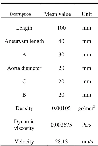
2.1 Data Sets for Modeling WSS Distribution
Description Mean value Unit
Length 100 mm
Aneurysm length 40 mm
A 30 mm
Aorta diameter 20 mm
C 20 mm
B 20 mm
Density 0.00105 gr/mm3
Dynamic
viscosity 0.003675 Pa∙s
Velocity 28.13 mm/s
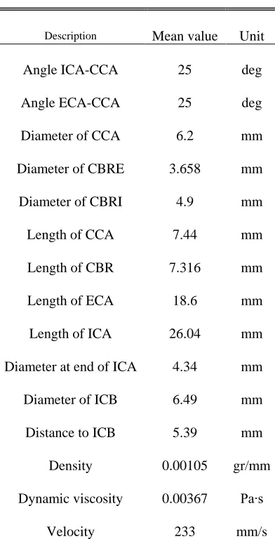
Description Mean value Unit
Angle ICA-CCA 25 deg
Angle ECA-CCA 25 deg
Diameter of CCA 6.2 mm
Diameter of CBRE 3.658 mm
Diameter of CBRI 4.9 mm
Length of CCA 7.44 mm
Length of CBR 7.316 mm
Length of ECA 18.6 mm
Length of ICA 26.04 mm
Diameter at end of ICA 4.34 mm
Diameter of ICB 6.49 mm
Distance to ICB 5.39 mm
Density 0.00105 gr/mm
Dynamic viscosity 0.00367 Pa∙s
Velocity 233 mm/s
Table 2. The average values of input parameters for carotid bifurcation model
Fig. 1. Geometrical parameters of aneurysm model: ‘Length‘is the parameter which defines the total horizontal projection of the generated aneurysm model; ‗A‘is the height of the arc of central line; ‗Aorta diameter‘ is the abdominal aorta diameter; ‗B‘ is the radius from the central
line to the inner wall of the aneurysm; ‗C‘ is the radius from the central line to the outer wall of
the aneurysm; ‗Aneurysm length‘ is an average length of the aneurysm
Fig. 2. Geometrical data for the carotid artery model. The abbrevations here are: CCA – common carotid artery, CBR – carotid bifurcation region, CBRE – carotid bifurcation region external, ECA- external carotid artery, CBRI- carotid bifurcation region internal, ICA- internal
carotid artery, ICB- internal carotid bulbus
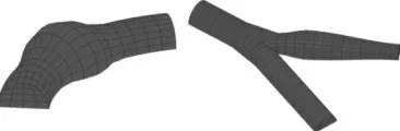
FE model of aneurysm contains 375 nodes from which 195 lie on surface. On the other hand, FE model of carotid bifurcation contains 1854 nodes from which 642 lie on surface. By using CFD simulations WSS values are calculated in surface nodes for each of 4779 different geometries for both models. FE models of aneurysm and carotid artery bifurcation are shown on Figure 3.
2.2 Multilayer Perceptron Neural Network
Multilayer perceptron (MLP) neural network is composed of simple elements called neurons. The basic structure of the MLP, consists of one or more hidden layers and an output layer.
The objective of the training is to find a set of weights and biases that minimize the error between the neural network predictions and the desired outputs. There are different learning algorithms. The back-propagation algorithm [Rumelhart et al. 1986] has been the most commonly used training algorithm. The basic algorithm is a gradient descent method in which the network weights and biases are moved along the negative performance function. An iteration of this algorithm can be written as:
dX dperf lr X
(1)
where X represents weight and bias variables of the network,
lr
is learning rate andperf
is performace function which defines how much real outputs disagree with predicted ones (mean squared error for example).It has problems with local minima and slow convergence. In the literature, a number of variations of the standard algorithm have been developed [Haykin 1999]. In this study we used backpropagation algorithm with momentum and adaptive learning rate. Each variable is adjusted according to gradient descent with momentum:
dX dperf m lr X m
X c prev c
(2)
where
m
cis momentum constant and
X
prev is the previous change of the weight or bias. Foreach epoch, if performance decreases toward the goal, then the learning rate is increased by the
inc
lr
factor. If performance increases by more than themax
inc factor, the learning rate isadjusted by the factor
lr
decand the change that increased the performance is not made. Thevalues of
m
c,lr
inc,lr
decandmax
incare given in Table III.c
m
lr
inclr
decmax
inc0.9 1.05 0.7 1.04
Table 3.
m
c,lr
inc,lr
decandmax
incValues Used for MLP TrainingMLP with as few as one single hidden layer is indeed capable of universal approximation in a very precise and satisfactory sense [Hornik 1991].
2.3 K-Nearest Neighbors Algorithm
For regression problems the mean target variable value from the set of nearest neighbors is predicted:
k i i xc
k
c
11
(3)where
k
is the number of nearest learning examples which influence the prediction of k-NN algorithm.Type of distance measure has big impact on determining which set of learning examples are closest to the new example. In the most cases, Euclidean distance is used:
a i j i l i jl t d v v
t D 1 2 , ,, ) ( ) , ( (4)
In (4),
D
(
t
l,
t
j)
is Euclidean distance between 2 examplest
landt
j, anda
is the totalnumber of attributes.
Before calculating Euclidean distance all attributes are scaled to the [0,1] interval. For continuous attributes the distance between two attributes
v
i,l andv
i,j is defined as:j i l i j i l
i v v v
v
d( ,, , ) , ,
(5)
3. Results
In this paper we used MLP neural networks trained with backpropagation algorithm and k-NN algorithm for predicting wall shear stress distribution for the two different FE models. The problem that we are solving is multi-target prediction problem, and because of that for each surface node of the models we created one MLP. This means that our model consists of 195 different neural networks in case of aneurysm model and 642 different neural networks in case of carotid bifurcation model, one for each surface node. For training this model and k-NN model we randomly chose 70% of the total data (3346 learning examples). Remaining 30% of data is used for testing (1433 testing examples).
MLPs with 5 neurons in hidden layer, bipolar sigmoid activation functions in hidden neurons and linear activation function in the output neuron are used. The stopping criterion was defined as the maximum number or learning epochs (1000). Input layer has nine input neurons (in case of aneurysm model) and fifteen input neurons (in case of carotid bifurcation model) corresponding to input parameters (see Tables I and II). The output layer consists of one neuron corresponding to WSS value of the node for which MLP is created.
k-NN model predicts the target values that are averaged from the 5 most similar learning examples (nearest neighbors) in the problem space.
We evaluated the performance of the models by computing their relative mean squared error (RMSE). RMSE is computed as a sum of the squared differences between the true and the predicted values of the outputs for all of 1433 testing examples and is afterwards normalized with the sum of the squared errors of the default predictor (i.e. a model which always predicts average values of the outputs).
n i i j i jj f f
ERR 1 2 , , ˆ (6)
where
n
is the number of surface nodes (195 or 642),f
ˆ
j,i is the predicted WSS value for i-thnode for j-th example and
f
j,i is the true value of WSS for i-th node of j-th example.In the same way, squared error for default predictor for j-th learning example is calculated as:
n i i i jj f f
ERR
1
2
,
(7)
where
f
i is the average value of WSS for i-th node among training examples:
Ntrainj i j train i
f
N
f
1 ,1
(8)where
N
train is the number of training examples (3346).Finally, RMSE is calculated as:
test test N j j N j j ERR ERR RMSE 1 1 (9)where
N
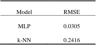
test is the number of testing examples (1433).The lower RMSE is, the more accurate the model is. The RMSE values for the tested models are shown in Tables IV and V for aneurysm and carotid bifurcation model respectively.
Model RMSE
MLP 0.0351
k-NN 0.1008
Table 4. Relative Mean Squared Error of the Tested Models for Aneurysm Model
Model RMSE
MLP 0.0305
k-NN 0.2416
Figures 4 and 5 show calculated and predicted WSS distribution for three randomly chosen test examples for aneurysm and carotid bifurcation models (Other results are not shown here).
Fig. 4. WSS distribution for aneurysm model (3 randomly chosen geometries out of 1433 testing ones are shown): left-calculated, middle-MLP predicted, right-k-NN predicted [units Pa]
Fig. 5. WSS distribution for carotid bifurcation model (3 randomly chosen geometries out of 1433 testing ones are shown): left-calculated, middle-MLP predicted, right-k-NN predicted
[units Pa]
4. Conclusion
This work presented an application of data mining methodology to a hemodynamic problem in which the relationship between geometric parameters, blood density, dynamic viscosity and blood velocity of the human carotid bifurcation and aneurysm, and the wall shear stress distribution was modeled. The results obtained from computer simulations were used as training data to evaluate two different regression models, which both exhibited capabilities of being used for this task. The neural network model showed better results than k-NN model. The achieved results can be used to aid the assessment of stroke risk for a given patient‘s data in real time. Further research will focus on real life situations where applicability of created data mining applications will be tested on real patient data. Also, other regression models like support vector machines (SVM) and linear regression will be created and tested.
5. Acknowledgment
Извод
Повезивање података добијених из компјутерских симулација за
моделе анеуризме и каротидне бифуркације
Н.Јанковић1
, M.Радовић2, D.Петровић2, N.Zdravković1 and N.Filipović2,3
1
Faculty of Medical Sciences, Svetozara Markovica 69, Kragujevac, Serbia
2
Bioengineering Research and Development Center- BioIRC, Prvoslava Stojanovica 6, Kragujevac, Serbia
Email: [email protected]
3
Faculty of Engineering, Sestre Janjic 6, Kragujevac, Serbia Email: [email protected]
Резиме
Варијабилност геометрије артеријског система је особина индивидуалности. Да би се анализирао утицај геометријских параметара, густине крви, динамичке вискозности и брзине крви на дистрибуцију смичућег напона зида у бифуркацији и анеуризми људске каротидне артерије, компјутерске симулације су урађене да би се генерисали подаци који се односе на овај феномен. У овом раду, оцењујемо два предикциона модела за моделирање ових релација: модел неуронске мреже и алгоритам к-најближих суседа. Резултати су показали да оба модела имају велике могућности предвиђања. Остварени резултати представљају прогрес у процени ризика од срчаног удара за испитиване пацијенте у реалном времену.
References
D.E. Rumelhart, G.E. Hinton, R.J. Williams, ―Learning internal representations by error propagation,‖ MIT Press, Cambridge, MA, USA, 1986, pp. 318-362.
I. Kononenko, M. Kukar, "Machine learning and data mining," Horwood Publishing Chichester, UK, 2007.
K. Hornik, ―Approximation capabilities of multilayer feedforward networks,‖ Neural network, vol. 4, no.2, pp. 251–257, 1991.
L. Boussel, V. Rayz, C. McCulloch, A. Martin, G. Acevedo-Bolton, M. Lawton, R. Higashida, W.S. Smith, W. Young, D. Saloner, ―Aneurysm growth occurs at region of low wall shear stress: Patient-specific correlation of hemodynamics and growth in a longitudinal study,‖ Stroke, vol. 39, no. 11, pp. 2997–3002, 2008.
M. Radovic, N. Filipovic, Z. Bosnic, P. Vracar and I. Kononenko, ―Mining Data from Hemodynamic Simulations for Generating Prediction and Explanation Models,‖ Conference paper, ITAB 2010 Corfu-Greece.
N. Filipovic, M. Ivanovic, D. Krstajic, M. Kojic, ―Hemodynamic Flow Modeling Through an Abdominal Aorta Aneurysm Using Data Mining Tools,‖ Information Technology in Biomedicine, IEEE Transactions on, Vol. 15, No. 2, pp. 189 – 194, 2011.
S. Lorthois, P.Y. Lagree, J.P. Marc-Vergnes, F. Cassot, ―Maximal wall shear stress in arterial stenoses: Application to the internal carotid arteries,‖ ASME Journal of Biomechanical Engineering Vol. 122, pp. 661-666, 2000.
U.G.R. Schulz, P.M. Rothwell, ―Major variation in carotid bifurcation anatomy. A possible risk factor for plaque development?,‖ Stroke, vol. 32, no. 7, pp. 2522-2529, 2001.
U.G.R. Schulz, P.M. Rothwell, ―Sex differences in carotid bifurcation anatomy and the distribution of atherosclerotic plaque,‖ Stroke, vol. 32, no. 7, pp. 1525-1531, 2001.
![Fig. 4. WSS distribution for aneurysm model (3 randomly chosen geometries out of 1433 testing ones are shown): left-calculated, middle-MLP predicted, right-k-NN predicted [units Pa]](https://thumb-us.123doks.com/thumbv2/123dok_us/8371219.1675251/9.499.166.365.323.487/distribution-aneurysm-randomly-geometries-testing-calculated-predicted-predicted.webp)
