How Many Bits Can a Flock of Birds Compute?

www.theoryofcomputing.org

How Many Bits

Can a Flock of Birds Compute?

Bernard Chazelle

Received August 3, 2012; Revised October 30, 2014; Published November 13, 2014

Abstract: We derive a tight bound on the time it takes for a flock of birds to reach equilibrium in a standard model. Birds navigate by constantly averaging their velocities with those of their neighbors within a fixed distance. It is known that the system converges after a number of steps no greater than a tower-of-twos of height logarithmic in the number of birds. We show that this astronomical bound is actually tight in the worst case. We do so by viewing the bird flock as a distributed computing device and deriving a sharp estimate on the growth of its busy-beaver function. The proof highlights the use of spectral techniques in natural algorithms.

ACM Classification:F.2.0

AMS Classification:68W25

Key words and phrases:natural algorithms, dynamical systems, bird flocking, busy-beaver function

1

Introduction

In a standard flocking model,nbirds fly in the sky and modify their velocities at each time step by averaging them with those of their neighbors within a fixed distance (Figure 1). It has been shown that the system always tends to equilibrium and that the relaxation time is bounded by a tower-of-twos of heightO(logn), which is “two to the two to the two. . . ” repeated on the order of logntimes [2]. Past that worst-case limit, equilibrium is approached exponentially fast: the birds fly with constant velocities subject fast-decaying deviations. We show here that, oddly enough, this astronomical upper bound is in fact optimal.

Figure 1: Each bird averages its velocity with those of its neighbors within a fixed radius.

This work is part of an effort to understand the worst-case behavior of bird flocking viewed as a

natural algorithm. Because the actual biology of bird flying is beyond anybody’s grasp at this point, a reasonable approach is to specify an idealized model of the phenomenon that, one hopes, captures some essential aspect of the behavior. In this case, the model tries to express the birds’ uncanny ability to reach consensus about their velocities despite the ever-changing topology of their communication channels. To prove that the time to reach equilibrium can be very high, one must carefully engineer a starting configuration of the birds and show how their behavior remains essentially nontrivial for a long time. What does this mean? Because the velocities and positions of the birds can be assumed to be rational numbers, the evolution of the group can be modeled by a distributed algorithm operating over the rationals. Since it is known that the flocking algorithm will always converge, the question is: How long can it take in the worst case?

As it happens, this is equivalent to asking how many bits are required to encode the final stationary velocity of the birds. If three birds are initialized withmbits each, none of them can compute a single extra bit on their own: together, however, they can produce 2Ω(m)_{brand-new bits! It is in this sense that}

one can talk about the number of bits “computed” by a bird flock. This is similar to what is known in computational complexity as the “busy-beaver problem”: given a program, how long can it run and halt for an input of sizen? In our case, the birds never stop flying so, technically, the program never halts. The creation of new flocks does, however. Natural algorithms, by definition, never stop. Their busy-beaver functions, therefore, merely count how much time can elapse before their behaviors become trivial, i. e., fixed or asymptotically periodic.

The model and the main result. Most models of bird flocking studied in the literature follow theboids

has focused on variants of rule (i) [2–8,10–13]. This bold choice was validated recently by the empirical findings of the STARFLAG project, the most comprehensive experimental bird flocking investigation to date [1].

The model is easy to describe. We give a formal description below but a few words of explanation suffice to tell the whole story. A bird is represented by a point in Euclidean 3-space along with a three-dimensional vector indicating its velocity. For a system ofnbirds, the initial condition is thus entirely specified by 6nnumbers. The timetis discrete, so the position of a birdiat timetis given by its placementxiat timet−1 shifted by its current velocityvi; in other words, the bird’s locationxibecomes

xi+vi. To updatevi, we form an undirected graph, called theflocking network, by connecting any two

birds within unit distance by an edge, and we express the new velocity of birdiby averaging its current velocityviwith those of its neighbors in the graphs. The system reaches equilibrium when the flocking

network no longer changes. The terminology is justified by the fact that, once the network settles on a final configuration, the birds soon begin to fly (essentially) in a straight line at constant speed: from that point on, nothing of interest happens. The model is robust in that the averaging can be weighted, if so desired, and a moderate amount of decaying noise can be tolerated as well. The connected components of the flocking network are called theflocksof the system. They will typically fragment and merge in erratic ways, and it is this evolving topology that makes such systems hard to analyze.

Indeed, if the flocking network were fixed once and for all, the velocities would evolve by iterated averaging in a manner lending itself to the theory of random walks. The crux of the matter is that the flocking network may be constantly changing. If the changes were random, some of the tools for Markov chains could be rescued, but the difficulty is that the changes are endogenous. There is a feedback loop from the positions of the birds, which determine the flocking network, which in turn specifies the evolution of the velocities, which then determine the new bird positions. To show that the system always reaches equilibrium calls on tools from different areas [2]: combinatorics, linear algebra, circuit complexity, computational geometry, even elimination theory—to determine whether two birds will ever be within unit distance of each other requires root separation bounds for various characteristic polynomials.

In the field of dynamics, attraction to a fixed point is usually established by exhibiting a Lyapunov function. Because of the changing topology of the network, this approach runs into all sorts of problems here. Fortunately, proving the matching lower bound can be done entirely within the language of linear algebra. Once we engineer a starting configuration for the birds, to bound the relaxation time is a matter of monitoring the evolution of various Fourier coefficients as flocks merge together. Of course, it is the occasional presence of nonlinearities that causes the astronomical delay we seek. In the construction, the number of nonlinearities can be kept remarkably small (in fact, less than the number of birds). To see why Fourier analysis arises naturally, it is helpful to compare the transmission of information among the birds to the diffusion of heat in a medium. By choosing the right topology, we can ensure that the eigenfunctions of the Laplacian form a nice, simple set of harmonics.

We define the model formally. Givennbirds represented at timetby their position vectorx(t) = (x1(t), . . . ,xn(t))∈(R3)n, theflocking network at time t links any two birds (the nodes) within unit

For anyt>0,

(

x(t) =x(t−1) +v(t);

v(t+1) = (Pt⊗I3)v(t),

(1.1)

wherePt=In−CtLt andCtis a diagonal matrix with positive rational entries. The system is initialized

by fixingx(0)andv(1). The Kronecker product is used to make the stochastic matrixPt act on each

coordinate axis separately. We state the main result of this paper next and give the proof inSection 3. We set the grounds for it inSection 2.

Theorem 1.1. There exists an initial configuration of n birds inR3requiring O(logn)bits per bird to specify such that the flocking network is still changing after a number of steps equal to a tower-of-twos of heightΩ(logn).

The initial configuration of a set of birds refers to an assignment of six rational numbers to each bird to specify their initial positions and velocities. The lower bound above is the best possible [2].

Time to equilibrium. Our result is a worst-case lower bound. What about the matching upper bound? To prove that a bird system converges is done by showing that (i) the flocking network freezes within finite time and (ii) the birds travel with constant velocity from that point on, while subject to damped oscillations decaying exponentially fast [2]. The latter is easy to prove. Indeed, once the network becomes static, the system becomes a coupled oscillator dual to a Markov chain. The challenging part is (i): to show that the flocking network converges to a fixed graph. The proof proceeds in two steps. First, it is shown that the network must at some point cease to fragment, with all subsequent (nonlinear) events consisting of flock merges. Second, the last such event is shown to occur within a number of steps equal to a tower-of-twos of logarithmic height [2]. In this paper we establish that this unusual bound is actually optimal.

What can possibly account for such astronomical delays? Imagine two flocks flying almost parallel to each other and headed toward collision: the smaller the angle the longer it will take for the two flocks to merge. Picture now a whole set of such flocks merging two-by-two so as to become increasingly parallel to one another after each merge. A careful choice of initial conditions can lead to delays growing exponentially between consecutive merges. By scheduling the latter in a balanced fashion, we can ensure that each bird witnesses about lognof them: the tower-of-twos lower bound follows directly. Although birds fly in three dimensions, the construction can be achieved within a fixed plane(X,Y). In fact, the motion along theY axis is identical for all birds, so it suffices to focus on theX coordinates. For that reason, it will be helpful to leave birds aside momentarily and use the one-dimensional imagery of trains colliding on a railroad track. The reason for doing this is that we can lift a system of colliding trains to higher dimension to form flocking birds. The transformation is entirely straightforward.

dynamics rules out speedups.) Viewing the process as a distributed computation raises a busy-beaver type question. Assuming that each of thencars is given an initial velocity encodable as anO(logn)-bit rational, the initial speed of any car can be no smaller than inverse polynomial inn. In fact, as one will easily see, the mass center of the train resulting from a collision between two cars cannot have a nonzero speed lower than inverse polynomial as well. It is only through repeated collisions between bigger and bigger trains that the speed can begin to drop substantially. And when it does, the dropping can be precipitous. Indeed, the lowest nonzero speed of ann-car train is inversely proportional to a tower-of-twos of height logarithmic inn.

This explosive decay points to an intriguing phenomenon ofspectral shift: a collision between two trains cancels the highest eigenvalue of each one and shifts the remaining spectrum upward. A quick word of explanation. A movingn-car train can be regarded as a vibrating string withnharmonics. The highest one determines the speed of the whole train, while the other ones tell us how the motions of the individual cars deviate from the average. Because the system is dissipative (all but one of the eigenvalues are of magnitude less than 1), the nondominant eigenmodes decay exponentially fast. When two trains

AandBhit each other, the new trainC(of twice the size) acquires its eigenvalues fromAandB: the two average speeds are made to be exactly opposite, so the highest modes cancel each perfectly. As a result, all the modes ofCare linear combinations of the nondominant modes of the smaller ones; in other words, if the colliding trains have Fourier coefficients of the form(a1,a2, . . . ,ak)and(−a1,b2, . . . ,bk),

then the new trainChas a spectrum(c₁, . . . ,c2k), where theciare linear combinations ofa2, . . . ,ak and

b2, . . . ,bk. Note the absence ofa1in the formation ofc1: this is the spectral shift in action. Because of dissipation, at the time of collision, the coefficientsai,bi(i>1)will be much smaller than|a1|. This is easy to achieve so as to get a one-shot exponential boost. The tricky part is to arrange for the shift to kick in overrepeatedcollisions: too much symmetry in the initial configuration of the cars brings the trains to a halt; too little fails to clear the dominant modes—a precondition for any spectral shift—and makes the exponential boost unsustainable over several collisions.

The train model attempts to represent a one-dimensional projection of the birds. Once two trains collide, they are assumed to stay attached forever. If we lift the construction to model birds, however, this “glueing” provision no longer holds and cohesion must be checked. It is imperative that birds corresponding to attached trains should remain connectedon their own, i. e., stay within a flock by sheer virtue of the distant-based attachment rule of the flocking network. Unlike trains, whose cohesion is enforced exogenously, flocks may fragment and an integrity analysis is necessary to establish that they do not: this task is necessary but merely of technical interest, so we deal with it separately inSection 3. Meanwhile, the main idea of the construction, the spectral shift, is entirely contained in the analysis of slow-train systems given inSection 2.

Figure 2: The mass center of the train moves at constant speed, which is given by its stationary velocity, i. e., the lowest mode of the system. The speeds of the individual cars, given by the higher modes, converge exponentially fast to the stationary value.

with bounded precision. In other words, the mathematical framework of chaos is an idealization of a phenomenon that is still present with imprecise computations. The same is true of the flocking model. Even with finite precision, the slowdown induced by the spectral shift can occur and delay convergence: the assumption of perfect accuracy is merely a convenient mathematical idealization. If the model has a serious weakness, it is not infinite precision but determinism: no one knows what happens if we inject noise with constant entropy rate into the system. This is a very interesting open problem.

2

Slow train coming

Picturenrailroad cars on a track, all separated from one another by at least a fixed distance. At time 0, give each one a little kick, some to the left, others to the right. There is no friction on the track, so the cars will move at constant speed until they start to hit one another. Should this happen, the collisions will be softened by the presence of a spring at the right end of each car (Figure 2). While absorbing the shock, the spring latches on to the other car. At that moment, the two colliding cars get attached to form a two-car train. Because of the spring, now attached to both cars, the train forms a coupled oscillator. The mass center of the two-car train will move at a constant speed equal to the average of the two individual velocities at the moment of impact. (We take liberties with the physics of the construction and emphasize that the analogy is only of mathematical interest.) In spectral terms, this is the lowest mode of the system and the speed of the mass center forms thestationary velocityof the train: it is associated with the principal eigenvector whose corresponding eigenvalue is 1, which explains why the mass center moves at constant speed.

to distinguish the number of bits used in the initial conditions from the number of cars; therefore, we assume that the initial positions and velocities are encoded as rationals overO(logm)bits per car, for large enoughm.

2.1 A small example

Two railroad cars hurling toward each other at the same speed collide to produce a two-car train with zero stationary velocity: the train oscillates around its mass center, which does not move. Obviously, we must initialize the two cars with distinct speeds if only to keep the system moving. A moment’s reflection shows that, regardless of how we do it, the stationary velocity cannot be smaller than 1/poly(m). With three cars (n=3), however, it can already be as small as 1/exp(m). We explain why next. A pattern thus seems to emerge: with each new car, the stationary velocity is (inversely) exponentiated, leading to a tower-of-twos of height linear in the number of cars. But this is not what happens: indeed, we know from [2] that the height cannot be superlogarithmic. Why? At this point, it is useful to build some intuition by working out the casen=3 in detail:

ATHREE-CAR TRAIN

We show how, with onlyO(logm)bits of input, a three-car train can compute a rational number with more thanmbits: an exponential expansion. For concreteness, assume the cars are 10 times longer than the unit-length springs. Carsaandbare separated by a distance of 1, so that they’re joined into a two-car train. We give them an initial velocity ofva=4/mandvb=−2/m. We choose a(1/3,2/3)

coupling action for the spring—just about any choice works—so that at the next step the velocity ofa

becomesva→va/3+2vb/3 and that ofbbecomesvb→2va/3+vb/3. At timet>0, the velocities

ofa,bsatisfy:

vt_a vt_b

=3−t

1 2 2 1

t

va

vb

=1

2(va+vb)

1 1

+1 2(−3)

−t_(v a−vb)

1 −1

.

The second equality follows from direct diagonalization. Theab-train has a stationary velocity of (1/2)(va+vb) =1/m. The third car,c, starts to the right of theab-train with a speed ofvc=−3/m.

Its initial position puts its left end at a distance about 4 from the right spring attached tob. We can thus easily ensure that the impending collision betweenabandc, hurtling toward each other at a relative speed of 1/m−(−3/m) =4/mwill happen at timet=m. The coupling action for the train

abcis given by: va→va/3+2vb/3;vb→va/3+vb/3+vc/3; andvc→2vb/3+vc/3. Assuming

thatmis large and even, the post-collision velocity vector is: 



vt_a+s vt_b+s vt_c+s



=3

−s





1 2 0 1 1 1 0 2 1





s



vt_a vt_b vt_c



, where 



vt_a vt_b vt_c



= 1

m





1+31−m 1−31−m

−3 

. (2.1) Since(1,2,1)is a principal left eigenvector for theabc-train, the stationary velocity is, as claimed, a rational whose binary expansion is more thanm-bit long, i. e.,

1

4(1,2,1)(v

t

a,vtb,vtc)T =−

In this example, the exponentially small stationary velocity is the product of a careful balance: (i) the stationary velocities ofab andc cancel out perfectly; (ii) the decaying energy of the lower modes— signalled by the 31−mterm in (2.1)—is transferred to the lowest mode to set the stationary velocity of the

abc-train. This is called aspectral shift[2]. Parts (i) and (ii) are in tension: the first calls for symmetry while the second must avoid undesired cancellations among the nontrivial frequencies of the spectrum. For example, suppose we tried to generalize this construction ton=4 by settingabon a collision course with its mirror imagecd. This would be perfect for (i) but disastrous for (ii), as the excessive symmetry would bring theabcd-train to a halt. The trick is to inject enough symmetry to kill off the lowest mode of each new train formation but not so much that it kills the higher modes too. Condition (i) calls for setting up head-on collisions between trains of the same size. These collisions will thus follow the bottom-up pattern of complete binary tree withnleaves.

The example above shows that choosing the right initial velocities is the name of the game. The actual initial placement of the cars, if not quite arbitrary, is straightforward: essentially, we need to position the cars far enough apart so that two trains should have a chance to travel at least distance 1 before they collide. This suggests factoring out all positions and analyzing a “consensus” system defined entirely by the repeated averaging of the velocities: this way we can analyze the spectral shift in dimensionn

instead of 2n. It will then be the (easy) matter of restoring the initial placements and lifting the system to two dimensions. In the end, we will show how to position the individual train cars and give them the right initial velocities so that the time elapsed before allncars are joined together into a single train is a tower-of-twos of height proportional to logn.

2.2 The characteristic time

Letv= (v1, . . . ,vn)be a vector inQn, wherenis a power of two and eachviis encoded as a ratio of two

O(logn)-bit integers. We denote byTthe complete binary tree withnleaves, and we label thei-th leaf from the leftvi. Write

Pj=

1 3



     

1 2 0 0 . . . 0 1 1 1 0 . . . 0

..

. . .. . .. ... 0 . . . 0 1 1 1 0 . . . 0 0 2 1



     

| {z }

2j

. (2.2)

This is the transition matrix of an ergodic reversible random walk on a graph consisting of a path of 2j

nodes, soP∞

j =limk→∞Pkj is the rank-one matrix1πT, with

π= 1

2j₋₁(0.5,1, . . . ,1,0.5) T_.

We define two vectors for each nodeaof height j:

• If j>0, setva= (vb,vc)∈_Q2j

andva=Pθa

j v

a_{, whereb(resp.c) is the left (resp. right) child of}

aandθa=kP∞j vak−1∞ . (We ignore rounding issues, which are inconsequential, and simply assume thatθais an integer without further notice.)

The leaves of the subtree rooted atacorrespond to consecutive cars along the track. Together these cars form the train associated with nodea: its stationary velocity,1πTva, is given by any of the (equal)

coordinates ofP∞

j va. The value ofθa, therefore, is roughly the time it takes for trainato travel a distance

of 1 at its stationary speed. We callθroot thecharacteristic timeof the system. How large can it be and

still be finite? We define the “tower-of-twos” function: 2n=22(n−1)_{forn>1 and 21=2.}

Theorem 2.1. The characteristic time can be as large as2logn, where n is any large enough power of two.

Proof. Setn=2ν _for

νassumed large enough, and define

sk=−n−c

ν−1

∏

(−1)bl_,

wherec>0 is a large enough integer constant and∑νl=−10 bl2

l _{is the binary expansion ofk=0, . . . ,n−1.}

We definevas follows:

v=

n

z }| {

s0,−2s0,s2,−2s2, . . . ,sn−2,−2sn−2.

This definition has a simple interpretation. Indeed, it can be arrived at by starting with the initially assignment

v=

n

z }| {

−n−c,2n−c,−n−c,2n−c. . . ,−n−c,2n−c (2.3) and then, while interpreting these coordinates as labels assigned to the leaves ofT, applying the following algorithm: for every node ofTthat is a right child but not a leaf, flip the signs of the labels of the leaves of the subtree rooted at it. Note that labels might be flipped more than once. In general, replacing a vector

va_by−va_{for any right childaof positive height is called aflip(more on which below).}

This alternative view of the dynamics makes the analysis easier so we adopt it. By symmetry, we may focus the analysis on the left spinea1, . . . ,aν, whereaj is the leftmost node of height j. Note thatvaj is

of the form(∗,−∗). Quite clearly,θadepends only on the height jofa, so we refer to it byθj. We are

only interested in the caseθj<∞, a property that we show below holds true.

2.3 The modes of the system

The dominant left eigenvector ofPj is(1,2, . . . ,2,1)up to scaling, so the first Fourier coefficient is

maj =

1 2j₋₁(

2j

z }| {

1

2,1, . . . ,1, 1 2)v

and satisfies

maj

=

P_j∞vaj

∞=θ

−1

j . (2.5)

Technically, this is the Fourier coefficient of index 0 forvaj _{with respect to the additive group of the}

integers modulo 2j+1_{−2, from which the structure can be derived by folding the cycle of length 2}j+1₋₂ into an interval of size 2j. This gives us the average speed of the joint group of 2jleftmost railroad cars. Elementary trigonometry shows that, fork=1, . . . ,m=2j,

uk=

1,cosπ(k−1)

m−1 , . . . ,cos

π(k−1)(m−2) m−1 ,(−1)

k−1T

is the unique (up to scaling) right eigenvector ofPjfor

λk=

1 3

1+2 cosπ(k−1)

m−1

Write

π= 1

2j₋₁(

2j

z }| {

1

2,1, . . . ,1, 1 2)

T _{and diag}

Cj=diag

1 3(

2j

z }| {

2,1, . . . ,1,2). (2.6)

Fors≥1, we diagonalize the matrixPs_j =1πT+Qs_j, where

Qs_j=

2j

∑

λ_ksC1_j/2wkwTkC

−1/2

j , (2.7)

where thek-th right eigenvectorC1_j/2wk ofPj is proportional touk, with the normalization condition

kwkk2=1. It follows that, for any 1<k≤2j,

      

λk=

1 3+

2 3cos

π(k−1)

2j₋₁ ,

wk=δk

1

√ 2,cos

π(k−1)

2j₋₁ , . . . ,cos

π(k−1)(2j−2)

2j₋₁ ,

(−1)k−1

√ 2

T

,

whereδk=

√

2(2j−1)−1/2 _{for 1<k<2}j _and

δ2j = (2j−1)−1/2. By the triangle inequality and the

submultiplicativity of the Frobenius norm, for anyz,

Qs_jz

2≤ |λ2|

s

∑

C

1/2

j wkwTkC

−1/2

j z

2≤ |λ2|

s

∑

C

1/2

j F C

−1/2

j F z 2

≤22j+1

1 3+ 2 3cos π

2j₋₁

s z 2.

A Taylor series approximation for the cosine function around 0 shows that, for j,s≥1 and anyz,

Qs_jz

2≤2

2j+1_e−Ω(s4−j) z

2. (2.8)

It follows that

Ps_jvaj_=m

aj1+

2j

∑

αk(s)C1j/2wk,

whereαk(s) =λ_kswT_kC

−1/2

j vaj. Fork>1, thek-th Fourier coefficientαk(s) decays exponentially fast

2.4 The spectral shift in action

We can check by direct calculation that

ma2=

1 2n

−c

(−3)−θ1_,

so

va1 _=n−c

−1 2

; θ₁−1=ma1 =

1 2n

−c

; ma2

=1₂n−c3−θ1≥e

−Ω(m−1

a₁)_{. (2.9)}

In general,

vaj ₌ P

θj−1

j−1 vaj−1 −P_jθ₋₁j−1vaj−1

!

= maj−11+Q

θj−1

j−1vaj−1 −maj−11−Q

θj−1

j−1vaj−1

!

. (2.10)

The averaging operatorPjcannot increase the`∞-norm; therefore, for any j≥1,

kvaj_k

2≤2j/2kvajk∞≤2

j/2_kva1_k

∞=2

j/2+1_n−c_{. (2.11)}

The proof of this next result features the critically important cancellation of the stationary velocitiesmaj−1

of the two subgroups at height j−1.

Lemma 2.2. For any j>1,|maj| ≤e

−Ω(θj−14−j)_.

Proof. The stationary distribution for the Markov chainPj−1is normal toQθ_j−1j−1vaj−1; hence, by (2.4,2.10),

maj=

1 2j₋₁(

2j

z }| {

1

2,1, . . . ,1, 1 2)v

aj ₌ 1

2j₋₁(

2j

z }| {

1

2,1, . . . ,1, 1 2)

Qθ_j−1j−1vaj−1

−Qθ_j−1j−1vaj−1

!

= 1

2j₋₁(

2j−1

z }| {

1

2,1, . . . ,1, 1 2,

2j−1

z }| {

1

2,1, . . . ,1, 1 2,)

Qθj−1

j−1vaj−1 −Qθj−1

j−1vaj−1

!

+ 1

2j₋₁(

2j−1

z }| {

0, . . . ,0,1₂,

2j−1

z }| {

1

2,0, . . . ,0)

Qθ_j−1j−1vaj−1

−Qθj−1

j−1vaj−1

!

= 1

2j+1₋₂

(Qθ_j−1j−1vaj−1₎

2j−1−(Q

θj−1

j−1v

aj−1₎

1

.

The subscripts 1 and 2j−1index the coordinate being selected. By (2.11), therefore,kvaj−1_k

2≤2(j+1)/2n−c and, by (2.8),

m_aj

≤

1 2j₋₁

Q

θj−1

j−1v

aj−1

∞

≤ 1

2j₋₁

Q

θj−1

j−1v

aj−1

2

The cancellations of the two copies ofmaj−1 in the computation ofmaj has the effect of making that

Fourier coefficient a linear combination of powers of higher eigenvalues. That part of the spectrum being exponentially decaying, the correspondingspectral shiftimplies a similar exponential decay in the next first Fourier coefficients up the treeT. ByLemma 2.2,

θj≥eΩ(θj−14

−j₎

, (2.12)

for any j>1. We also note thatθ1>ncby (2.9); therefore, by (2.12),

θj>n4θj−1, (2.13)

for any j>0, withθ0=1. Letθj=

p

θj; by (2.9),θ1>2 and, for j>1,θj≥2θj−1; hence

θj≥θj≥2logn,

which provesTheorem 2.1, provided that the first spectral coordinatesmaj never vanish. This is what we

show in the next section. For future use, we state a weaker bound onmaj. ByLemma 2.2, for j>1,

maj

≤e−Ω(θj−14

−j₎

≤e−Ω(|m −1 a j−1|4

−j₎ .

By (2.11),|maj|=|π

T_vaj_{| ≤ kv}aj_k

∞≤ kv

aj_k

2<n1−c. It then follows from (2.9) that

maj

<

(

n−c if j=1 ;

n−cmaj−1

if j>1.

(2.14)

2.5 Nonvanishing dominant modes

We prove thatmaj 6=0. For j≥1, we define the 2

j_-by-2j−1_matrix1

Fj=P

θj

j

1 −1

⊗I₂j−1

.

We formFj by subtracting the right half ofP

θj

j from its left half:

(Fj)k,l= P

θj

j

k,l− P

θj

j

k,l+2j−1.

By (2.10), for j>1,

Pθj

j v

aj _=Pθj

j

Pθ_j−1j−1vaj−1

−Pθ_j−1j−1vaj−1

!

=FjP

θj−1

j−1 v

aj−1 ₌

2

∏

Fi

Pθ1

1 v

a1_{. (2.15)}

Note that indices rundown, as the products are not commutative. By (2.4), for j>1,

maj =

1 2j₋₁(

2j

z }| {

1

2,1, . . . ,1, 1 2)

Pθj−1

j−1 vaj−1 −Pθj−1

j−1 vaj−1

!

= 1

2(1−2j₎(

2j

z }| {

1,0, . . . ,0,1) P

θj−1

j−1 vaj−1 −Pθj−1

j−1 vaj−1

!

= 1

2(1−2j₎(

2j

z }| {

1,0, . . . ,0,1)



  

∏2i=j−1Fi

Pθ1

1 va1

−∏2i=j−1Fi

Pθ1

1 v a1     = 1

2(1−2j₎z T

j−1,1

2

∏

Fi

Pθ1

1 v

a1_,

(2.16)

where∏2i=j−1Fi=1 if j=2 (the product running down fromito 2 makes sense only for j≥3) and

zj,k ,(

2j

z }| {

1,0, . . . ,0,(−1)k)T.

We now look more closely at the structure ofFj, going back to the spectral decomposition ofP

θj

j . By (2.7),

for j≥1,

(

Pθ_jj =1₂jπT+Q

θj

j ,

Qθj

j =∑2

j

k=2µj,kuj,k(uj,k−1₂zj,k−1)T,

(2.17)

where, for clarity, we subscript1to indicate its dimension; for any j≥1 and 1<k≤2j_,

  

 

µj,k=

εj,k

2j₋₁

1

3+ 2 3cos

π(k−1)

2j₋₁

θj

,withεj,k=2 ifk<2j andεj,2j =1 ;

uj,k=

1,cosπ(k−1)

2j₋₁ , . . . ,cos

π(k−1)(2j−2)

2j₋₁ ,(−1)

k−1T_∈

R2 j

.

(2.18)

Our algebraic approach requires bounds on eigenvalue gaps and on the Frobenius norm ofQθj

j . Note that

|µj,k|<1 for all j≥1 andk≥2. We need much tighter bounds. Recall thatnis assumed large enough

and defineµ0,2=1 for notational convenience.

Lemma 2.3. For any j≥1, bothµj,2/µnj−1,2

and Q θj j

F are less than e

−n1.5_{; for j>1and k>2, so}

is the ratioµj,k/µj,2

.

Proof. We leave the bound onkQθj

j kF for last. If j=1, thenµj,2= (−3)−θ1 and, by (2.9),|µj,2|<e−n

4

. Sinceµ0,2=1, this proves the first upper bound for j=1. Suppose now that j>1. For 2≤k≤2j,

1+2 cosπ(k−1) 2j₋₁

≤

1+2 cos π 2j₋₁

In view of the fact that j≤lognand, by (2.13),θj>n4, for allk≥2,

|µj,k| ≤ |µj,2| ≤O(2−j)e−Ω(θj4 −j₎

<e−n1.7. (2.19)

By (2.13),

|µj,2| ≤e−Ω(θj4 −j₎

≤e−Ω(n4θj−14−j)_≤e−Ω(n2θj−1)_<e−n1.5_|

µj−1,2|n.

The last inequality follows from the fact thatnis large enough and that, with j>1, it follows from (2.18) that 21−j3−θj−1_{≤ |µ}

j−1,2|<1. To bound the ratio|µj,k/µj,2|for j>1 andk>2, we begin with the case

j=2 and verify directly thate−n3 is a valid upper bound. Indeed,

µ2,k=

  

 

(2₃)θ2+1 _{ifk=2 ;}

0 ifk=3 ;

(−1)θ2₍1

3)θ2

+1 _ifk=4.

Assume now that j,k>2. Then

−1≤1+2 cosπ(k−1)

2j₋₁ ≤1+2 cos

2π

2j₋₁.

Since 1+2 cos 2π 2j₋₁>1,

1+2 cosπ(k−1) 2j₋₁

≤

1+2 cos 2π 2j₋₁

;

therefore,

µj,k

µj,2

≤

1+2 cos 2π 2j₋₁

1+2 cos π 2j₋₁

!θj

=2 cos π 2j₋₁−1

θj

=e−Ω(θj4−j)_<e−n1.5_.

For all j≥1, by (2.17,2.19), the submultiplicativity of the Frobenius norm and the triangle inequality,

Q

θj

j

F ≤

2j

∑

|µj,k| × kuj,kk2

kuj,kk2+

kzj,k−1k2 2

≤2O(j)|µj,2| ≤2O(j)e−n

1.7

<e−n1.5.

For j>1, we expressFj, the “folded” half ofP

θj

j , by subtracting the lower half ofuj,k−(1/2)zj,k−1 from its upper half, forming

wj−1,k ,(ξ1, . . . ,ξ2j−1)T− zj−1,k

2 , (2.20)

where

ξl=cos

π(k−1)(l−1)

2j₋₁ −cos

π(k−1)(2j−1+l−1)

2j₋₁ .

It follows from (2.6,2.17) that, for j>1,

Fj=

1

2(1−2j₎12jz T

j−1,1+ 2j

∑

To tackle the formidable product∏iFiin (2.15), we begin with an approximation∏iGi, where

Gj=

1

2(1−2j₎12jz T

j−1,1+µj,2uj,2wTj−1,2. (2.22)

Settingk=2, we find that

uj,2=

1,cos π

2j₋₁, . . . ,cos

π(2j−2)

2j₋₁ ,−1

T

.

For 0≤l<2j−1,

cos πl

2j₋₁+cos

π(2j−l−1)

2j₋₁ =0.

This extends to the case j=1, so that, for any j≥1, we can highlight the symmetry ofuj,2:

(

uj,2= (u1, . . . ,u2j−1,−u₂j−1, . . . ,−u₁)T; ul= cosπ(

l−1)

2j₋₁ .

(2.23)

Fork=2, we simplifyξl into

ξl=cos

π(l−1)

2j₋₁ +sin

π(l−1/2)

2j₋₁ ,

for 1≤l≤2j−1, which shows thatξl =ξ2j−1_+1−l; therefore, for j>1,

  

 

wj−1,2= (w1, . . . ,w2j−2,w₂j−2, . . . ,w₁)T; w1= 1₂+sin₂πj/₋₁2 ;

wl =cosπ( l−1)

2j₋₁ +sin

π(l−1 2)

2j₋₁ (1<l≤2

j−2_).

(2.24)

By (2.22), for j>2,

2

∏

Gi=

2

∏

n

1

2(1−2i₎12izT_i−1,1+µi,2ui,2wTi−1,2

o

. (2.25)

Expanding this product is greatly simplified by observing that, by (2.23,2.24), for any j≥1,

  

 

zT_j,11₂j =wT_j,2uj,2=0 ;

zT_j,1uj,2=2 ;

wT_j,212j , γj, where 2j−1−1<γj<2j+1−1.

(2.26)

To prove the bounds onγj, we rely on (2.24),

γj=−1+2

2j−1

∑

cosπ(l−1) 2j+1₋₁+sin

π(l−1/2)

2j+1₋₁

,

and the fact that

π(l−1)

2j+1₋₁≤

π

3 and

π(l−1/2)

2j+1₋₁ <

π

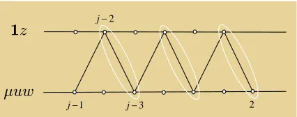
μuw

1z

1

−

j

2

−

j

3

−

j 2

Figure 3: If jis odd, the wordAis of the formz(µuw)(1z)(µuw)(1z)· · ·(µuw)P₁θ1va1_.

from which the two inequalities in (2.26) follow readily. By (2.25), for j>2,

zT_j−1,1

2

∏

Gi

!

Pθ1

1 v

a1_{= z}T

j−1,1 2

∏

n

1

2(1−2i₎12izT_i−1,1+µi,2ui,2wTi−1,2

o !

Pθ1

1 v

a1_{. (2.27)}

If we drop all sub/superscripts and expand the scalar expression above, we find a sum of 2j−2 _words

zaj−1· · ·a2P₁θ1va1, where eachaiis of the formµuwor1z(suitably scaled). By (2.26), however, the only

nonzero word is of the form

A=z(µuw)(1z)(µuw)(1z)· · ·Pθ1

1 v

a1_.

This necessitates distinguishing between even and odd values of j.

Case I.(odd j>2:Figure 3) It follows from (2.26) that

zT_j−1,1

2

∏

Gi

!

=zT_j−1,1µj−1,2uj−1,2wTj−2,2 3

∏

oddi=j−2

n

1

2(1−2i₎12izT_i−1,1µi−1,2ui−1,2wTi−2,2

o

=2µj−1,2wTj−2,2 3

∏

oddi=j−2

n

1

1−2i12iµi−1,2wTi−2,2

o

=αoddj w T

1,2,

where

αoddj =2(−1)(j+1)/2µ2,2 3

∏

oddi=j−2

γiµi+1,2

2i₋₁ . (2.28)

One must verify separately that this also holds for the case j=3, where, by convention, the product

∏i evaluates to 1 because the indices do not go down. Recall that, by (2.9,2.24),w1,2= (1,1)T and kva1_k

2= √

5n−c. ByLemma 2.3and the submultiplicativity of the Frobenius norm,

wT_1,2Qθ₁1va1 ≤

w_1,2

2

Qθ₁1

F

va1

2<e −n1.5_.

By (2.17), it follows that

wT_1,2Pθ1

1 v

a1 _=wT

1,2 12πT+Qθ11

va1 _=va1

1 +v

a1

2 ±O e −n1.5

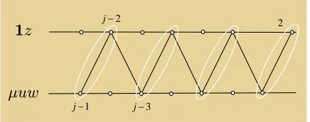
μuw 1z 1 − j 2 − j 3 − j 2

Figure 4: If jis even, the wordAis of the formz(µuw)(1z)(µuw)· · ·(1z)P₁θ1va1_.

and

A=zT_j−1,1

2

∏

Gi

!

Pθ1

1 v

a1 _=αodd

j w T

1,2P θ1

1 v

a1

=αodd_j (va₁1+va₂1)±O αodd_j e−n1.5.

(2.30)

Case II.(even j>2:Figure 4)

zT_j−1,1

2

∏

Gi

!

=zT_j−1,1

3

∏

oddi=j−1

n

µi,2ui,2wTi−1,2 2(1−21i−1₎

1₂i−1zT_i−2,1

o

=zT_j−1,1

3

∏

oddi=j−1

n

1 2(1−2i−1₎

µi,2ui,2γi−1zTi−2,1

o

=βjzT_1,1,

where

βj= (−1)j/2+1

3

∏

oddi=j−1

γi−1µi,2 2i−1₋₁.

It follows that

A=zT_j−1,1

2

∏

Gi

!

Pθ1

1 v

a1₌

βjzT_1,1P₁θ1va1.

By (2.17),

zT_1,1Pθ1

1 v

a1 _=zT

1,1 12πT+Qθ11

va1_=zT

1,1Qθ11v

a1 ₌

µ1,2 va11−v

a1

2

; (2.31)

therefore,

A=αevenj v a1

1 −v

a1

2

, (2.32)

where

αevenj = (−1) j/2+1

µ1,2 3

∏

oddi=j−1

γi−1µi,2

2i−1₋₁. (2.33)

This concludes the case analysis. Next, we still assume that j>2 but we remove all restriction on parity. Recall thatGiis only an approximation ofFi and, instead of (2.27), we must contend with

zT_j−1,1

2

∏

Fi

!

Pθ1

1 v

a1_{= z}T

j−1,1 2

∏

n

1

2(1−2i₎12izT_i−1,1+

2i

∑

µi,kui,kwTi−1,k

o !

Pθ1

1 v

If, again, we look at the expansion of the product as a sum of words

B=zaj−1· · ·a2P₁θ1va1, then we see that eachB-word is the form

z(µuw){1z,µuw}{1z,µuw}{1z,µuw} · · ·P₁θ1va1,

whereµ,u,ware now indexed byk. Recall that previously the only word was of the form A=z(µuw)(1z)(µuw)(1z)· · ·P₁θ1va1.

We show that|A|always dominates|B|.

Lemma 2.4. For any2< j≤logn,

zT_j−1,1

2

∏

Fi

!

Pθ1

1 v

a1₌

(

(1+εn)(va₁1+va₂1)αoddj if j is odd;

(1+ε_n0)(va₁1−va₂1)αeven_j else, whereεn,εn0 are reals of absolute value O(e−n).

Proof. Note that, by (2.26),γi>2i−1−1 for anyi≥1. Also, by (2.9),va₁1+va₂1=n−candv₂a1−va₁1 =

3n−c. It follows from (2.28,2.30,2.32,2.33) that, for any 2< j≤logn,

|A|=

zT_j−1,1

2

∏

Gi

!

Pθ1

1 v

a1

≥ 1

n

c+1 (

|µ2,2µ4,2· · ·µj−1,2| if jis odd; |µ1,2µ3,2· · ·µj−1,2| else.

(2.35)

Let’s extend our notation by defining, fori>1,

  

 

µi,1=1₂(1−2i)−1;

ui,1=12i; wi−1,1=zi−1,1. Then, anyB-word is specified by an index vector(kj−1, . . . ,k2):

Bkj−1,...,k2 =w

T j−1,1

2

∏

µi,kiui,kiw

T i−1,ki

Pθ1

1 v

a1_.

Observe that theA-word we considered earlier is a particularB-word, i. e.,

A=B_{2,1,2,1,. . .}

| {z }

j−2 .

Since we wish to show that all the otherB-words are considerably smaller, we may ignore the settings of

kithat make aB-word vanish. All the conditions on the index vector are summarized here:

  

 

1≤ki≤2i;

kj−16=1 ;

kiki−16=1 (2<i< j).

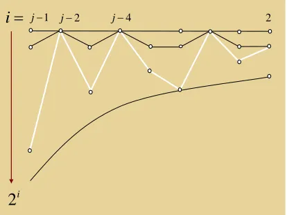
1 −

j j−2 j−4 2

i

2

=

i

Figure 5: The top horizontal line representski=1. The white dots below the line correspond toki=2.

TheB-word in white is brought into canonical form (black jagged line) by setting all the indiceski>2

to 2. This cannot cause the magnitude ofBto drop. We may also assume that the end result is not the

A-word, as this would cause an exponential growth in line with the lemma.

By (2.18, 2.20), for all i>1 and k ≥1, kui,kk2≤2i/2 and for i,k≥1, kwi,kk2≤2i/2+O(1); so, by Cauchy-Schwarz, fori>2 andk,l≥1,

wT_i−1,ku_i−1,l

≤2i+O(1).

Since 2< j≤logn,

w

T

j−1,1uj−1,kj−1

2

∏

wT_i,k i+1ui,ki

<n

2 logn

;

therefore,

B_k

j−1,...,k2

≤n2 logn

2

∏

µi,ki

× wT_1,k

2P

θ1

1 v

a1

. (2.37)

We prove that allB-words are much smaller thanAin absolute value.

Lemma 2.5. All B-words distinct from A satisfy:

Bkj−1,...,k2

<e−n

1.2

|A|.

Proof. SinceP1is stochastic, by (2.9),

wT_1,k

2P

θ1

1 v

a1

=O(kva1k_∞) =O(n−c)<1,

and the upper bound (2.37) becomes

Bkj−1,...,k2

≤n2 logn

2

∏

µi,ki

1 −

j

1 +

a

2

=

i

1 −

a

Figure 6: We trace the index vectors of theAandB-words from left to right until they diverge (i=a). In this case, jis odd and the index vector of theB-word is(2,1,2,1,2,2,1,2,2).

To maximize the right-hand side of (2.38), byLemma 2.3, we may replace any instance ofki>2 by

ki=2 (Figure 5). This does not contradict conditions (2.36) since no index is set to 1. Note the importance

for this step of having all vectorial presence removed in (2.38). We may assume that the newB-word is notA, so its index vector is not of the form(2,1,2,1, . . .). Indeed, if we ended up with this pattern, and hence withA, obviously at least one index replacement would have taken place. ByLemma 2.3, any such replacement would cause an increase by a factor of at leasten1.5 andLemma 2.5would follow. So, we may assume now thatki∈ {1,2}and

(kj−1,kj−2, . . . ,k2)6= (2,1,2,1, . . .).

Scan the string(kj−1, . . . ,k2)against(2,1,2,1, . . .)from left to right and letkabe the first character that

differs (Figure 6). By (2.36),kj−1=2, so 2≤a≤ j−2; hence j>3; since we cannot have consecutive ones,ka=2 and j−ais even. By (2.35,2.38) andLemma 2.3,

|Bkj−1,...,k2|

|A| ≤(n

c+1_n2 logn

)|µj−1,2µj−2,1µj−3,2· · ·µa+1,2µa,2µa−1,ka−1· · ·µ2,k2|

|µj−1,2µj−3,2· · ·µa+1,2µa−1,2µa−3,2· · · |

≤n3 logn|µj−2,1µj−4,1· · ·µa+2,1µa,2µa−1,ka−1· · ·µ2,k2|

|µa−1,2µa−3,2· · · |

.

The first numerator mirrors the index vector of theB-word accurately. For the denominator, however, we use the lower bound of (2.35). The reason we can afford such a loose estimate is the presence of the factorµa,2, which plays the central role in the calculation by drowning out all the other differences. Here are the details. All the coefficientsµ are less than 1 and, byLemma 2.3,|µa−1,2| ≤ |µa−l,2|; therefore,

|Bkj−1,...,k2|

|A| ≤n

3 logn |µa,2| |µ_alog₋₁n_,2|

<n3 logn |µa,2|

|µ_an_−1,2|<n

3 logn

e−n1.5.

which provesLemma 2.5.

There are fewer thannlognB-words; so, byLemma 2.5, their total contribution amounts to at most a fractionnlogne−n1.2 of|A|. In other words, by (2.34), for j>2,

zT_j−1,1

2

∏

Fi

!

Pθ1

1 v

a1 _{= (1±O(e}−n_))zT

j−1,1 2

∏

Gi

!

Pθ1

1 v

2/3 2/3

1/3 1/3

1/3 1/3

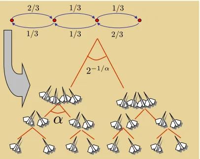
α

2−1/α

Figure 7: Birds join in flocks of size 2, 4, 8, etc., each time flying in a direction closer to theY-axis. The angle decreases exponentially at each level. The big arrow indicates the Markov chain corresponding to a four-bird flock.

and the proof ofLemma 2.4follows from (2.9,2.30,2.32).

Recall from (2.16) that, for j>1,

maj =

1 2(1−2j₎z

T j−1,1

2

∏

Fi

!

Pθ1

1 v

a1_.

We know from (2.26,2.28,2.33) that neitherαeven_j norαodd_j is null. ByLemma 2.4, it then follows that

the first Fourier coefficientmaj never vanishes for j>2. By (2.9), this is also the case for j=1,2, so the

proof ofTheorem 2.1is complete.

3

A lower bound on the flocking time

Theorem 2.1sets the grounds for a lower bound of 2logcn(for constantc) on the convergence time of a flock of birds. The idea is to lift the previous construction to higher dimension and interpret railroad cars as birds and trains as flocks. While checking that the convergence time matches the characteristic time of the corresponding consensus system is easy, to verify the integrity of the flocks takes some effort.

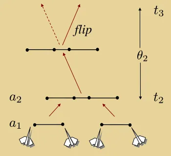
Then birds all start from the X-axis and fly in the(X,Y)-plane, merging in twos, fours, eights, etc., in a pattern mirroring the treeTof the previous section (Figure 7). The horizontal motion slows down drastically as time goes on, which creates a flocking time of 2Θ(logn). The upper bound in [2] tolerates a small amount of noise in the model, which we can use to simplify our construction: specifically, any given flock is allowed a singlevelocityflip, meaning that the vectorvaassociated with nodeabecomes−va_{. The stochastic matrix used for flocking (1.1) is of the formP}

j, as defined in (2.2),

flocking network. Letx(t)denote the vector(x1(t), . . . ,xn(t))of bird positions from left to right, and

writev(t) =x(t)−x(t−1).

x(0) =0,2/3,2,8/3, . . . ,2l,2l+2/3, . . . ,n−2,n−4/3

T

.

Lett1=0 andtj=tj−1+θj−1, for j>1. The velocity vector satisfiesv(t1) =va1 as set in (2.9) and

v(1) =P1va1; in general, fort>0,

x(t) =x(0) +

t−1

∑

P₁sv(1),

hence

x1(t)

x2(t)

=

x1(0)

x2(0)

+

t−1

∑

P₁s(P1va1) = 2 3

0 1

+

t−1

∑

P₁s

n−c

0

.

DiagonalizingP1shows that, for any integers>0,

P₁s=1

2

1 1

1 1+1

2(−3) −s

1 −1

1 −1

.

It follows that, for 0=t₁<t≤t₂,

(

x1(t) =₂tn−c+₂1n−c∑ts−1=0(−3) −s₌1

2n

−c_(t+3 4+

1 4(−3)

1−t_);

x₂(t) =2₃+₂tn−c−1 2n

−c

∑ts−1=0(−3) −s₌2

3+ 1 2n

−c_(t−3 4−

1 4(−3)

1−t_). (3.1)

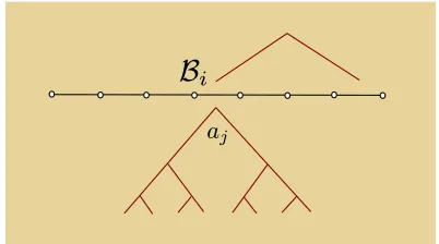
LetBidenote the bird associated with thei-th leaf ofT. Note thatB1always stays to the left ofB2and their distance is

x2(t)−x1(t) = 2 3−

3 4n

−c

1−

−1 3

t

. (3.2)

Left to their own devices, the two birds would slide to the right at speedma1, plus or minus an exponentially

vanishing term; their distance would oscillate around 2/3−(3/4)n−cand converge exponentially fast, with the oscillation created by the negative eigenvalue. This is what happens until the flock ata1begins to interact with its “sibling” flock to the right,(B3,B4). The latter’s velocity vector is(−n−c,0)T at time

t=1 and, fort₁<t≤t₂,

(

x3(t) =2−1₂n−c(t+3₄+1₄(−3)1−t);

x4(t) = 8₃−1₂n−c(t−3₄−1₄(−3)1−t).

(3.3)

The stationary velocity of (B3,B4) is −ma1 =−(1/2)n

−c_{, but the flock is not the mirror image of}

(B1,B2), a situation that would destroy the lower bound construction. In particular, note that the diameter of the flock is

x4(t)−x3(t) = 2 3+

3 4n

−c

1−

−1 3

t

, (3.4)

t

a

a

t

θ

flip

Figure 8: A four-bird flock flipping at timet2+nf.

at distancex₃(t)−x₂(t) =4/3−tn−c. (The linearity intis due to an accidental cancellation that will not occur for bigger flocks.) This implies thatt2=t1+θ1=d(1/3)nce. The two flocks link up at timet2, and

1−n−c<x3(t2)−x2(t2)≤1. (3.5)

Two issues arise: which way does the four-bird flock move and does it stay in one piece? Indeed, if the distance betweenB2andB3is too close to 1, can’t it jump back up above 1 to cause the breakup of the flock? The issue of flock integrity deserves a separate treatment but, in this simple case, we easily verify it. We begin with the motion of the four-bird flock. At timet₂, the flock ata₂is formed with the initial velocity

va2 ₌

Pt2−t1

1 v

a1

−Pt2−t1

1 v

a1

=



    

Pθ1

1

−n−c

2n−c

−Pθ1

1

−n−c

2n−c



    

=1

2n −c



  

1+ (−3)1−θ1

1−(−3)1−θ1

−1−(−3)1−θ1

−1+ (−3)1−θ1



  

. (3.6)

By (2.4), the stationary velocity for the four-bird flock is

ma2=

1 3(

1 2,1,1,

1 2)v

a2₌₋1

2n

−c₍₋₃₎−dnc/3e_.

ByLemma 2.4, for j>2,

maj =

1 2(1−2j₎

(

(1+εn)(va₁1+va₂1)αoddj if jis odd;

(1+εn0)(v a1

1 −v

a1

2 )αevenj else.

(3.7)

It is imperative thatmaj >0. If it is negative, therefore, we must flip the velocity ataj instead of its

We amend the flipping rule so that the left (resp. right) sibling flips if the flocks move left (resp. right) so as to set up a head-on collision. (We refer the reader to [2] for a detailed explanation of why flipping conforms the noisy flocking model with the matching upper bound.)

We now turn to the issue of flock integrity. Instead of negating one of the siblings’ velocity vector at timetj, we wait an extranf steps, for some large enough constant f: the goal is to give the flock enough

time to stabilize so it does not break apart because of the flip. By straightforward diagonalization, we find that, for any integers>0,

P₂s=1

6     1 1 1 1    

(1,2,2,1) +1

6 2 3 s     2 1 −1 −2    

(1,1,−1,−1) +1

6(−3) −s     1 −1 1 −1    

(1,−2,2,−1); (3.8)

therefore, it follows fromx(t) =x(t2) +∑st−=t02−1P

s+1 2 v

a2 _{that, by (3.6),}



 

x1(t) .. .

x4(t)

  =   

x1(t2) .. .

x4(t2)





+ma2(t−t2)

    1 1 1 1     +1 8n −c     11 5 −5 −11    

+n−c

2

3

t−t2+1     −2 −1 1 2     + 1 24n −c₍₋

3)t2−t

    −1 1 −1 1     . (3.9)

It follows from (3.2,3.4) that, fort>t₂, bothx₂(t)−x₁(t)andx₄(t)−x₃(t)are 2/3±O(n−c); therefore, the two end edges of the four-bird flock aresafe, which we define as being of length less than 1 (so as to belong to the flocking network) but greater than 1/2 (so as to avoid edges joining nonconsecutive birds). The middle edge betweenB2andB3is more problematic. Its length is

x3(t)−x2(t) =x3(t2)−x2(t2)− 1 12n

−c ₁₅₋₁₆

2 3

t−t2

+ (−3)t2−t

!

.

We can verify that

15−16

2 3

t−t2

+ (−3)t2−t _≥0,

for allt>t₂, which, by (3.5), shows that the distance between the two middle birds stays is 1−Θ(n−c), which is also 1− |ma1|. This points to a general principle crucial to the integrity of the flocks: when

velocity, so changing their signs cannot jeopardize edge safety. We flesh out the details in the next lemma,

which concludes the lower bound proof.

Lemma 3.1. Any two adjacent birds within the same flock lie at a distance between0.58and1. This holds over the entire lifetime of the flock, whether it flips or not.

Proof. For notational convenience, put ma0 = (1/4)n

−5 _{and define h(i) as the height of the nearest} common ancestor of the two leaves associated with birdsBiandBi+1; e. g.,h(1) =1 andh(2) =2. We prove by induction on jthat, for any 1≤ j<logn,tj≤t≤tj+1, and 1≤i<2j,

1−5₃(n5+jn4)ma_h(i)−1

≤DISTt(Bi,Bi+1)

≤

(

1 ifi=2j−1_andt=t

j;

1−1₄(1−_nj)ma_h(i)−1

else.

(3.10)

Recall thata₀,a₁, etc., constitute the left spine of the merge treeT. By (2.14), the upper and lower bounds above fall between 0.58 and 1, so satisfying them implies the integrity of the flocks along the spine: indeed, the upper bound ensures the existence of the desired edges, while the lower bound, being greater than 1/2, rules out edges between nonconsecutive birds. Before we proceed with the proof, we should explain why the upper bound of (3.10) distinguishes between two cases. In general, once two consecutive birds are joined in a flock, they stay forever at a distance strictly less than 1. There is only one exception to this rule: at the timetwhen they join, the only assurance we can give is that their distance does not exceed 1; it could actually be equal to 1, hence the difficulty of a nontrivial upper bound whent=tjand

i=2j−1.

Relations (3.10) show that the timeθjbetween the formation of the flock atajand its next collision

ataj+1is proportional to the reciprocal of the stationary velocity|maj|; note that choosingclarge enough

makes the delaynf inconsequential. This implies that the earlier setting ofθj in (2.5) must now be

understood up to a constant factor, i. e., asθj=Θ(|m−1aj |); the previous analysis still holds. For the case j=1, we observe that, for 0≤t≤t₂, by (3.2,3.4),

2 3−n

−c_≤x

2(t)−x1(t)≤x4(t)−x3(t)≤ 2 3+n

−c_.

Assume now that j≥2. By applying successively (2.8,2.11,2.14), we find that

Q

θj−1

j−1v

aj−1

2≤2 2j−1

e−Ω(θj−141−j)_kvaj−1_k

2≤e−Ω(n −2_/|m

a j−1|)

≤e−2n−Ω(n−2/|ma j−1|)_<m

aj−1

e−2n.

By (2.10),

vaj _=± P

θj−1

j−1 vaj−1 −P_jθ₋₁j−1vaj−1

!

=maj−1

1 −1

⊗1₂j−1±

Qθj−1

j−1vaj−1 −Qθ_j−1j−1vaj−1

!

.

drifts to the right while its sibling, with the higher-indexed birds, flies to the left; hence the certainty that, after flipping, the “fixed” part of the velocity vectorvaj _{is of the form|m}

aj−1|(1,−1)

T_⊗1

2j−1. (In fact, to

achieve this is the sole purpose of flipping.) It follows that

vaj ₌

m_aj−1

1 −1

⊗1₂j−1+ζ, with kζk2<

m_aj−1

e−n. (3.11)

For 1≤i<2j, define

χi= ( i

z }| {

0, . . . ,0,−1,1,0, . . . ,0

| {z }

2j

)T.

By (2.7), fors≥1,

χiTP s jv

aj_=m

ajχ

T

i 12j+χiTQ s jv

aj ₌ χiTQ

s jv

aj_;

hence, fortj<t≤tj+1,

DISTt(Bi,Bi+1) =DISTtj(Bi,Bi+1) +

t−tj

∑

(−1)f(s)χiTQsjvaj, (3.12)

where f(s) =1 if there is a flip ands>nf, and f(s) =0 otherwise. Note that there is no risk in using DISTt(Bi,Bi+1), instead of the signed version,xi+1(t)−xi(t), that birds might cross unnoticed: indeed,

the bound in (2.11) applies to all the velocities, so that distances cannot change by more thanO(n1−c)

in one step. This implies that a change of sign forxi+1(t)−xi(t) would be preceded by the drop of

DISTt(Bi,Bi+1)below 1/2 and a violation of (3.10). By Cauchy-Schwarz and (2.8,3.11),

|χiTQ s

jζ| ≤

√

2kQs_jζk2≤ √

2 22j+1e−Ω(s4−j)kζk2≤O(n2)e−n−Ω(s/n

2₎ maj−1

;

and, sincenis assumed large enough, fors≥1,

χ_iTQs_jζ

<e−

1 2n−sn

−3 maj−1

. (3.13)

Likewise,

χ_iTQs_jvaj ≤

√

2Qs_jvaj

2≤n

1.45_e−Ω(s/n2) vaj

2

≤n1.45e−Ω(s/n2) m_a

j−1

√

n+ζ

2

.

Fors≥1 and 1≤i<2j, by (3.11),

χ_iTQs_jvaj ≤n2

maj−1

e−Ω(s/n

2₎

. (3.14)

Recall that j≥2. To prove (3.10), we distinguish between two cases: whether the birdsBi,Bi+1are joined at nodeaj or earlier.

Case I.(i=2j−1): The edge(i,i+1)is created at nodeajandh(i) = j, where 2≤ j<logn(Figure 9).

B

aj

Figure 9: The birdsBiandBi+1are joined together at timetj.

lower bound, we observe that at timetj−1 the two middle birds were more than one unit of distance

apart. By the expression of the velocity given in (3.11), which expresses the displacement right beforetj,

neither bird moved by more than(1+e−n)|maj−1|in that one step; therefore,

DISTtj(Bi,Bi+1)>1−3

maj−1

, (3.15)

which exceeds the lower bound of (3.10), i. e.,

1−5 3(n

5_+jn4_)|m

ah(i)−1|.

Assume now thattj<t≤tj+1. Observe that

1₂j(

2j

z }| {

1

2,1, . . . ,1, 1 2)

n ₁

−1

⊗1₂j−1

o

=0.

Thei-th row ofPjis the same as the(2j+1−i)-th row read backwards. This type of symmetry is closed

under multiplication, so it is also true ofPs_j. By (2.7), for anys≥0, it then follows that

Qs_jn

1 −1

⊗1₂j−1

o

=Ps_jn

1 −1

⊗1₂j−1

o

=b(₁s), . . . ,b(s)

2j−1,−b (s)

2j−1, . . . ,−b (s)

1

T

.

The following recurrence relation holds:b(_i0)=1; fors≥0, we get the identities below forl≤2j−1, plus an antisymmetric set forl>2j−1:

b(_ls+1)= 1

3

          

         

b(₁s)+2b(₂s) ifl=1;

b_l(₋₁s) +b(_ls)+b_l(₊s)₁ if 1<l<2j−1;

b(s)

2j−1₋₁ ifl=2

j−1_;

−b(s)

2j−1₋₁ ifl=2

j−1_+1;

−b(₂sj)_+2−l−b (s)

2j_+1−l−b (s)

2j_−l if 2

j−1_+1<l<2j_;

We find by induction that

b(₁s)≥ · · · ≥b(s)

2j−1 ≥3

−s

;

therefore,

χ₂Tj−1Q

s j

n ₁

−1

⊗1₂j−1

o

=−2b(₂sj)−1 <−3

−s

. (3.16)

Considering that the two middle birds in the flock foraj get attached in the flocking network at timetj,

DISTtj(Bi,Bi+1)≤1. Assume that the flock atajdoes not undergo a flip. Then, by (3.11,3.12,3.13), for tj<t≤tj+1,

DISTt(Bi,Bi+1)≤1+

t−tj

∑

χiTQ s

jv aj

≤1+maj−1

t−tj

∑

χ₂Tj−1Qs_j

n 1

−1

⊗1₂j−1

o

+

t−tj

∑

χ₂Tj−1Qs_jζ

≤1−1 3

m_a

j−1

+

∑

s≥1

|χ₂Tj−1Q

s jζ|

≤1−1 3

m_a

j−1

+

m_a

j−1

∑

s≥1

e−12n−sn

−3

<1−1

3(1−o(1))

m_aj−1

=1−

1

3(1−o(1))

m_a

h(i)−1

,

which proves the upper bound in (3.10) fori=2j−1. The negative geometric series we obtain from (3.16) reflects the “inertia” of the two flocks as they collide and penetrate each other’s zone of influence before being stabilized. Suppose now that the flock ataj undergoes a flip at timetj+nf. The previous analysis

holds fortj<t≤tj+nf; so assume thattj+nf <t≤tj+1. By (3.14) andh(i) = j,

t−tj−nf

∑

χ_iTQs+n

f

j v

aj

≤

t−tj−nf

∑

n2ma_h(i)−1

e−Ω(sn

−2_+nf−2₎

=o ma_h(i)−1

.

By (3.12), therefore,

DISTt(Bi,Bi+1) =DISTtj(Bi,Bi+1) +

nf

∑

χiTQsjvaj− t−tj

∑

χiTQsjvaj

≤DIST_t

j+nf(Bi,Bi+1) +

t−tj−nf

∑

χ_iTQs+n

f

j v

aj

<1−1

3(1−o(1))

mah(i)−1

+o

mah(i)−1

<1−1 4

mah(i)−1

.