(UDC: 004.032.26:535.333)
Growing Cell Structures Neural Networks for Designing Spectral Indexes
S. Delgado1, C. Gonzalo2, E. Martínez2, Á. Arquero2
1Department of Organization and Structure of Information, Universidad Politécnica de Madrid
Ctra. Valencia, Km. 7, 28031 Madrid, Spain e-mail: [email protected]
2Department of Architecture and Technology of Computer Systems, Universidad Politécnica de Madrid. Campus de Montegancedo, 28660 Madrid, Spain
e-mail:{chelo, emartinez, aarquero}@fi.upm.es
Abstract
Remote sensing can be defined as the technique that facilitates the acquisition of land surface data without contact with the material object of observation. The development of tools for analyzing and processing multispectral images captured by sensors aboard satellites has provided the automation of tasks that could not be possible otherwise. The main problem related with this discipline is the large volume of data of multidimensional nature that must be handled. The concept of spectral index emerged as an idea to reduce the number of dimensions to one, and thus facilitate the study of different features associated to the types of land cover categories that exhibits a multispectral image. Formally, a spectral index is defined as a combination of spectral bands whose function is to enhance the contribution of one type of land cover mitigating the rest of covers. In this work a no-supervised methodology to analyze and discover spectral indexes based on growing self-organizing neural network (GCS-Growing Cell Structures) is presented.
Keywords: spectral index, self-organizing map, growing cell structures, topographic map, component planes.
1. Introduction
Address current issues like precision agriculture, quality water estimation or evaluation of damages caused by natural disasters need to deal with information remotely captured by sensors on board satellites. Spectral sensors allow registering data from large Earth surface areas within different parts of the electromagnetic spectrum, ranging from the visible light through the infrared and ending in the microwaves. This makes necessary to work with large multispectral satellite imageries formed by a great volume of pixels, with several radiometric measures (spectral bands) associated to each point. The process of extracting useful information from multispectral images to a reasonable cost makes the development of tools and techniques of data exploitation necessary.
specific characteristics, masking the rest. Many spectral indexes have been proposed in the literature to detect different features of the images remotely detected. One of the most widely used is NDVI (Normalized Difference Vegetation Index), developed by Rouse et al. (1973). Some of the applications in which this index has been applied are for estimating leaf water content and other physiological variables for grasses (Tucker 1979), for deriving fuel moisture content (FMC) for Mediterranean grasslands and shrub species (Chuvieco et al. 2004), or for vegetation water content estimation (Jackson et al. 2004). Several alternatives of vegetation indexes for very specific applications and remote sensors have been proposed too, such as GEMI (Global Environment Monitoring Index) proposed in (Pinty & Verstraete 1992) and exploited in (Verstraete & Pynti 1996), GVMI (Global Vegetation Moisture Index) to study the vegetation water content (Ceccato et al. 1996), or SAVI (Soil Adjusted Vegetation Index) based on a NDVI modification to make it less dependent on variations of soil properties, for partial vegetation cover (Huete 1988). Water is another one of the terrestrial covers for which some spectral indexes have been developed. The best known is NDWI (Normalized Difference Water Index) (McFeeters 1996) proposed primarily to delineate water bodies and enhance its presence in remotely sensed imagery, while simultaneously eliminating soil and vegetation features. When remote sensors offer a good spectral definition, in particular the medium infrared, MNDWI (Modified Normalized Difference Water Index) can be used (Hui et al. 2008), that usually provides better results in the discrimination of water cover that the previous one. Although urban areas are a small fraction of the Earth’s surface, there are many satellite images including this type of covers, making very interesting having spectral indexes capable to discriminate them. When the spectral definition of the sensors includes near and medium infrared, NDBI (Normalized Difference Build-up Index) (Zha et al. 2003)(He & Xie 2008) can be used.
The spectral (number of bands) and spatial (meters squared by pixel) definition of the remote sensors are two relevant aspects that strongly affects the type of spectral indexes that can be applied to the images captured by them. Higher spatial resolution assures better homogeneity of land covers within pixels (i.e., no mixtures), but a large spatial variability. On the other hand, higher spectral resolution gives more chances of finding specific spectral indexes. The specific characteristics of land covers present in the remotely registered geographical area, like the season of the year, the climatic conditions, etc, are other factors that also affect the type of spectral indexes that can be applied to images. All this peculiarities make necessary the development of tools that facilitate the design and validation of optimal spectral indexes for the specific characteristics of sensors and land covers which will be treated.
This paper proposes a graphical tool based on self-organizing neural networks, for studying the viability of using different spectral indexes for specific spectral images captured by particular remote sensing instruments. Specifically, the self-organizing model used is the Growing Cell Structures (GCS) (Fritzke 1994). An image registered by the ETM+ sensor (Landsat 7) has been used to illustrate the proposed graphical technique to validate spectral indexes. It has been analyzed the most representative spectral indexes for vegetation, water, and soil covers.
The rest of the paper is organized as follows: section 2 introduces the growing cell structures methodology, section 3 presents the experiments and finally, conclusions are included in section 4.
2. Growing Cell Structures
map can be used for several tasks of pattern preprocessing, e.g. for subsequent classification, or if the network has an output layer consisting of neurons arranged in a two-dimensional structure, to project and to visualize high dimensional signals in a two-dimensional space. Even though the first model of SOM proposed by Kohonen is a powerful tool that has been widely used in the field of exploratory data analysis, this network has associated several undesirable features. One of the most relevant is the static network architecture, that forces setting the complete topology before the training phase, and it is not possible to change it back later. This feature requires a good knowledge of the input space, to be able to establish an architecture that fits well, and thus to obtain a network with a good topology preserving grade. The network training process tries to find a simplified model of the input space, as well as the projection of multidimensional input space in the two-dimensional output layer, that will maintain the existing relations of the input patterns. Informally, the term topology preservation measures the quality of this simplified model. Not always it is possible to know well enough the input data space to set up a SOM network, and in some cases even knowing it, it is not possible to establish an architecture of a Kohonen network that well adapts to the input data model. When input data space has a high dimensional nature it is difficult to know the characteristics present in the space of signals. On the other hand, in many cases the input space is formed by signals that are distributed in isolated clusters separated by areas with low or null probability density. In these cases, the Kohonen’s model is not a good election. In 1994, B. Fritzke proposed a dynamic SOM network model called Growing Cell Structures (GCS), to address the limitations of the Kohonen’s SOM. Although GCS model exhibits very good characteristics, it has a weakness associated with the interpretation and the adjustment of some of the training parameters, in particular with those related to the removal of neurons. Therefore, in this work we have used the modification of the GCS training algorithm that we introduce in (Delgado et al. 2004). In the rest of this section, diverse aspects related to the GCS network model and the training algorithm used for this study are exposed.
2.1 GCS architecture
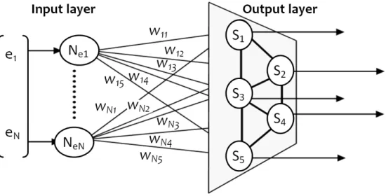
GCS network has an architecture consisting of an input layer containing so many units as dimensions have the input patterns and one output layer formed by several neurons. All the input units are connected with all the output ones through feed forward connections that have associated a weight. In addition, the units of the output layer are connected between them by neighborhood links, forming a topology of k-dimensional hyper tetrahedrons. For k=1 the basic neighborhood connection topology is a line segment connecting 2 units, for k=2 a triangle connecting 3 units, and for k=3 and higher is a tetrahedron or a hyper-tetrahedron connecting k+1 units. In order to use GCS networks to generate a two-dimensional map that facilitates the projection and visualization of high dimensional input signal in a two-dimensional space, a factor of k=2 has been used in all the experiments, so the neighbor connections exhibit structures formed by groups of triangles (Fig. 1).
Each time a new input pattern e = (e1, …, en) is presented to the network, each one of the
input units transmit a component, ei, to each one of the output neurons. On the other hand, each
output neuron c compute the Euclidean distance between the pattern and its synaptic vector wc
= (w1c,…, wnc). GCS network is based on the model of the winner takes it all, reason why only
one output neuron, bmu (best matching unit), is activated whenever a pattern is presented to the network, which will be that one with the synaptic vector more similar to the input pattern:
arg min
bmu c
S
e w
(1)vector wi. In this way, the set of all the synaptic vectors of the network represents a simplified
model of the input signal space.
At this point it is possible to give a formal definition of the topology preserving measurement in a GCS network. When all the similar input patterns are mapped by neighboring output neurons and all the neighboring output neurons respond to similar input patterns, it can be said the GCS network is perfectly topology preserving, which indicates the goodness of the simplified model that the network represents. This is a very important characteristic when the two-dimensional output layer is used to generate graphs to analyze the input signal space, as it is described in the following sections.
Fig. 1. GCS architecture
2.2 GCS adaptation process
To obtain a GCS network that can be used as simplified model of a particular space of input signals is necessary to train the network through a learning phase. During this process, a set of training patterns are presented iteratively to the network and the synaptic vectors of the output neurons are adapted, looking for that each unit represents a group of similar input patterns. At the beginning of the training phase, a GCS network consists of three interconnected neurons (a basic k-dimensional structure, with k=2). On each adaptation step a new pattern is processed by the network, the bmu is calculated, and its synaptic vector and the synaptic vectors of its neighboring units are modified according to equations 2 and 3 (where εb > εn), respectively.
bmu b bmu
w
e w
(2)
neighbor of
c n c
w
e w c bmu (3)
units in such a way that the expected value of a certain error measure becomes equal for all the output neurons (i.e., the sum of the Euclidean distances between the synaptic vector of the neuron and all the patterns for which is the bmu).
Periodically superfluous neurons are removed of the output layer of the network in order to achieve better topology preserving grades when the input signal space consists of several separated regions with positive probability density. The objective is to remove those neurons whose synaptic vectors are located in areas of the input space with low or null presence of patterns. During the removal procedure, some neighborhood connections are also destroyed ensuring that the output layer maintains the topology of triangular groups of neighboring neurons, although the neighborhood output mesh can result broken in two or more sub-meshes. All the details about the modifications of the GCS training algorithm that has been used in this work can be found in (Delgado et al 2004).
2.3 GCS topographic map
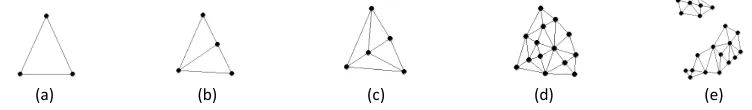
In a trained GCS network, the output layer is a map that exhibits the relations of the training patterns. When the neighborhood architecture of a GCS network is determined by a k=2 factor, the output layer is formed by one or more two-dimensional meshes that connect neurons by triangular neighborhood connections. If the GCS network exhibits a good degree of topology preserving, the output layer will hold relevant information about training patterns relations, so it would be very interesting to be able to generate a projection of this layer in a bi-dimensional plane and consequently have a graph to display this knowledge. This feature is really relevant when the input space has a high-dimensional nature that makes difficult its analysis. This graph is known as the topographic map and is formed by the neurons and the neighborhood connections of the output layer projected over the plane. The coordinates in which each neuron is shown in the topographic map are calculated during the training process, as detailed in (Delgado et al. 2007). Fig. 2 shows different phases of the evolution of the coordinates of the neurons in the topographic map during the training process of a GCS network. When the GCS output mesh results broken in two or more sub-meshes as consequence of the removal of neurons (Fig. 2e), the topographic map shows this characteristic without needing additional information, reason why it offers an immediate visualization of clusters of the input signal space.
Fig. 2. Topographic map evolution during a GCS training process.
The GCS network topographic map can be enriched including information stored by the network. In this way, several graphs can be generated to visualize different characteristics of the high-dimensional input space (Delgado et al. 2007). Two of the most widely used maps are the distances map and U-matrix. In the first, a value is assigned to each neuron, calculated as the mean value of the Euclidean distances between the synaptic vector of the unit and the synaptic vectors of all its neighbor units. With this information, a gray level within a scale delimited by the maximum and minimum value for all the neurons is assigned to the unit. U-map represents the same information than distances map but, in addition it includes the distance between all the neighboring neurons (painted in a circle shape between each pair of neighbor units). Both maps are often used for the analysis of clusters, where areas in dark tones identify clusters and zones
in clear tones discover boundaries between them. Another map that turns out useful to clusters analysis is the direct visualization, where each neuron is drawn like a big square that contains the synaptic vector in graphical format (spectral signature). When GCS network is trained with removal of neurons, these three graphs can be used to validate the correct formation of clusters.
Fig. 7 and 8 show two examples of U-matrix and direct visualization maps of two GCS trained networks.
2.4 GCS component planes
The simplified model of the input data that the GCS network represents is stored in the synaptic vectors of the output neurons, which have the same dimension that the input patterns. The first component of all synaptic vectors maintains the information of the first dimension of the input space, the second component about the second dimension, etc. The isolated analysis of each input space dimension can be performed using the maps of component planes. So many topographic maps are generated as dimensions have the synaptic vectors, and each one includes information about one component only. For example, in the first component plane each neuron has assigned the value of its first synaptic vector component. Using a scale delimited by the maximum and minimum value for all the neurons, a gray level is assigned to each unit. When all the component planes are generated, relations between weights can be appreciated if similar structures appear in identical places of two different component planes. Fig. 7 and 8 show the component planes of two GCS trained networks.
2.5 GCS combined component planes
This paper proposes a new gray scale topographic map for analyzing spectral indexes that can discriminate different types of land cover categories: the combined component plane. This map is generated using a specific combination of components. For example, (w4-w3)/(w4+w3)
generates a topographic map in which each neuron has assigned the gray level associated to the value calculated subtracting the component 4 from component 3 of its synaptic vector and dividing by their addition. Clear zones in the combined component plane will identify neurons with high values of the spectral index, i.e., neurons sensitive to the spectral index. If the combined component plane of a GCS network with several isolated clusters in the output layer shows one or more clusters with all its units in a clear tone and the rest of clusters in dark tones (low values for the spectral index), this will be a good indicator of the discrimination capacity of the spectral index.
3. Experiments and discussion
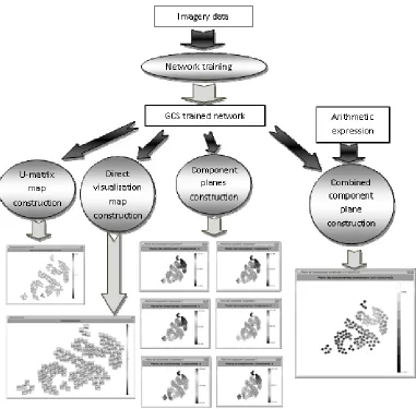
several combined component planes from the arithmetic expressions established by the operator.
Fig. 3. Computational scheme of the software tool developed.
Some experiments have been carried out using this software tool. They are exposed in the remainder of this section.
3.1 Data
correspond with Blue, Green, and Red visible spectrum, and with Near Infra Red (NIR), Mid-Low-IR, and Mid-Hig-IR, respectively.
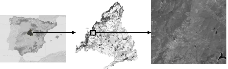
A whole of 1500 representative pixels of the six land cover categories of this scene have been carefully selected and labeled in order to compare them with the results obtained with the GCS simplified model. Fig. 5 shows the mean values of each land cover calculated from these data.
Fig. 4. Study area located in Spain.
Fig. 5. Spectral signatures mean values for the six land cover categories.
3.2 Methodology
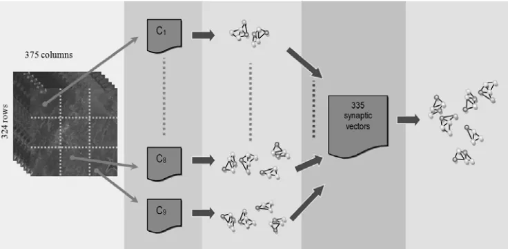
The original image of 324 rows by 375 columns of pixels has been divided in 9 areas with the same size of 13500 pixels (Fig. 6). The original volume of information is too high to train a single GCS network that represents a good simplified model of the input data. With each one of the 9 areas a GCS network with removal of neurons has been trained, ending when a stable number of clusters is fulfilled. LUPD insertion criterion has been used in all the networks, getting a GCS simplified model with the same probability distribution that the input space. Table 1 shows the number of clusters and the number of neurons that contains each of these 9 networks.
Considering that the collection of all synaptic vectors of the 9 networks provides a simplified model of the 121500 pixels of the original image, a new data set with the information of the 335 synaptic vectors has been generated. With this group, two new GCS networks have been trained with removal of units, the first using LEAE insertion criterion and the second with LUPD, and finalizing the training phase when at least 6 isolated clusters of neurons appear in the output layer. The network trained with LEAE finally has 133 neurons and using LUPD 78, both with 6 isolated clusters in the output layer. Fig. 7 and 8 show the mean value of the synaptic vectors by cluster, the U-matrix, the direct visualization map and the component planes associated to both GCS networks.
Fig. 6. Methodology phases. From left to right: original image divided in 9 cuts. Each cut has 13500 pixels, and is used to train a GCS network. The 335 synaptic vectors are joined and used
to train a final GCS network with 6 clusters.
Area Number of clusters Number of neurons
C1 2 40
C2 5 35
C3 3 40
C4 3 37
C5 4 29
C6 4 40
C7 4 34
C8 4 42
C9 4 38
Table 1. Number of clusters and neurons obtained in the 9 GCS networks.
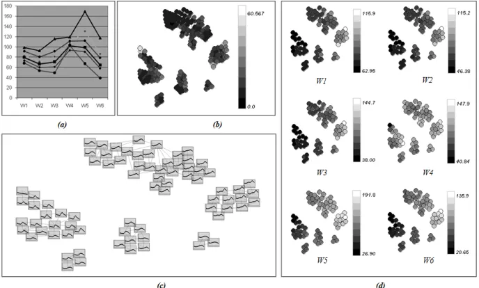
Fig. 7. (a) Synaptic vectors mean values calculated for the six cluster of the GCS network trained with LEAE. (b) U-matrix. (c) Direct visualization map. (d) Component planes.
Fig. 8. (a) Synaptic vectors mean values calculated for the six cluster of the GCS network trained with LUPD. (b) U-matrix, (c) direct visualization map, and (d) component planes of this
3.3 Spectral indexes
This section outlines some of the combined components maps that have been applied to the GCS network trained with LEAE criterion. In particular, the spectral indexes NDVI to discriminate vegetation, NDWI and MNDWI for water and, finally NDBI for soil covers have been explored.
The formal definition of NDVI (Normalized Difference Vegetation Index) is:
NDVI
nir rednir red
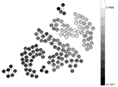
(4)This index exploits the fact that the vegetation covers absorb very well solar radiation in the visible band (due to the presence of chlorophyll and other absorbing pigments in the leaves) and strongly scatters solar radiation in the near-infrared band. Most other natural surfaces present a rather different spectral behavior. This spectral index takes values in the rank [- 1, 1], and takes relatively high values (0.3 to 0.6) on vegetation land covers. When a LANDSAT image is employed, bands TM4+ (NIR) and TM3+ (visible Red) are used to calculate the NDVI. Fig. 9 shows the combined component plane of the GCS network using the NDVI. It can be seen that there is only one cluster of neurons that clearly identifies the vegetation land cover (the only one with clear colors).
Fig. 9. Combined component planes using NDVI.
NDWI (Normalized Difference Water Index) and MNDWI (Modified Normalized Difference Water Index) indexes can discriminate water surfaces. The definition of both is given by equations 5 and 6 respectively.
NDWI
green nir green nir
(5)MNDWI
green mirgreen mir
(6)NDWI index make use of TM2+ (visible Green) and TM4+ (NIR) bands, and MNDWI TM2+ and TM5+ (Mid-IR). Fig. 10 includes the combined component plane of the GCS network using NDWI and MNDWI. Clearly, MNDWI index makes better discrimination of the water cover that NDWI. In this case, as in the NDVI index, there is only one cluster of neurons that clearly identifies the water cover.
Fig. 10. Combined component planes using NDWI (left) and MNDWI (right).
Finally, NDBI index can be used to discriminate soil covers:
NDBI
mir nirmir nir
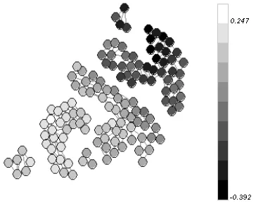
(7)The NDBI (Normalized Difference Build-up Index) index combines the Mid-IR and Near-IR spectra, i.e. the TM4+ and TM5+ bands of the LANDSAT satellite, respectively. Fig. 11 includes the combined component plane of the GCS network using NDBI. There are three clusters that identify different types of soil coverings (those with clear tones). The intermediate cluster that appears between the three soil clusters and the vegetation one characterizes a mixed cover of soil and vegetation.
Fig. 11. Combined component planes using NDBI.
3.4 Image processing
Making use of the spectral indexes, the GCS network can be used as a mask to discriminate different types of land covers present in the image. In order to do it, when a valid spectral index with the capacity to discriminate a specific land cover is identified using the GCS combined component plane, all the neurons within the clusters that clearly identifies that index are labeled with the name of the land cover. Only those clusters of neurons in which all the units identify the same land cover discriminated by the index are labeled. This labeling process can be performed applying several indices to the GCS network. The resulting network can be used to label all the pixels of the original image, where each pixel is processed by the GCS network,
bmu is obtained and the land cover associated to that unit is used to label the pixel.
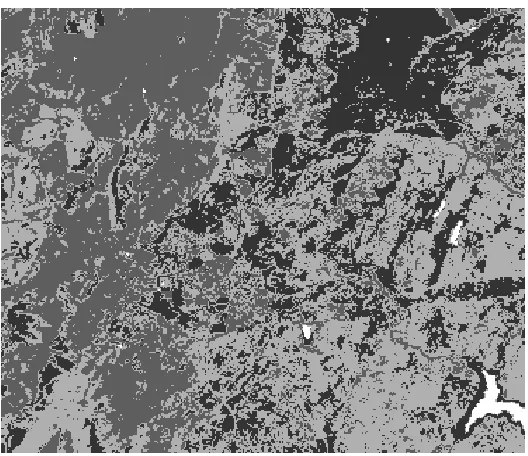
The latest GCS network trained with LEAE criterion has been labeled using the vegetation, water, and soil indexes previously exposed. There is one cluster of neurons that identifies water, one for vegetation, three for soil, and finally the single cluster that contains neurons that identify the two types of covers (vegetation and soil) has been labeled as mixed. Using this network, the original image has been processed and each pixel has been labeled using the method previously described. Fig. 12 shows this image displayed in four colors that identify the water, soil, vegetation and mixed covers.
Fig. 12. Water, vegetation and build-up indexes applied to the original image. Light gray color is associated to vegetation, white to water, dark gray to mixed, and black to soil covers.
4. Conclusions
two-dimensional output layer of the network makes it possible to visualize the relationships between the input patterns, and various grayscale graphics can be generated providing relevant information about the knowledge inherent to the multidimensional input space.
The proposed methodology applied to remote sensing data obtains a simplified model of an input space consisting of a high volume of pixels. This simplified model remains the most important information about the different land cover categories that can be identified in the image under study. The ability to generate various topographic maps from a GCS network trained with a remotely detected image is a powerful tool in the field of remote sensing and can be used in functions as common as the analysis of land cover, pixel classification or exploration of existing correlations between spectra bands.
This paper has proposed a new original topographic map, the combined component plane, which has proved that can be exploited to analyze the possible arithmetic combinations of spectral bands that can discriminate a specific land cover on a multispectral image, with a specific content and features, such as the spectral and spatial resolution, the land cover types or the weather conditions when the image was captured.
While the spectral indexes studied in the image used in the experiments are the classic for vegetation, water and soil covers, the proposed tool has demonstrated the ability to design new spectral indexes and validate its discrimination capacity for different types of land cover categories and sensors with other features.
References
Ceccato P, Gobron N, Flasse S, Pinty B, Tarantola S (2002). Designing a spectral index to estimate vegetation water content from remote sensing data: Part 1. Theoretical approach,
Remote Sensing Environment, 82, 188–197.
Chuvieco E, Cocero D, Riaño D, Martin P, Martínez-Vega J, de la Riva J, Pérez F (2004). Combining NDVI and surface temperature for the estimation of live fuel moisture content in forest fire danger rating, Remote Sensing of Environment, 92, 322–331.
Delgado S, Gonzalo C, Martínez E, Arquero A (2004). Improvement of Self-Organizing Maps with Growing Capability for Goodness Evaluation of Multispectral Training Patterns, Geoscience and Remote Sensing Symposium, IEEE International (IGARSS’04), Anchorage, Alaska, USA.
Delgado S, Gonzalo C, Martínez E, Arquero A (2007). Visualizing High-Dimensional Input Data with Growing Self-Organizing Maps, Lecture Notes in Computer Science, 4507, 580-587.
Fritzke B (1994). Growing cell structures – a self-organizing network for unsupervised and supervised learning, Neural Networks, 7 (1), 1441-1460.
He C, Xie D (2008). Improving the normalized difference build-up index to map urban build-up areas by using a semiautomatic segmentation approach. Geoscience and Remote Sensing Symposium, IEEE International (IGARSS’08), Boston, Massachusetts, USA.
Huete A R (1988). A soil-adjusted vegetation index (SAVI), Remote Sensing Environment, 25, 295-309.
Hui F, Xu B, Huang H, Yu Q, Gong P (2008). Modelling spatial-temporal change of Poyang Lake using multitemporal Landsat imagery, International Journal of Remote Sensing, 29 (20), 5767-5784.
Jackson T J, Chen D, Cosh M, Li F, Anderson M, Walthall C, Doriaswamy P, Hunt E R (2004). Vegetation water content mapping using Landsat data derived normalized difference water index (NDWI) for corn and soybeans, Remote Sensing Environment, 92, 475-482.
McFeeters S K (1996). The use of the normalized difference water index (NDWI) in the delineation of open water features. International Journal of Remote Sensing,17, 1425-1432. Pinty B, Verstraete M (1992). GEMI A nonlinear index to monitor global vegetation from
satellites, Vegetation, 101, 15-20.
Rouse Jr J W, Haas R H, Schell J A, Deering D W (1973). Monitoring vegetation systems in the Great Plains with ERTS, Third Earth Resources Technology Satellite-1 Symposium (Eds. S. C. Freden, E. P. Mercanti, & M. Becker), I, 309–317.
Tucker C J (1979). Red and photographic infrared linear combinations for monitoring vegetation, Remote Sensing of Environment, 8, 127–150.
Verstraete M. Pinty B (1996). Designing optimal spectral indexes for remote sensing applications, IEEE transactions on Geosciences and Remote Sensing, 34 (5), 1254-1265. Zha Y, Gao J, Ni S (2003). Use of normalized difference built-up index in automatically