A Valuation Method for Credit Default Swaps Using an Extended Version of the Merton Model

(1)

A Valuation Method for Credit

Default Swaps Using an Extended

Version of the Merton Model

Master’s Thesis in Financial Economics

Author:

Eilif Drageseth

Academic Supervisor:

Cristina Danciulescu

Norwegian University of Science and Technology Department of Economics

(2)

Abstract

This thesis proposes a credit risk model for credit default swap (CDS) valuation. The standard Merton (1974) model is extended to implement a stationary leverage ratio, a stochastic asset drift rate, and a stochastic, mean reverting volatility rate. The CDS valuation is performed by applying the discounted cash flow method to the credit risk model. The model is investigated in Matlab, using Monte Carlo simulations to analyze the sensitivity of the modeled CDS term structures to changes in the value of the input parameters. The results show that the proposed model generates higher CDS spreads than the standard Merton model.

Preface

This thesis is the completion of my two-year MsC. program in Financial Economics at the Department of Economics, NTNU. The writing of the thesis has been an informative process, and has provided several academic challenges. The work has provided me with a valuable experience which I will benefit from in the future.

I would like to thank my thesis supervisor Cristina Danciulescu for great academic sup-port, and for always taking the time to answer my questions and aid me in the work with this thesis. I would also like to acknowledge Hanne Sofie Otterlei for proof reading and linguistic input.

(3)

1 Introduction

A CDS contract is a credit derivative that pays off if there is a default on the underlying bond. For lenders, it basically functions as an insurance policy against default. The owner of the CDS contract will have to pay an insurance premium to the issuer of the CDS contract, who is normally referred to as the writer of the contract. If a default occurs, the CDS writer is obligated to buy the defaulted bond from his CDS counterpart for the bond’s face value. The size of the premium will of course depend on the probability of default for the underlying bond, but also on other factors, such as the expected value of the underlying bond following a default.

The market for Credit Default Swaps (hereafter shortened to CDS) is relatively new, having been introduced in the early 1990’s (McDonald, 2006). Since then it has increased

rapidly in size, most notably during the last decade. According to Hull (2012), the

market for credit derivatives increased from a total notional principal of approximately $800 billion in 2000 to an impressive $32 trillion in 2009. The CDS contracts are the most actively traded of the credit derivatives, accounting for as much as 45% of the market in 2004 (Zhu, 2006). This market increase is accompanied by a growing field of research on the subject, but there are still questions to be answered.

One of the reasons why the CDS contracts have become so popular is because of their ability to act as an insurance against default for bond owners. If an investor has a long bond position, a perfect hedge would be to buy a CDS contract with the same bond as the underlying security. He will then pay a premium to the CDS writer, but he will in turn receive the face value of the bond in case of default. Seeing as you do not need to own the underlying bond in order to buy a CDS contract, the CDS can also be used for speculative purposes. There is evidence that the notional principal of CDS contracts can exceed the total amount of debt issued by the bond issuer, usually titled the reference entity (Hull, 2012). As an example, when Lehman Brothers defaulted in 2008 there was a total worth of $400 billion of CDS contracts in circulation with Lehman Brothers as the reference entity. The total debt outstanding was only $155 billion. This indicates that speculative usage of CDS contracts occur on a relatively large scale. The CDS can in a way function as a substitute for a short position in the underlying bond. This creates extended investment options to investors since short selling of corporate bonds is not always possible.

To value a CDS contract, a valuation model is needed. The probability of default for the reference entity is an important factor in determining the fair CDS premium. One way of finding these probabilities is to use a model for valuing corporate bonds. In 1974 Robert C.

(6)

Merton published an influential paper on the pricing of corporate bonds (Merton, 1974). He uses the famous Black & Scholes (1973) model to price corporate debt. Merton’s paper presents one of the earliest of the so-called structural models for pricing defaultable bonds. An advantage of these models is that they are based on sound financial theory. The results also largely give intuitive interpretations. They are, however, dependent on a series of assumptions, some of which are more realistic than others. Another class of models that have been popular in more recent years is the reduced form, or hazard rate models, such as Duffie & Singleton (1999). These models utilize default probabilities or hazard rates to induce the bond price. Default in the reduced form models is effectively treated as a pure jump process. The hazard rate models implement complex structures to explain patterns observed in empirical data. They do not necessarily have a sound theoretical base in the background, and this complicates the interpretation of the model. The reduced form models often outperform structural models for shorter time spans, but the structural models have an advantage as the time span is increased.

The CDS market is today considered a better indicator of creditworthiness than the bond market (Zhu, 2006). As Zhu (2006) shows, the CDS market appears to be leading the bond market following new information. Discrepancies between the bond and the CDS market are also quite persistent in his data, where only about 10% of such discrepancies were removed on average during one business day. This is interesting because, from a theoretical view, such discrepancies should not occur. Furthermore, the findings of Yu (2005) suggest that there might be profitable arbitrage trading strategies from exploiting imbalances between predicted and observed spreads in the CDS market when using a structural model. In an efficient market such arbitrage strategies should not exist. This implies that the market for CDS contracts might be inefficient. The CDS market is thus an ideal subject for further studies.

This thesis proposes a method for CDS valuation based on the Merton (1974) model, albeit with three important extensions. The classic Merton model assumes that no new debt is issued during the lifetime of the bond in question. This is not consistent with the real world behavior of firms. Collin-Dufresne & Goldstein (2001) propose implementing a time-varying stationary leverage ratio in a structural model to work around this problem. The Merton model also assumes a constant volatility and drift rate for the assets of the firm. Again, this is not very consistent with the real world. Constant volatility rates are very rare, and a number of different approaches to model time-varying volatility have been proposed. This thesis implements a stochastic mean reverting volatility rate in the form of a Cox-Ingersoll-Ross process. This is a common way of modeling time-varying volatility, and is used in influential papers such as Heston (1993). The drift rate of the assets of the firm can be interpreted as the growth rate of the firm. The growth rate is usually

(7)

not immune to macroeconomic shocks or other influential events. Additionally, expected growth can be declining or increasing over time. The model is therefore extended to account for a stochastic drift rate process. By making some of the underlying assumptions more realistic, the new model will hopefully give more accurate predictions.

The thesis is divided into six chapters. Chapter 2 introduces some important results that are needed to develop the valuation model. Chapter 3 derives the standard Merton (1974) model and defines the CDS contract. It also presents a way of valuing the CDS contracts, building on the work by Hull & White (2000). Chapter 4 then moves on to implement the new extensions in the model. The thesis uses a Monte Carlo simulation process to obtain simulated results for CDS term structures. The way this is done and the calibration of the model is explained in chapter 5. Chapter 5 also contains the results from the Monte Carlo analysis. A conclusion of the work is provided in chapter 6.

(8)

(9)

2 Important Concepts and Definitions

2.1 The Concept of Brownian Motion, Log-Normality and Itô’s

Lemma

This section builds in part on a textbook by Hull (2012). Some of the underlying concepts of the Merton (1974) model need to be understood before introducing the model. First of all, it is assumed that the assets of the firm follow a stochastic process known as the Markov process. The Markov process is a continuous time process where only the current value of the variable influences its future value. All historic values are irrelevant, so the future value is not dependent on the path of the process. For stock prices, the Markov process is consistent with the weak form of market efficiency: all information from past prices are accounted for in the current price. Several studies have found the weak form of market efficiency to hold in stock markets (Bodie, Kane & Marcus, 2009).

The next underlying concept that needs to be explained is the Wiener process. The Wiener process is a special case of the Markov process where the process is changing by an average of zero per unit of time, with a variance of one. This means that the value in the next period is the current value plus a random generated number from a standard normal distribution. The Wiener process is also often referred to as a standard Brownian

motion. The change in a random variable (z), ∆z, for a small time period, ∆t, is then

given by:

∆z=√∆t, (2.1)

where is a random number drawn from a standard normal distribution.

The mean change per unit of time in a stochastic process is called the drift rate of the process. In the same manner, the variance per time unit is called the variance rate. A

generalized Wiener process for a random variable, x, will be:

dx=adt+bdz, (2.2)

where a and b are constants representing the drift rate and the variance rate of the

process, respectively. If ais positive, the process will generally be trending upward, while a negative drift rate will produce a process trending downwards. The mean of the process is a∆t, while its standard deviation is b√∆t. Applied to a stock price, S, with a drift rate, µ, and a variance rate of σ2_{, the process can be stated as:}

(10)

Equation (2.3) is called a standard geometric Brownian motion. In the model proposed in this thesis (see chapter (4)), the drift and variance rate is allowed to change over time.

If the drift and variance also depended on the underlying variable, x, the process would

be given as:

dx=a(x, t)dt+b(x, t)dz (2.4)

Equation (2.4) is known as an Itô process.

To solve the Black & Scholes (1973) equation (see chapter 3), the application of Itô’s lemma is needed. IfGis a differentiable function ofx, the change inG,∆G, resulting from

a change in x,∆xcan be found by using a Taylor series expansion of the approximation:

∆G= dG

dx∆x (2.5)

Assuming that the third and higher order approximations are close to zero, the change in a function G(x, t)can be expressed as:

∆G= ∂G ∂x∆x+ ∂G ∂t∆t+ 1 2 ∂2_G ∂x2∆x 2 ₊ ∂2G ∂x∂t∆x∆t+ 1 2 ∂2_t ∂t2∆t 2 _(2.6)

When the time steps, ∆t are sufficiently small, the term ∆t2 _{will be approximately equal}

to zero. The cross product ∆x∆t is also assumed approximately equal to zero. Using

equation (2.4), the term ∆x2 _{is given by:}

∆x=a(x, t)x∆t+b(x, t)x√∆t (2.7)

∆x2 =b2x∆t (2.8)

This result arises from the assumptions that ∆t2 ≈ 0 and ∼ N(0,1), where N(0,1) is

the standard normal distribution with a mean equal to 0 and a variance of 1. Because

E[] = 0, the following is obtained: V ar() = E[2_]₋₍_E_[_])2

= E[2_{] = 1}_{. Rewriting}

equation (2.6) when the limits of ∆x and ∆t approach zero, leads to equation (2.9):

dG= ∂G ∂xdx+ ∂G ∂tdt+ 1 2 ∂2G ∂x2b 2_xdt _(2.9) dG= ∂G ∂x(axdt+bxdz) + ∂G ∂t dt+ 1 2 ∂2_G ∂x2b 2 xdt (2.10) dG= ∂G ∂xax+ ∂G ∂t + 1 2 ∂2_G ∂x2b 2_x dt+∂G ∂xbxdz (2.11)

G is a process that is affected by the same source of uncertainty asx, namely the Wiener

process dz. The result in equation (2.11) is known as Itô’s lemma.

(11)

(2.3), applying Itô’s lemma to the function G = lnS gives the following process for the change in G:

dG= (µ−0.5σ2)dt+σdz (2.12)

Given that both µ and σ are considered constant here, the change in lnS between time

0 and T is normally distributed. When this is the case, the stock price is said to be

lognormally distributed. An expression for the expected future value of the stock price can then be derived from equation (2.12):

lnST −lnS0 ∼ N [µ−0.5σ2]T, σ2T (2.13) lnST ∼ N lnS0+ [µ−0.5σ2]T, σ2T (2.14) ST =S0expN [µ−0.5σ2]T, σ2T (2.15) E[ST] =S0e(µ−0.5σ 2₎_T (2.16)

The last concept to be introduced before turning to the valuation model is the concept

of risk-neutral valuation. This is an easy way of calculating probabilities and prices

independent of differing risk premiums. It basically assumes that all investors are risk neutral, meaning they do not demand a risk premium for risky investments. All securities thus have a payoff that is normalized to the risk free rate. When the payoff is the risk free rate, the discounting can also be done at the risk free rate. The reason why this is possible is that when using real expected risk adjusted returns, the discounting also needs to be done at the proper risk adjusted rate. It so happens that discounting at the risk adjusted rate exactly offsets the risk adjusted expected return, giving the same results as the risk neutral calculation. The risk neutral probability of default will generally not be equal to the real world probability, but the calculated security values will be the same.

(12)

(13)

3 Credit Risk and Credit Default Swaps

To value CDS contracts the way this thesis suggests requires a model of credit spreads on bonds. The credit spread is the premium the borrower must pay to the lender to compensate for the default risk. This premium is defined as the excess return on the investment over a risk free alternative. The credit spread, s, can thus be expressed as:

s(t, T) = y(t, T)−r, (3.1)

where y is the yield on the bond in question and r is the return on a risk free bond. t is the time from which the contract is valued, while T is the maturity date. When borrowing money, a company that is considered likely to go bankrupt will naturally be required to pay a higher premium than more financially robust companies. The risks associated with lending money can be many. A lender will have to consider the macroeconomic risk of the sector in question, the risk of the company making bad decisions leading into financial distress, inflation risk, and more. Determining a fair premium is thus not always an easy task, and over the years there have been several alternative attempts to model credit spreads. The most famous approaches are perhaps the structural models such as Merton (1974), and the hazard rate (or reduced form) models such as Duffie & Singleton (1999). The structural approach explicitly models the firm value using option pricing theory. Hazard rate models on the other hand, models default as a random stopping time with stochastic arrival intensity. This thesis uses the framework of the Merton model as its base model.

3.1 The Merton Debt Pricing Model

The famous Black & Scholes (1973) option pricing model presented a new and more robust way of valuing options on common stocks. In their paper, they also discuss the possibility of using the same framework to value corporate bonds. If the bonds are pure discount bonds (no coupon payments), then “[i]n effect, the bond holders own the company’s assets, but they have given options to the stockholders to buy the assets back” (Black & Scholes, 1973, p. 649-650). It is also possible to adjust for coupon payments by considering valuation models for compounded options, but that is beyond the scope of this thesis. Robert C. Merton (1974) elaborates further on these ideas, adjusting the Black & Scholes model to price corporate bonds. Using the definitions in table 1, the payoff from owning equity is given as:

(14)

Table 1: Definitions

V0: Value of the company’s assets at time 0 D: Debt repayment due at time T

VT: Value of the company’s assets at time T σV: Volatility of the assets

E0: Value of the company’s equity at time 0 σE: Volatility of the equity

ET: Value of the company’s equity at time T T: Time of maturity

If the firm value is larger than the debt value at the time of maturity, the equity holders exercise the option to receive the remaining value after the debt is cashed out. If the firm value is less than, or equal to the debt value at the time of maturity, the equity holders choose not to exercise their call option. The shareholders will then receive zero money as all value is transferred to the debt holders. Consequently, the debt value can, in option pricing terms, be considered as the strike price of the call option. Using the same notation, the bond holders will receive min[VT, D]. If the firm value is larger than

the owed amount, the debt will be repaid. If the firm value is less then the owed amount, the lenders will sell the firm’s assets and receive the firm value. A few key assumptions are needed for this framework to be valid. Following the original paper of Merton (1974), these assumptions are:

• No transaction costs, taxes or indivisible assets exist.

• Every investor can buy or sell as much of an asset as he desires at the market price.

• Borrowing and lending can be done at the same rate of interest.

• Short-sales are allowed for all assets.

• Trading takes place in continuous time.

• The Modigliani-Miller theorem holds, meaning that the firm value is independent

of capital structure.

• There exists an investment opportunity with a constant risk free rate of return.

• The firm value process can be described as a geometric Brownian motion with drift:

dVt =µVtdt+σVtdz, (3.3)

whereV is the firm value,µis the drift rate of the firm’s assets andσis the volatility

rate of the assets. z is a standard Wiener process.

(15)

Assuming a security whose market value F can be stated as a function of the firm value

and time, F = f(V, t), and using Itô’s lemma from equation (2.11) with equation (3.3)

gives the following process for F:

dF = ∂F ∂V µV + ∂F ∂t + 1 2 ∂2_F ∂V2σ 2_V2 dt+ ∂F ∂V σV dz (3.4)

Note that both (3.3) and (3.4) are exposed to the same risky component,dz. This property

makes it possible to form a risk free portfolioΠ, with the portfolio weightsaandb. ais the share of the underlying asset in the portfolio, while b is the share of the new security, F.

As usual, the portfolio weights must add up to one,a+b= 1. Solving this problem yields

a = ∂F_∂V and b = −1. Due to the riskless nature of this portfolio, it must have a return

equal to the risk free rate (in the absence of arbitrage). This means that dΠ = rΠdt.

Combining these results give the ‘Black-Scholes-Merton differential equation’:

∂F ∂t +rV ∂F ∂V + 1 2σ 2_V2∂2F ∂V2 =rF (3.5)

As Merton (1974) states, this equation is:

[...] a parabolic partial differential equation for F, which must be satisfied by

any security whose value can be written as a function of the value of the firm

and time. Of course, a complete description of the partial differential equa-tion requires in addiequa-tion to [equaequa-tion (3.5)], a specificaequa-tion of two boundary conditions and an initial condition. It is precisely these boundary condition specifications which distinguish one security from another (e.g., the debt of a firm from its equity). (p. 452)

Solving the equation for a European call option gives the standard Black-Scholes-Merton model: E0 =V0N(d1)−De(−rT)N(d2) (3.6) d1 = ln(V0/D) + (r+σ2V/2)T σV √ T (3.7) d2 =d1−σV √ T (3.8)

Here, N(·) is the standard normal cumulative distribution function. The model uses risk

neutral probabilities, something which is handy when valuing CDS contracts. For an intuitive interpretation, equation (3.6) can be rewritten as:

E0 =e−rT V0N(d1)erT −DN(d2)

(16)

The first part within the paranthesis of equation (3.9) can be interpreted as the expected cash inflow from owning the option. In other words, it is the expected value of a variable

that pays VT|VT > D and 0|VT ≤ D. The second part of the paranthesis in equation

(3.9) is the strike price times N(d2). This is the expected value of the payment that is

due if the option is exercised. N(d2) can accordingly be interpreted as the risk neutral

probability that the option will be exercised, triggering the payment of the strike price. Since there are only two outcomes, exercise or no exercise, the probability of default (no exercise) can be found as 1−N(d2) =N(−d2).

The probability of default is decisive in determining the size of the bond’s risk premium. The price of a bond today should be equal to the face value of the bond discounted at the proper risk adjusted rate, also known as the yield to maturity (still assuming no coupons). Usually, the yield is determined from the observed market data by finding the yield that solves the following equation:

B(t, T) = De−y(t,T)(T−t), (3.10)

whereB is today’s bond price. The credit spread of the bond can be found by rearranging

the above equation and using the definition of the credit spread from equation (3.1):

s(t, T) = 1 T −tlog D B(t, T) −r (3.11)

From this equation one can find the direction of change in credit spreads from changes in the other variables. The ceteris paribus effects are:

• ∂s

∂T−t S 0: Increasing the time to maturity would appear to lower the spread

ac-cording to equation (3.11). Because B is a function of the time to maturity, this is, however, not the final answer. From equation (3.10), it is obvious that increasing the time to maturity lowers the current bond value. There are thus two forces in action at the same time, pulling the spread in different directions. Whichever is the strongest of the two, will depend on the other elements in equations (3.10) and (3.11). It would, however, generally make sense to assume that a longer maturity should increase the bond spread, being that it is harder to make predictions as the time horizon is expanded. This uncertainty will increase the risk, and hence the risk premium known as the spread.

• ∂s

∂D > 0: A higher face value of debt increases the chances that the company will

not be able to pay their debt. For this reason, the spread increases with the face value.

(17)

• ∂s

∂B < 0: A low bond value today is consistent with a high credit spread. The

bond value today and the credit spread are closely linked, and this should be as anticipated.

• ∂s

∂r < 0: A lower risk free interest rate will, of course, increase the credit spread

given that the yield is unchanged. However, if the risk free rate is lowered and the riskiness of the bond is unchanged, the yield is also likely to decrease. The bond value should then increase, leaving the credit spread unchanged.

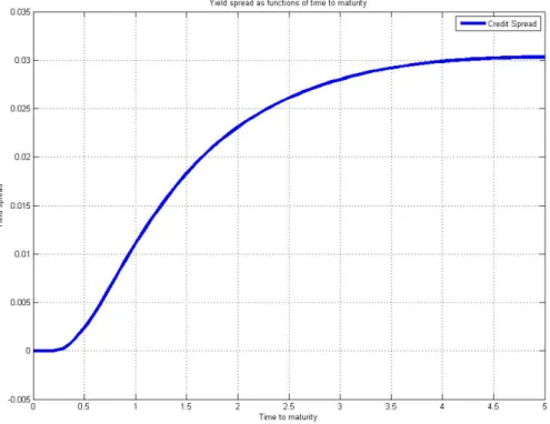
Figure 1 plots a simulated credit spread against the time to maturity using the Merton model. The model typically predicts an upward sloping credit spread with diminishing growth.

Figure 1: Simulated Credit Spread From The Merton Model. The parameter values used in the simulation are: T = 5, V = 100, D = 40, r= 0.05, σ= 0.35

3.2 The Credit Default Swap: Definition and Contractual Terms

A CDS is a credit derivative contract that has a payoff contingent on default or no-default on a pre-specified bond, issued by a company referred to as the reference entity. The writer/seller of the CDS receives a premium on specified dates (typically each quarter), and must in return buy the the underlying bond for its face value in the case of default.

(18)

If there is no default by the reference entity before the maturity date of the CDS, the payoff to the CDS seller is the accrued premium payments from the writing date to the maturity date. If the reference entity does default before maturity, the seller receives the premium payments up to default, but must pay the buyer the difference between the bond’s market value and its face value at the time of default. The CDS can be settled either physically, by the delivery of the bond, or by cash settlement. These two forms of settlement will generally not affect the payoffs from the CDS. Cash settlement is often necessary, however, due to the fact that the total CDS notional amount in the market sometimes exceeds the total outstanding debt issued by the reference entity.

The buyer (writer) of a CDS will lose (earn) money if the reference entity does not default, and will gain (lose) if a default occurs. For a reference entity that is not likely to default, the CDS seller will demand only a relatively small premium. For companies that are considered likely to find themselves in financial distress, the demanded premium will be relatively high to reflect the probability that the default payment will be triggered. If the CDS buyer is long in the underlying bond, the CDS can be viewed as an insurance policy against loss on the bond position. Because there is no need for a CDS buyer to hold a long position in the underlying bond, the CDS contract can be used for speculative purposes and functions as a bet on the default probability of the reference entity.

A long CDS position can also be synthetically replicated by entering in a long position in a par risk free bond (i.e. T-bills or similar) with the same maturity as the underlying, together with a short position in the underlying risky par bond. This will give a negative payoff equal to the credit spread of the defaultable bond up until maturity. At maturity the face value is received on the risk free bond, and passed on to the buyer of the defaultable bond. If a default occurs on the risky bond before the maturity date, the risk free bond can be sold, and the risky bond bought back. This renders a payoff equal to the face value discounted with the risk free rate, minus the market value of the risky bond. Such a synthetic replication gives rise to an arbitrage pricing model for the CDS premium. If the payoff from a CDS and this synthetic CDS position is equal, then standard financial theory suggests that they should also be priced equal after considering any transaction costs. Short selling of bonds can, however, be difficult to achieve, and this parity condition does not necessarily hold (Hull, Predescu & White, 2004).

To enter in a CDS contract usually requires no initial payment. The premium is set so that the expected payoff at the initiation day is equal to zero. In the second hand market the value of the CDS will generally be non-zero due to changing market conditions and expectations. Because of difficulties involved in the short selling of bonds, the CDS is an attractive asset class for investors who want to make a bet on the debt of a company. As

(19)

a result, the CDS market is often more liquid than the bond market itself. Studies have shown that the CDS market captures new information as much as two to three weeks faster than the bond market (Zhu, 2006), underlining this difference in liquidity.

Most CDS contracts are standardized by the International Swaps and Derivatives Asso-ciation (ISDA). One of the most important aspects of these contracts is the definition of a credit event. Under the original ISDA agreement from 1999 there were six different actions that qualified as credit events (Packer & Zhu, 2005; Tolk, 2001):

1. Bankruptcy 2. Failure to pay 3. Restructuring 4. Repudiation/moratorium 5. Obligation default 6. Obligation acceleration

Moody’s argue that some of these actions appear to have unwanted consequences (Tolk, 2001). The CDS buyers will be driven by moral hazard, and it can be difficult to keep them from calculating losses and defining credit events in a favourable way. An example is the inclusion of restructuring as a credit event, which Packer & Zhu (2005) claim is the most challenging of the credit events to contract for within CDS contracts. This is due to the fact that restructuring often constitutes a ‘soft’ credit event, meaning that the loss to the obligation owner is not obvious. Another point is that restructuring can retain a complex maturity structure for the still outstanding obligations of the reference entity. This may cause debt issues of different maturities to remain outstanding with different values. As an example of these unwanted properties Packer & Zhu (2005) uses the restructuring event of Conseco Finance in 2000:

[...] the bank debt of Conseco Finance, restructured to include increased

coupons and new guarantees, and thus not disadvantageous to holders of the previous debt, still constituted a credit event and triggered payments under the ISDA guidelines. (page 91)

Because of this flaw in the standardized contract, new versions were developed. The original standard is now referred to as “Full Restructuring”, or simply FR. In 2001 the so-called “Modified Restructuring” (MR) standard was introduced. These contracts closed

(20)

the gaps in the original contract by limiting the deliverable obligations to those that have a maturity of 30 months or less after the restructuring event. Any restructuring is still considered a credit event, but due to the limitations on which bonds are deliverable it is no longer as easy to exploit the contract.

Several investors, particularly in Europe, argued that the restrictions imposed by the MR contracts were too harsh. ISDA consequently published a new standard contract in 2003 called “Modified Modified Restructuring” (MM). In this clause the restrictions from the MR contracts are given some relaxation. The restructured obligations can have a maturity of up to 60 months after the restructuring, while the 30 month rule still applies for all other obligations. The last standard is the contract with no restructuring (NR). This clause does not consider restructuring as a credit event at all. As Packer & Zhu (2005) show, the premium on an NR contract will be lower than any of the other contracts. The broader the definition of default, the higher the risk that the bond will be defaulted, and hence the higher premium is demanded by the CDS writer. The most expensive contract is therefore the FR, followed by the MM contract, the MR contract and, finally, the cheapest NR standard. The different contractual types are very important when pricing a CDS. This thesis will however assume that all contracts are of the same type, and so sidesteps this issue. A default is here defined as in the Merton (1974) model: the reference entity defaults if the total amount of debt outstanding at maturity is higher than the value of the firm’s assets. There is thus no room for so-called ‘soft’ credit events in this framework.

3.3 CDS Valuation

The fact that a CDS contract can be replicated synthetically using par discount bonds, gives rise to a parity relationship between bond and CDS spreads (Duffie & Singleton, 1999; Hull et al., 2004; Zhu, 2006). The CDS is replicated by entering a short position in the underlying risky bond and a long position in a risk free bond with the same maturity and face value. As a result, the investor will receive the risk free interest rate, but must pay the yield on the risky bond. The investor is left with a negative cash flow equal to the credit spread on the risky bond. If, at maturity, there is a default on the risky bond, the investor will have to repay only the recovery value of the risky bond. He will receive the face value from the risk free bond, and is left with the difference between the two. This is exactly the same payoff structure as that from a CDS contract. In the absence of arbitrage, the CDS spread should thus be equal to the bond spread.

Entering in such a synthetic CDS contract is, however, rarely possible. As Zhu (2006) points out, short sales of corporate bonds are practically forbidden. In addition, time

(21)

varying interest rates complicate matters, while suitable par discount bonds are not always available. In addition, the CDS market appears to be more liquid than the bond market, giving rise to a possible difference in liquidity premium. A better valuation method for CDS contracts is therefore required.

Hull & White (2000) suggest a valuation method based on the risk neutral probability

of default. They suggest finding the risk neutral probability, p, from observable data by

solving the following equation:

D(1−R)pe−rt =s, (3.12)

where, as before,D is the face value of the bond,Ris the recovery rate in case of default,

r is the risk free rate ands is the excess return over the risk free rate on the risky bond. Here it is assumed that the difference between the value of a risk free bond and a risky corporate bond equals the present value of the costs of default. The probability of default can also be retrieved from the Merton (1974) model of credit spreads, and that is the approach used in this thesis. The CDS valuation model thus builds on a combination of the Merton model and Hull and White’s methods.

The premium payments on the CDS can in principle be divided into two parts: the payment when no default has occurred, and the accrual premium payment in the case of default. At default, the CDS contract is settled, and the owner is thus not obliged to pay any residual premiums. The two parts can be stated as:

Dc0,T∆ti1{τ >ti} Dc0,T(τ−ti−1)

τ is defined as the time of default, while c0,T is the CDS spread of a contract at time 0

with maturityT. The indicator function 1{τ >ti} is equal to 1 given that no default occurs

before time ti, and zero otherwise. The former of the two expressions is the premium

payment when there is no default, while the latter expression is the accrual payment following a default. Combining the two expressions, the expected present value of cash outflows for the CDS owner can be written as

EQ " _z X i=1 Dc0,t∆tie−rti1{τ >ti}+Dc0,t(τ −ti−1)e −rτ 1{ti−1<τ <ti} # (3.13)

Here, EQ _{is the martingale measure, or the risk neutral expectation operator. The CDS}

(22)

default has occured:

EQD(1−R)e−rτ1{τ≤T}

(3.14) The fair spread can then be found by finding the premium payment that equates the expected in and outflow of cash:

EQ " _z X i=1 Dc0,T∆tie−rti1{τ >ti}+Dc0,T(τ−ti−1)e −rτ 1{ti−1<τ <ti} # (3.15) =EQ D(1−R)e−rτ1{τ≤T} c0,T = EQD(1−R)e−rτ1{τ≤T} EQ _z P i=1 D∆tie−rti1{τ >ti}+D(τ −ti−1)e −rτ₁ {ti−1<τ <ti} (3.16) c0,T = EQ (1−R)e−rτ1{τ≤T} EQ _z P i=1 ∆tie−rti1{τ >ti}+ (τ −ti−1)e −rτ₁ {ti−1<τ <ti} (3.17)

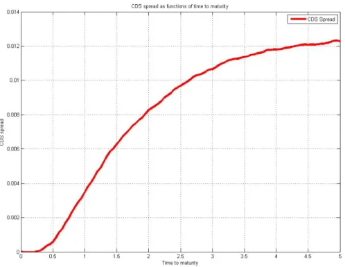
The expectation operator indicates that the CDS spread is affected by the default prob-ability. The CDS spread is thus increased when the debt level is increased or the firm value decreases. The expected recovery value will of course also have an effect. If the expected recovery value is high, the spread will be fairly small. As the time to maturity increases, it is more difficult to make predictions, resulting in increased uncertainty. The CDS spread therefore usually inhibits the same diminishing growth property as the bond spread. Using the simulated risk neutral probability of default from the Merton model, a simulated CDS spread is plotted in figure 2.

(23)

Figure 2: Simulated CDS Spread. Parameter values are: T = 5, V = 100, D = 40, r = 0.05, σ= 0.35, R= 0.5

(24)

(25)

4 An Extended Credit Risk Model for CDS Valuation

As discussed in chapter 3.3, the parity condition between bond spreads and CDS spreads is generally not expected to hold. Many market participants use models such as the one presented in chapter 3 to estimate the correct CDS spread. In a well functioning capital market there should be no arbitrage opportunities. Yet Yu (2005) finds several seemingly profitable arbitrage trading strategies exploiting mispricing in the CDS market. His findings suggest that the strategies are profitable also after considering transaction costs. It seems then, that current valuation techniques are dissatisfactory, and that a better way of valuing the CDS contracts are desirable.

There has been an ongoing debate in financial scientific journals regarding the accu-racy of structural approaches building on the Merton (1974) model (see, among others, Sobehart & Keenan, 2002, for a discussion). Different researchers have approached the subject in different ways, but the general conclusion seems to be that the original model can be improved by making some extension to the framework (see for instance Du & Suo, 2003; Falkenstein & Boral, 2001; Hull, Nelken & White, 2004). Quite a few such exten-sions have been proposed. This thesis builds on the seemingly successful extension made by Collin-Dufresne & Goldstein (2001), implementing a mean reverting process for the debt value. Furthermore, the volatility rate of the firm’s assets is also modeled as mean reverting. Finally, the extended model in this thesis incorporates an uncertain drift rate for the assets of the firm. This should, in theory, give more realistic results than the standard model described in chapter 3.

4.1 A Mean Reverting Debt Level

The implementation of a mean reverting debt level in the Merton (1974) framework follows the work of Collin-Dufresne & Goldstein (2001). The standard Merton model assumes that the debt level of the company is kept constant in absolute terms until the debt is repaid. This simplification is not very realistic. It is beneficiary for most firms to issue some debt, due to the so-called tax shield effect (Berk & DeMarzo, 2011). The tax shield occurs because companies pay tax on their income after interest payments have been deducted. This way, the total value available to the owners of the company (both debt and equity) is larger than it would have been with equity, only. At the same time, issuing debt increases the risk of bankruptcy. In a perfect, frictionless market, bankruptcy would simply be a transfer of assets from the equity holders to the debt holders. In the real world, however, bankruptcy can be a long and complicated process. A fee has to be paid

(26)

to the lawyers who manage the bankrupt’s estate, the assets might not be sellable without incurring transaction costs, and some assets such as human capital and customer relations might disappear altogether. Because of these direct and indirect costs of bankruptcy, most companies try to avoid financial distress by limiting their liabilities. The costs and gains of issuing debt leads to an optimal capital structure, and it is therefore common for companies to have a target level for the debt to value ratio (Berk & DeMarzo, 2011; Collin-Dufresne & Goldstein, 2001). If the firm value rises, it would make sense to issue more debt to keep the debt ratio at optimum. Equivalently, if the firm value decreases, the company would want to refrain themselves from issuing new debt so that they will reach their target level again in the near future.

In addition to the mean reverting nature of the debt process, the company might also come across a situation where they urgently need liquidity. In such a scenario the company might be forced to issue new debt even though they are above their target level. In the same manner, they may find themselves in a situation where there are no profitable investment options. If they cannot invest their existing cash reserves efficiently, it makes no sense to borrow more. Because of this uncertainty, the debt level should not just be mean reverting, it should also be volatile.

In the extended model, the debt process is given as:

dDt=kD(Dtarget−Dt)dt+σDdztD (4.1)

Here, kD is the mean reversion coefficient, Dtarget is the debt target level, D is the debt

value, σD is the volatility of the debt process and zD is a standard Wiener process. As

long as 0 < kD < 1 this process will be stationary, meaning that the debt will always

revert towards its long term value following a deviation. The volatility is assumed strictly

positive, meaning that the debt process is uncertain. The size of the volatility rate

determines how much the debt level is affected by shocks from the Wiener process, zD_.

When a shock pushes the debt level away from the target level, the mean reversion part comes into effect and pushes the debt level back to its target.

4.2 A Mean Reverting Volatility Rate

One of the less likely underlying assumptions of the Black & Scholes (1973) framework, is the constant volatility rate. Fisher Black himself noted this early on, stating that “Suppose we use the standard deviation of possible future returns on a stock as a measure of its volatility. Is it reasonable to take that volatility as constant over time? I think not”

(27)

(1976). The volatility is changing with both firm specific and macroeconomic conditions. Volatility clustering, the tendency for volatility to be high (or low) in concentrated periods, is also a well documented phenomenon in financial markets (Brooks, 2008; Hull, 2012). This suggests that the volatility should be modeled as a time-varying process.

Hull (2012) suggests the following process to describe the volatility rate of an asset:

dV =a(VL−V)dt+ξVαdz, (4.2)

whereV is the variance rate,VLis the long term variance rate andais the mean reversion

coefficient. ξ is the volatility rate of the process, and z is a standard Wiener process.

Equation (4.2) models the variance as mean reverting to a level VL at a speed of a per

period following shocks from the Wiener process. The size of the shocks are determined

by the volatility rate, ξ, and the parameter α. According to Hull (2012), the pricing of

instruments with less than one year to maturity is not significantly affected by introducing a stochastic volatility process. The effect is growing with the time to maturity, however, and the typical CDS contract has a contract length of five years. Accordingly, a non-constant volatility rate could have a significant impact on the CDS valuation.

Setting α = 0.5 in equation (4.2) leads to a standard Cox-Ingersoll-Ross (CIR) process.

Using the notation from previous chapters, the volatility process will look like this:

dσt= (α−kσσt)dt+η √

σtdztσ (4.3)

αin equation (4.3) is the adjusted long run mean of the volatility,kσ is the mean reversion

speed of the process, whileη is the volatility rate of the volatility process. zσ _{is as usual a}

standard Wiener process. The CIR process can never become negative and is well suited for modeling volatility rates. It is also often used for this purpose (see, among others, Heston, 1993).

4.3 A Stochastic Drift Rate

The drift rate of the firm value is also assumed constant in the original Merton (1974) model. In the real world, however, firms generally do not have constant growth prospects. The growth rate is usually time-varying, and it would make sense to model it as a stochas-tic process (Gao & Chen, nd). The extension models the drift rate as a standard geometric Brownian motion (GBM):

(28)

Here, aandbare the drift rate and volatility rate of the drift rate process, respectively. zµ

is a standard Wiener process. By modeling the drift rate process as a geometric Brownian motion, the growth rate of the firm is uncertain. How much it changes over time is in part controlled by the parameter values. If the company is expected to increase their

growth rate over time, a value of a between zero and one would make sense. This could

be a probable scenario for a new company with strong growth prospects. The drift rate could also be expected to decline over the forecast period. A former growth prospect that are establishing itself as a stable major corporation might be expected to have declining

growth for a certain period of time. If so, the parameter a should be somewhere between

zero and minus one. For many companies the drift rate is expected to be relatively stable.

For such companies, the drift parameter ain the drift rate process should be set equal to

zero. This would make the drift rate process non-trending, but it will be stochastic due to the uncertainty in the latter part of equation (4.4).

For most established companies the volatility rate of the drift process will be a more interesting parameter than the trend of the process. For these companies, a trending drift rate is non-probable. An uncertain drift rate, on the other hand, is rather likely. It is generally assumed that the volatility rate is non-negative. If it is positive, the drift rate is allowed to be influenced by random shocks from the Wiener process. These shocks can represent different firm specific, sector specific or macroeconomic incidents. If the macroeconomy experiences a serious crisis, the drift rate of most firms could be declining. If the macroeconomy is recovering after a serious crisis, the growth rates are likely to increase over time. The effect of such shocks on a company’s drift rate is determined by the volatility rate, b, in this model.

4.4 The Proposed Model

In the extended model, µ and σ are time varying processes given by equations (4.4) and

(4.3) respectively. Combined, these two extensions give a more complex process for the assets of the firm compared to the process in the standard Merton (1974) model, as given in equation (3.3):

(29)

Summed up, the new extended model consists of four different processes: dµt=aµtdt+bµtdztµ dσt= (α−kσσt)dt+η √ σtdzσt dVt =µtVtdt+σtVtdztV (4.6) dDt=kD(Dtarget−Dt)dt+σDdztD

Default will occur if, as in the Merton model, the debt level exceeds the asset value at maturity. In the original Merton model, only the asset value changes over time. In the model by Collin-Dufresne & Goldstein (2001), the debt level is also allowed to change over time. The model presented in this thesis allows both the debt and the asset value to change over time. In addition, the asset value is allowed to have a time varying drift and volatility rate. All in all, these new extensions remove some unlikely assumptions from the original framework. The extended model should thus give a better approximation to the real world.

The original Merton model is known to produce spread predictions that are too low (Eom, Helwege & Huang, 2004). The complex asset value process, combined with a mean reverting debt level, gives the extended model an increased level of uncertainty. Higher uncertainty means higher risk, and higher risk means that investors will demand a higher risk premium. The extended model should therefore, according to basic financial theory, produce higher predicted credit spreads and implied default probabilities than the baseline model. There is, however, a risk of overshooting. Eom et al. (2004) reviews several Merton models with extensions, finding that many of them have a tendency to overpredict the credit spread. This is accordingly also a potential issue regarding the model presented in this thesis.

(30)

(31)

5 Monte Carlo Analysis

5.1 Monte Carlo Algorithm

The dynamics of the proposed model is investigated using the method known as Monte Carlo Simulation. Monte Carlo simulation involves calculating several different values for each process using different computer generated random values for the Wiener process. As the number of simulated values increase, the central limit theorem dictates that the average of these values will approach the true value. The Monte Carlo simulation was carried out using Matlab version R2011b for Microsoft Windows. The interested reader is referred to the Appendix for a copy of the code used.

The Monte Carlo algorithm evaluating the CDS spreads with the proposed model is as follows:

• Step 1: Determine the time points, tp, as a fraction of the time to maturity, T,

on which the CDS premium payments are made. The time between the premium payments is assumed constant, so that the premium payment times can be expressed recursively as tp =tt−1 + ∆t for p= 1,2, . . . , z, where z is the number of premium

payments due until maturity and t0 = 0.

• Step 2: Because the Merton (1974) model assumes that default can not occur before

the maturity date, all premium payments must be paid. There are thus no accrual premium payments to consider. The sum of the discounted protection payments is calculated as: DP P = z X p=1 ∆te−rtp

• Step 3: Perform Monte Carlo simulations for j = 1 : N time steps. For each j,

perform the following calculations for i= 1 : N sim:

i Simulate the value of the drift process at time T

ii Simulate the value of the volatility process at time T

iii Simulate the value of the asset value process at time T, using the simulated

values from (i) and (ii)

(32)

v Determine whether or not a default has occurred, and if so, calculate the default payment: DDPi = ( (1−R)e−rT if VT ≤DT 0 if VT > DT.

• Step 4: Calculate the CDS spread as:

c0,T = (1/N sim) N sim P i=1 DDPi DP P

This Monte Carlo algorithm gives a term structure of CDS spreads.

5.2 Calibration

The size of the different parameters in the model can alter the results from the simulation significantly. It is therefore important to calibrate the model to make it as realistic as possible. Some parameters are rather easy to determine, while others need some more discussion. The time to maturity, for example, is normally 5 years for all CDS contracts, making it easy to adjust this parameter. But what is a good proxy for the risk-free rate of return? And what is a likely recovery rate? How volatile should the volatility process be? Some parameters have arguments pulling in different directions, and this section therefore explores and discusses the underlying assumptions and motivations behind the chosen parameter values. All input parameters are listed in table 2.

American short term government bonds, also called treasury bills or T-bills, are often considered to be a good proxy for the risk free interest rate. They do, however, inhibit several drawbacks. First, and perhaps most notably, the T-bill rate is often too low due to the common practice of using T-bills as collateral. In some countries sovereign debt also has beneficial taxation, making government bonds more favorable than corporate bonds. Furthermore, as discussed by Zhu (2006), the variation in T-bill rates are often more reliant on liquidity factors than on changes in default risk. Another question for debate that has become evident in recent times is whether T-bills are actually free of risk. The credit crisis of 2008 and onwards has left several sovereign states in financial difficulties. Even the economic superpower USA have lost their top rating with some leading credit rating agencies. The fear is that some of the countries that are considered to be “safe havens” will fail to repay their debt or use inflation to reduce the debt value in real terms. It is therefore useful to look at other alternatives.

(33)

Table 2: Input Parameters Used in the Matlab Simulation

T: The maturity time N sim: The number of simulations for

each time step

N: The number of time steps V: The initial firm value

D: The face value of the bond r: The return on a risk free investment

µ: The initial value for the drift rate of the assets of the firm

σ: The initial value for the volatility of the assets of the firm

a: The drift rate of the drift rate pro-cess

b: The volatility of the drift rate pro-cess

α: The adjusted long run mean of the

volatility process

kσ: The mean reversion speed of the

volatility process

η: The volatility of the volatility pro-cess

kD: The mean reversion speed of the

debt process

Dtarget: The leverage target level σD: The volatility of the debt process

R:The recovery rate following a default N p: The number of protection

pay-ments due if no default occurs until maturity

An alternative proxy for the risk free rate is the swap rate. Zhu (2006) uses the 5 year swap rate in either USD or EUR and compares his results to the results from using American zero coupon T-bills. He finds that using swap rates generally produces better predictions for CDS spreads. According to Hull (2012), the LIBOR rate is also the most common proxy for the risk free interest rate used by practitioners when valuing derivatives and calculating default probabilities. On this background, the current 12-month LIBOR rate is used as a proxy for the risk free rate in this thesis. At the time of writing, the 12-month USD LIBOR rate is approximately 1.05%, while the 12-12-month EUR LIBOR rate is approximately 1.35%. In the simulation, the risk free rate is set to 1.2%, which is the average of the two.

The start value for the firm’s assets is assumed normalized to 100. That being the case, the debt level is in effect set to a percentage level of the firm’s total value. Which debt level to use depends on what type of company one wishes to simulate. The relative debt level is often one of the most decisive parameters when deciding the CDS premium. How much debt a company has is often telling of its financial solidity. There can, however, be large differences between sectors. Companies within the financial sector, such as banks, often have a very high level of debt relative to the value of their assets. Traditional manufacturing companies usually have a more conservative debt level compared to their firm value. For the simulation, the debt level is set to 60% at time zero. Assuming this is not a financial company, this would, according to the dataset used by Yu (2005), be typical for companies rated B(66%) or BB(56%). This would in effect make the debt a so-called junk bond. Junk bonds are high risk investments, and are classified as “below

(34)

investment grade” by the credit rating agencies. The junk bonds are also called high yield bonds due to the high risk premium they pay. Collin-Dufresne & Goldstein (2001) also use a starting value of 65% debt in their junk bond example, making this calibration in line with their investigations as well.

When a company defaults, its assets are handed over to the owners of the company. Usually, the lawyers and other parts involved in the dividing of the bankrupt’s estate are first in line when claiming their payments. After these bankruptcy costs, the debtors claim their stake. If there is any value left in the company after this, the remaining value is divided amongst the share holders. The bond is thus usually not worthless in the case of default. The portion of the company value that is available to the bond holders following a default is called the recovery rate. The size of the recovery rate will depend on the type of company (which industry etc.) and the assets they hold. The recovery rate is not known beforehand, and the expected recovery rate is therefore used to calculate a fair CDS spread. It might be difficult to obtain a good expectation of the recovery rate, but it is common in the literature to set the value somewhere between 40% and 50%. Cariboni & Schoutens (2009), for example, use 40% as their expected recovery rate when looking at firms in general. Collin-Dufresne & Goldstein (2001) considers an implied recovery rate of 44%, while Yu (2005) and Finger, Finkelstein, Pan, Lardy, Ta & Tierny (2002) uses a constant expected average recovery rate of 50%. These three examples are relatively close to each other. The global average of 50% from Finger et al. (2002) is chosen for this thesis.

The drift rate and the volatility rate of the company are both considered to be stochastic processes in the extended model. The starting value of the drift rate is set to 12.2%, as in Collin-Dufresne & Goldstein (2001). This implies that the company is expected to deliver a relatively high return, consistent with the high risk level. The drift rate process has itself a drift rate. This drift is set to zero for the baseline, as a positively trending drift rate would make the company’s growth very large at the maturity time. Such a growing drift rate might not be applicable to most real life companies. A discussion of positively or negatively trending drift rates is given in the sensitivity analysis of chapter 5.4. The volatility of the drift rate is set to 25%. This makes the future value of the company’s drift rate rather uncertain, leaving it vulnerable to exogenous shocks.

The starting value for the volatility rate is set to 50%, seeing as this is a risky investment. 50% is also what Yu (2005) finds to be typical for a BB rated firm. It is a fairly high volatility rate compared to Collin-Dufresne & Goldstein (2001), for example, who use 20% volatility as their starting point for all companies. The high volatility is chosen to be high in order to reflect the leverage ratio which is set to a level typical for junk bonds.

(35)

The volatility is modelled as a Cox-Ingersoll-Ross (CIR) process with a mean reverting coefficient of 0.2, meaning that about 20% of any deviations from the long run mean will be corrected in the next period. The CIR-process has a volatility rate of 18%, making the volatility an uncertain value. This is done to reflect any eventual unforeseen events driving the volatility. The adjusted long run mean is set to 0.12, implying that the long run mean for the volatility process is 60%. This is done to provoke the mean reversion effect into taking place. The sensitivity analysis in chapter 5.4 further investigates the effects of starting below or at the long run mean.

The debt level is also modeled as a mean reverting process. The company is assumed to alter the debt level in order to keep the financial structure of the company at optimum (taking advantage of tax shields, etc.). It is not likely, however, that a company will make decisions regarding its financial structure based on day to day changes in the company value. It takes time to make large decisions, and due to the costs of issuing new debt (such as payment to mediators) they will want to refrain from frequent changes in the financial structure. The mean reverting coefficient should therefore be fairly small, reflecting a low average change in capital structure. The mean reversion coefficient is here set to 0.10, in line with the findings of Fama & French (2000). This is slightly lower than the value of 0.18 used by Collin-Dufresne & Goldstein (2001). The debt process is not known with certainty in advance. It is sensitive to unexpected events, and the company could suddenly have a need to issue more debt. New tax laws could be approved, affecting the optimal capital structure, forcing the company to issue more/less debt than planned. Reflecting this uncertainty, the debt process has a strictly positive volatility rate. For stable economies, this volatility should not be too large. In this thesis it is set to 15%. The calibrated start value for the debt process is relatively high. The long run mean is therefore set to a lower value of 50%. This would reflect a company that has a large amount of debt right now, but wants to reduce and stabilize it over time at a slightly lower value.

The matlab simulation will need a prespecified number of simulations and time steps in order to run. The time steps should be small enough to approach zero. However, after experimenting with the model, it turns out that 100 time steps are sufficient for the maturity period of five years. In order to make the approximations as close to the real value as possible, a large number of simulations needs to be carried out for each time step. After experimenting back and forth, it is found that approximately 10,000 simulations are needed to give satisfactory results. Further increasing the number of time steps or the number of simulations per step would give even better approximations, but

as the number of calculations are increased, so is the computational time. N = 100

(36)

increasing the computational time to impractical levels.

5.3 Results

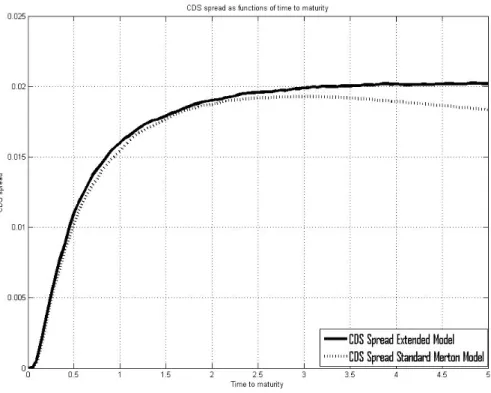
Figures (3), (4) and (5) plot the simulation results from both the standard Merton (1974) model and the proposed model. The results appear as expected. Theory suggests that the risk premium should increase due to the increased level of uncertainty. From figure (4), it is visible that the predicted CDS term structure is higher for the extended model than for the standard Merton model. The increase is, however, quite small, perhaps smaller than one would suspect. The difference between the predictions from the two models is larger as the time to maturity increases. This is as expected, because the uncertainty will become more significant at longer time horizons. But even five years into the future, the predicted CDS spread is only roughly 2 basis points (bp) higher than the one obtained from the standard Merton model. The probability of default plotted in figure (5) shows the reason behind the small increase. The probability of default is only increased by about 3 percentage points at its highest. The expected payoff on the CDS is thus merely marginally higher than what is predicted by the standard Merton model. As a consequence, the CDS is required to have a slightly higher spread in the extended model in order to avoid arbitrage

Figure 3: Comparison of the Simulated Credit Spread From the Standard and the Ex-tended Model

(37)

Figure 4: Comparison of the Simulated CDS Spread From the Standard and the Extended Model

Figure 5: Comparison of the Simulated Default Probabilities From the Standard and the Extended Model

(38)

An interesting feature of moving from the standard model to the extended one, is that the credit spread on the underlying bond increases by much more than the CDS spread. The simulated value from the extended model is more than twice the size of the value simulated with the standard Merton model for a large part of the time period investigated. There could be a number of reasons why this is happening. As is clear from figure (3), the standard Merton model predicts a humpback shaped term structure, while the extended model predicts an upward sloping term structure for the calibration considered. The humpback shape is a well documented phenomenon in structural models when dealing with low quality bonds (Agrawal & Bohn, 2005). The shape arises from several reasons, but most significantly it is due to the underlying distribution of default probabilities. The extended model does not have the same humpback shape in figure (3). As discussed by Agrawal & Bohn (2005), the Collin-Dufresne & Goldstein (2001) variant of the Merton (1974) model with a stationary leverage ratio does not necessarily predict term structures with the same shape as the original Merton model. Depending on the parameters, different shapes can occur for similar bonds depending on which of the two models is used. This seems to be the case here, as the extended model is clearly upward sloping. The different shapes of the term structures cause the increase in predictions for long maturities to be relatively large. This increase can also here be explained by increased uncertainty, and hence increased risk.

One interesting feature of the calibration of the extended model is that the debt target level is set to a lower value than the debt starting value. This would imply that the company will seek to reduce the debt level relative to the start value. The ceteris paribus effect of this would be a lower probability of default, and hence a lower risk premium. Although this effect is probably pulling down the CDS spread, it is not enough to offset the effect of the increased risk caused by the other extensions. This could very well serve as a possible explanation as to why the simulated CDS spreads are not higher in the extended model. At the same time, the long term volatility rate is calibrated to be higher than its start value, creating a similar effect as the mean reverting debt, but in the opposite direction. Changes in these parameters are investigated further in the sensitivity analysis (see chapter 5.4).

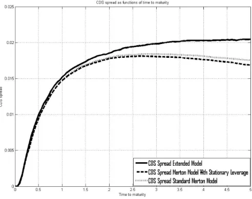
It is interesting to see how much of the change in the simulated term structure is caused by the new extensions suggested in this thesis. Figure (6) compares the simulated CDS spread for the calibrated parameters using a) the standard Merton (1974) model, b) the stationary leverage version, as suggested by Collin-Dufresne & Goldstein (2001), and c) the model suggested in this thesis.

(39)

Figure 6: Comparison of the Simulated CDS Spread From the Standard Merton Model, the Merton model With Stationary Leverage and the New Model Proposed in This Thesis

Figure 7: Comparison of the Simulated CDS Spread From the Standard Merton Model, the Merton model With Stationary Leverage and the New Model Proposed in This Thesis. Initial debt value is set below the debt target level: D= 0.5, Dtarget _{= 0}_.₆

(40)

A striking result is that the model with a stationary leverage, but no other extensions, actually lowers the simulated CDS term structure. As discussed above, this could be the result of a debt value today that is above the target level. If the debt level today is set to a lower value than the target level as in figure (7), the simulated spread is larger than what is predicted by the standard Merton model. It seems that the other extensions made to the model significantly increase the simulated CDS spread. The debt process can cause both an increase and a decrease in the spread, depending on the model calibration. Also worth noting is the signs of downward sloping curves at long maturities for the Merton and Collin-Dufresne & Goldstein models, consistent with the discussed humpback shape. The general conclusion is that the extended model produces higher term structures for CDS contracts with the current calibration.

5.4 Sensitivity Analysis

In order to fully understand the dynamics of the new model, it is useful to conduct a sensitivity analysis. The sensitivity analysis investigates the effect of each parameter in the model by changing the input values. The goal of this section is to see how the extended model reacts when economic conditions change, and if it is more or less sensitive to such changes than the standard Merton (1974) model. The sensitivity analysis is carried out by changing one parameter at the time while holding all other parameters constant at the calibrated level. Each parameter is both increased and decreased to investigate how it is affecting the predicted CDS spread.

The sensitivity analysis investigates ceteris paribus effects only. This does not always give the correct picture of the real world dynamics, as some of the input parameters arguably can be correlated with each other. As an example, it is possible that the debt and the expected growth rate are somehow related. Up and coming companies may issue a lot of debt relative to firm value today because they expect to grow in the future. This way the growth can finance the repayment of their liabilities. Large, established companies, on the other hand, may have to be more careful when issuing debt as they can not rely on future growth to finance the debt repayment. If this is the case, the full effect of the correlated change in debt and growth rate is not picked up by this analysis. On the other hand, the directional change from each parameter alteration should give a hint as to what will happen even in the case of correlated input values.

(41)

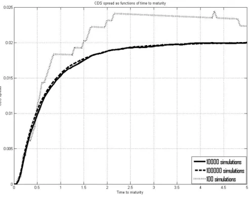
5.4.1 The Number of Simulations: Nsim

Increasing the number of simulations for each time step will give better approximations and produce a smoother looking curve. The effect of increasing the number of simulations beyond 10,000, however, is quite small. Simulations of 100,000 times 100 time steps have been conducted. This increases the computational time dramatically (see appendix A.1 for specifications of the computer used). As figure (8) shows, the approximations appear to be equally good for 10,000 and 100,000 simulations per time step. It thus seems unnecessary to do any more than 10,000 simulations. Reducing the number of simulations makes the simulated curves very uneven, and give quite rough estimates. Figure (8) also shows the results from reducing the number of simulations to 100 per time step. These results deviate quite substantially from the other two simulations. This is a direct result of the central limit theorem: as the number of simulations are increased, the average value will approach its real value. At a certain point the approximations get so close to the “true” value that increasing the number of simulations will only have a negligible effect. A differing number of simulations require a differing number of random variables. The three simulations in figure (8) have been conducted using different computer generated random numbers, but the results from the 10,000 and the 100,000 simulations are still hard to separate. This is the central limit theorem in practice. When the number of simulations are reduced to 100, there are not enough observations to eliminate the extreme values.

(42)

In the particular case of figure (8), the results seem to be overstated when using too few observations.

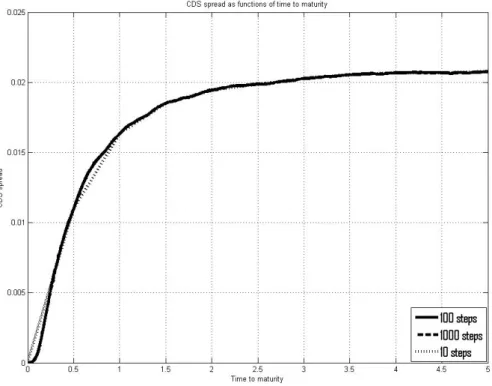
5.4.2 The Number of Time Steps: N

A higher number of time steps will decrease the length of each step for a given time to maturity, giving a better approximation to the assumed continuous time framework. Figure (9) shows that the number of steps does not have any significant impact on the shape of the CDS term structure. 100 or 1,000 steps seem equally suited for the task. If

N is reduced to 10 steps, it still approximates the continuous variable fairly well, although the graph is slightly less smooth. The difference between the three simulations are hard to separate in figure (9), but the simulation with only 10 time steps stands out as less compelling than the other two. The results from the simulated bond spread and the probability of default share the same story of little or no impact occurring due to changes in the number of time steps.