Distributed on-line dynamic task assignment for multi-robot patrolling

(will be inserted by the editor)

Distributed On-Line Dynamic Task Assignment for

Multi-Robot Patrolling

Alessandro Farinelli · Luca Iocchi · Daniele Nardi

Received: date / Accepted: date

Abstract Multi-Robot Patrolling is a key feature for various applications related to surveillance and security, and it has been studied from several different perspectives, ranging from techniques that devise optimal off-line strategies to implemented sys-tems. However, still few approaches consider on-line decision techniques that can cope with uncertainty and non-determinism in robot behaviors.

In this article we address on-line coordination, by casting the multi-robot pa-trolling problem as a task assignment problem and proposing two solution tech-niques: DTA-Greedy, which is a baseline greedy approach, and DTAP, which is based on sequential single-item auctions. We evaluate the performance of our system in a realistic simulation environment (built with ROS and stage) as well as on real robotic platforms. In particular, in the simulated environment we compare our task assign-ment approaches with previous off-line and on-line methods. Our results confirm that on-line coordination approaches improve the performance of the multi-robot pa-trolling system in real environments, and that coordination approaches that employ more informed coordination protocols (e.g., DTAP) achieve better performances with respect to state-of-the-art online approaches (e.g., SEBS) in scenarios where interfer-ences among robots are likely to occur. Moreover, the deployment on real platforms (three Turtlebots in an office environment) shows that our on-line approaches can successfully coordinate the robots achieving good patrolling behaviors when facing

Alessandro Farinelli

Department of Computer Science University of Verona, Italy E-mail: [email protected] Luca Iocchi

Dept. of Computer Control and Management Engineering Sapienza University of Rome, Italy

E-mail: [email protected] Daniele Nardi

Dept. of Computer Control and Management Engineering Sapienza University of Rome, Italy

typical uncertainty and noise (e.g., localization and navigation errors) associated to real platforms.

Keywords Multi-robot patrolling·Distributed Multi-Robot Coordination·Dynamic Task Assignment

1 Introduction

Patrolling, that is the continuous monitoring of an environment, is an important activ-ity for applications related to securactiv-ity and surveillance; using multiple robots for pa-trolling clearly helps improving task performance. Therefore,Multi-robot patrolling (MRP) is a problem that has been studied from many different perspectives in the last years, including formal representations of the problem, optimal solutions, theoretical analyses, implementation and experimental validation.

Although a relative large literature on this topic is available, experiments on real robots or on realistic simulators are rather limited. With some notable exceptions (see next section), most previous approaches focus on defining patrolling strategies according to static characteristics of the environment (for example, the layout of the map) and of the robots, without taking into account problems arising in actual de-ployment of real robots in a real environment.

On the other hand, perception noise and non-deterministic effects of action ex-ecution, that cannot be avoided by robots acting in the real environment, are not modeled, while they significantly affect patrolling performance. In many cases, opti-mal strategies obtained in ideal situations are suboptiopti-mal (or they may even fail) in a real situation. In other cases, no static solutions with good performance can be found: for example, in environments that do not contain loops (thus cyclic patrolling is not possible or inconvenient because of interferences among robots) and that cannot be partitioned in a balanced way (thus making the work of some robots unbalanced with respect to the others). The work in [14] analyzes some of these situations and advo-cates the use of on-line patrolling approaches strategies to address those issues.

However, to devise and execute effective on-line MRP strategies, robots must be able to coordinate their movements while patrolling, so to optimize their choices by considering up-to-date information and hence cope with the inevitable effects of uncertainty in perception and action execution. Moreover, the use of decentralized coordination approaches is a key issue for the deployment of practical MRP systems. In contrast to centralized solutions, decentralized approaches do not have a single point of failure and offer more flexible implementations (e.g., they do not require all robots to be connected to a base station at all time).

In this article, we investigate decentralized on-line coordination approaches for multi-robot patrolling, and show that dynamic task assignment techniques can be successfully employed to coordinate robot actions in presence of non-modeled char-acteristics of the real environment. In more detail, the present article makes the fol-lowing contributions to the state of the art:

1. Formulation of the on-line coordination problem associated to MRP as a Dy-namic Task Assignment (DTA) problem; this allows to use state-of-art solution approaches for DTA to perform on-line coordination for MRP.

2. Description of two dynamic, decentralized task assignment solution techniques for MRP: a greedy baseline approach (DTA-Greedy) and a market-based ap-proach based on sequential single item auctions (DTAP); for the latter apap-proach, we present a novel bidding strategy that departs from standard rules (such as min, avg or max path cost [27]) and is based on a dynamic partitioning of visit loca-tions that are all close to each other, hence minimizing the possible interferences among robots.

3. Critical analysis of the performance metrics for measuring performance of on-line MRP solutions. In particular, we show that an evaluation of the methods based only on standard metrics, such as global idleness average, global idleness standard deviation and global maximum idleness, might not provide enough information to allow for a suitable comparison of different methods. Hence we propose novel forms of representing the results of a MRP task that allow for a more detailed analysis of the MRP performance.

4. Evaluation of the proposed techniques and comparison with previous methods in a realistic simulation environment for multi-robot patrolling,patrolling sim1, that is based on ROS and Stage. Moreover, an implementation of the developed algorithms has been also tested in a real environment with three Turtlebots. The experiments show that on-line coordination is crucial to improve system per-formance with respect to static patrolling strategies and non-coordinated dynamic choices. Specifically, our decentralized coordination methods provide good patrolling solutions and adjust to unpredictable changes in the patrolling team (i.e., due to robot malfunctioning/failures). Moreover, we usedpatrolling simto perform a quanti-tative comparison of our proposed approaches with several state of the art techniques [19], considering both on-line and off-line approaches in several experimental set-tings (i.e., varying the number of patrolling robots and the floor maps). Our results, show that on-line coordination is needed to provide an effective patrolling system, and that the market-based coordination method we propose has many advantages over the other on-line coordination approaches we considered.

The rest of the paper is organized as follows: Section 2 puts our work in per-spective with previous approaches for patrolling. Section 3 defines the on-line Multi-Robot Patrolling (MRP) problem we address. Section 4 provides a formulation of the on-line MRP problem as a Dynamic Task Assignment problem and proposes two DTA techniques: DTA-Greedy and DTAP. Section 5 describes the performance met-rics and the experimental evaluation of the proposed approach. Finally, Section 6 concludes the article.

2 Related Work

The literature on MRP shows a significant body of work on the problem and pro-vides a wide ranges of solution techniques. To better frame our approach with respect

1 _{The simulator was originally developed by David Portugal and has been used to compare patrolling}

strategies in previous work (e.g., [22]). We modified the simulator to include our DTA approaches and to improve the behaviours of the robots for providing more realistic simulations. The current version of the

to the current literature, we consider three main dimensions that characterize most important algorithmic aspects of previous work in this area: i) adversarial vs. non-adversarial approaches; ii) continuous vs. discrete environment representation; iii) on-line vs. off-line solutions.

Adversarial approaches (also called strategic approaches), such as [1] or [6], con-sider and explicitly model the presence of an intruder trying to find the best strategy to enter the system and typically formulate the patrolling problem using game-theoretic concepts. On the other hand, non-adversarial approaches do not model the presence of an intruder and are typically used for applications such as environmental monitoring or rescue operations [26], or where no information about the intruder are available or no assumptions are made. Here we consider the non-adversarial application scenar-ios, hence we do not further discuss the literature pertaining to adversarial patrolling. Several works focus on patrolling in continuous areas [11, 4, 3, 16], where pa-trolling metrics (e.g., idleness) must be considered at every point of the environment. In contrast, other approaches such as [5, 9, 20, 22] focus on a discrete representation of the environment that typically takes the form of a patrol graph, where nodes repre-sent specific locations that the agents have to travel across and, typically, no assump-tions are made on the properties of nodes or regions to be patrolled. In this work, we adopt the graph-based representation, since it allows to add a-priori information about which locations must be visited in an environment. Notice that, in the solutions using patrol graph, interferences between robots are typically considered only on the patrol nodes (i.e., when robots visit the same node of the graph). In contrast interferences that might occur on the edges (i.e., when robots are traveling between visit locations) are typically ignored. In our work, although using a graph-based representation, we provide an algorithm (DTAP) that aims at reducing also the number of interferences on the edges.

Off-line solutions [11, 20] pre-compute paths that robots must follow before mis-sion execution, while on-line solutions [19, 22, 25, 4, 18] compute (or modify) paths while robots are patrolling. On-line solutions can use most up-to-date information and hence compensate for non-modelled characteristics of the environment. On the other hand, off-line solutions typically provide optimal or near-optimal guarantees on solution quality.

Many off-line approaches model MRP through a patrol graph [15], thus allowing to apply several results from Graph Theory. Several strategies have been proposed to navigate the resulting path. Among them, graph partitioning (e.g., [20, 26]) is often used as a basis for comparison. This comparison is performed using different met-rics that have been suggested for determining the optimal solution:idleness ([9]), frequency2([10, 11]) orexploration time([15]).

However, the theoretical analysis developed on graphs is typically based on rather unrealistic assumptions on the operational environments and on the behaviour of the robots. Consequently, recent research focuses on experiments with real robots or with realistic simulators, where both the features of the environment and the robot capa-bilities (e.g. localization, navigation, communication and perception) are taken into account. For example, Portugal and Rocha [21] and Iocchi et al. [14] use a realistic

simulator, based on a ROS implementation, while Agmon et al. [3] developed an in-teresting simulator that includes a model of environmental conditions (i.e., currents in a maritime scenario). Few experiments with real robots have also been performed: Elmaliach et al. [12] use a team of 3 modified vacuum cleaners to show the impact of velocity uncertainty in the motion model; Marino et al. [17] use a team of 3 Pio-neer robots to patrol the perimeter of a predefined area. Recently, extending previous work, Portugal and Rocha [23] present an analysis on five different algorithms using a realistic simulator as well as experiments with five Pioneer robots.

The more realistic validations of MRP approaches show that the theoretical strate-gies need to be adapted to take into account the uncertainties and dynamics of the ac-tual execution and, more generally, on-line coordination techniques are needed. Con-sequently, alternative approaches have been proposed, based on reinforcement learn-ing [24], on multi-agent Markov decision processes [16], or uslearn-ing Bayesian learnlearn-ing [19].

In this paper, we develop an on-line task assignment approach to increase the ro-bustness of MRP when dealing with the uncertainties arising from action execution in a real environment. Specifically, we propose to model on-line MRP as a dynamic task assignment problem, thus providing a general framework for on-line coordination of MRP. On-line MRP shares similarities with approaches for on-line multi-robot ex-ploration, where robots cooperatively choose the next frontiers to visit aiming at op-timizing the information acquisition process [13, 8]. However, in on-line MRP, robots must visit locations repeatedly minimizing the idleness rather than acquiring new in-formation on the environment. This results in important differences in the employed coordination strategies. An early work considering on-line MRP is the one by Semp´e and Drogoul [25], who address MRP by dynamically assigning tasks to robots. Task data are propagated through a centralized virtual world, and robots follow the gra-dient determined by the task strengths. Robustness to communication failures has been considered in [2], where authors empirically evaluate on real platforms differ-ent patrolling strategies with varying levels of coordination (no coordination, loose coordination and tight coordination). More closely related to our approach is the work by Ahmadi and Stone [4], where a negotiation is proposed to dynamically assign the frontier cells to be visited by the robot that has more time available. In fact, this work is very similar in spirit to our proposal. However, major differences with re-spect to our approach are that Ahmadi and Stone assume that robots start-off from a pre-computed partitioning of the cells, and that robots can negotiate only on frontier cells. In contrast, in our work, robots start-off with no pre-computed allocation and build a partitioning entirely through negotiation (which can involve any visit loca-tion). While using a pre-computed partitioning might be beneficial for some aspects (e.g., it would immediately provide the robots with a good allocation) such a solu-tion might require more time to react to unexpected changes in the environment (e.g., when a robot exits/enters the system). Finally, the approach by Ahmadi and Stone is designed for a grid representation of the environment and should be adapted to work on a graph representation, that is more common in previous works. Recently, Pippin et al. [18] provide an approach to monitor robot performance in a multi-robot pa-trolling system (using a centralized computational unit) and to re-assign tasks when robots perform poorly. Task re-assignment is performed by using an auction-based

method where poor performing robots auctioff their tasks. We also consider on-line coordination and propose a market-based technique, but in our approach robots continuously negotiate over all available tasks. Moreover, we developed a completely decentralized system that can immediately react to unexpected changes (i.e., a robot that leaves or enters the system).

3 Problem Definition

In this section we define the MRP problem considered in this article. A set of robots R={r1, ...,rn} act in a known environment with the objective of visiting all the relevant places as often as possible. The environment in which the robots act is repre-sented as apatrol graph PG=<P,E,c>, wherePis a set ofpatrol nodes, i.e. poses (position and orientation) in the environment that the robots have to reach to take some observation,E⊆P×Pis a set of edges connecting the nodes,cis a function denoting the expected travel time for each edge.

The MRP problem can be solvedoff-line, by defining the pathsπibefore the MRP task starts, oron-line, by building such paths during the MRP task execution. On-line solutions to the MRP problem dynamically choose a pathπi=hp1, ...,pti, for each robotriso to maximize the MRP performance. These solutions are characterized by the fact that each robot updates its path, while patrolling, by considering information on the current performance of the system. Coordinated on-line solutions are also characterized by explicit negotiation among robots.

Standard performance measures for MRP are based on theidlenessof the nodes [15]. The instantaneous idleness Ip(t) for a node p at timet is the elapsed time since the last visit from any robot in the team. Letht0,t1, ...,tkibe the time frames in which any robot of the team visitsp, then we can collect the idlenesses of nodep ashIp(t1), ...,Ip(tk)i(i.e.,Ip(tj) =tj−tj−1). From these values we can calculate the

average idlenessof a nodeIavgp and itsstandard deviation I_stddevp . Finally, three global measures can be computed by determining average, standard deviation and maximum of all the valuesIp_{(t)for every timet and everyp∈P. We refer to these measures} asglobal idleness average IG

avg,global idleness standard deviation IstddevG , andglobal maximum idleness I_maxG , respectively.I_stddevG actually measures how balnaced are the visits to the nodes: low values forI_stddevG mean that all the patrol nodes are visited approximately with the same frequency. WhileIG

maxrepresents a worst case analysis. From these definitions, different performance metrics may be considered for eval-uating the performance of a MRP system. A typical choice is to minimize the global idleness average, which is in general a good measure. However, in some cases, a good average can be obtained with a large standard deviation, meaning that some nodes are visited very often and some other nodes are visited less often. This may be unacceptable for some surveillance applications. On the other hand, it is possible to minimize the global idleness standard deviation, thus guaranteeing a more uniform visit of all the nodes, but this may be in contrast with minimizing the global average idleness. Thus, a trade-off between global idleness average and global idleness stan-dard deviation should be considered, as it may better characterize the overal system performance. Moreover, specific needs of the application scenario may lead to prefer

some performance metric over the others. Section 5.3 provides more details about the analysis of MRP performance.

In the following, we will use the termMRP performanceto refer to any perfor-mance metric based on the concept of idleness that is defined by the designer of the surveillance application.

4 Dynamic Task Assignment for on-line MRP

In this section we describe how to employ Dynamic Task Assignment (DTA) for developing on-line solutions for the MRP problem.

The MRP problem, as defined in the previous section, is characterized by a set of robotsR={r1, ...,rn}, a patrol graphPG=<P,E,c>, and some MRP performance metrics. The goal of the multi-robot system is to choose a pathπi=hp1, ...,pti, for each robotri, so to maximize such MRP performance metrics.

The DTA problem associated to MRP consists of a set of tasksT ={τ1,· · ·,τm}a set of robotsR={r1,· · ·,rn}and a reward matrixV={vi j}, where eachvi jindicates

the reward the system achieves when robotriexecutes taskτj. An allocation matrix

A={ai j}defines the allocation of robots to tasks, withai j∈ {0,1}andai j=1 if and only if robotriis allocated to taskτj. The goal of the system is then to find the best assignment of tasks to robots with respect to the given reward, i.e.

A∗=arg max A |R|

∑

∑

Moreover, a set of constraintsC usually describes valid allocations of robots to tasks (e.g., one task per agent) and hence the above optimization must be performed subject toC.

In our patrolling problem, tasks are locations to be visited, i.e., a set of patrol nodesP={p1,· · ·,pm}and rewards depend on the average idleness of a node and

on the travel cost that a robot incurs to visit such node. Specifically, we have that vi j=U(ri,pj,t), whereU(ri,pj,t)is a utility function that encodes how good is for the system to allocate robotri to node pj at current timet. An example of such a utility function may be

U(ri,pj,t) =θ1Ipj(t) +θ2T c(ri,pj,t)

whereIpj_{(t)is the idleness of p}

j at timet,T c(ri,pj,t)is the travel cost for robot rito reach pjconsidering the robot position at timet, andθ1,θ2are parameters that

balance travel cost and idleness. Moreover, we enforce the constraint that, at any timet, only one robot should be allocated to a specific location (i.e.,∀t,j∑iai j≤1) to maintain a similar visit frequency across the locations.

Notice that, in our DTA problem the costs and the allocation matrices depend on time; however, as it is frequently the case in the task assignment literature, we actually solve a one shot allocation and then iterate the decision process over time.

Furthermore, notice that, our formalization of the DTA problem does not explic-itly represent paths for the robots (i.e., a task is one patrol node and not a sequence of

such nodes), hence at each time step only a subset of the tasks might be allocated (this depends on the solution approach as described below). However, over time robots effectively build paths that visit patrol locations based on the current value of the idleness.

In what follows, we detail two methods for Dynamic Task Assignment: DTA-Greedy and DTAP. Both methods provide a form of distributed coordination based on explicit communication. The difference between these two methods lies in the coordination protocol and on the length of the path that robots consider. In particu-lar, DTA-Greedy can be considered as a baseline, while DTAP is a more informed method for solving on-line MRP with DTA. In fact, in DTAP robots negotiate over all patrol nodes to build a partition of visit locations over the robots, while in DTA-Greedy they negotiate only their next patrol node and aim at avoiding conflicts (e.g., two robots heading towards the same target). In other words, DTAP allocates a subset of patrol nodes to each robot (i.e.,∀i∑jai j≥1), hence considering the paths that robots will follow, while DTA-Greedy always allocates one patrol node to each robot (i.e.,∀i∑jai j=1). By considering and exchanging more information, DTAP takes better decisions and, hence has better performance (see Section 5).

4.1 Shared representation of information

The algorithms described in this section are totally distributed and thus each robot has a local representation of the information, that is an estimate of the unknown global state of the world.

Each robotrk maintains a local copy of the instantaneous idlenesses of all the nodes, denoted byIP_(t)(rk)_=hIp1_{(t), ...,I}pn_(t)i(rk)_{. As mentioned above, these}

idle-ness values do not correspond in general to the actual idleidle-ness of the MRP task and they may be different for each robot (unless communication is broadcast and instan-taneous).

The robots periodically exchange and integrate information about their status and the information sent by every robot include its local estimates of the idlenesses.

The algorithms are based on events and a new decision about the patrol path is taken when one of these two events occur: (1) the robot reaches its current target node, (2) the robot receives a message from another robot. Note that, after deciding the initial target with any method (e.g., the closest one), the first event will eventually occur. The following notation is used:rkis the robot running the algorithm;Pis the set of patrol nodes,IP(t)(rk)_{is a vector of instantaneous idleness of all the nodes for}

robotrk, withIP(0)(rk)=h0, ...,0i; pk is the current target node for robotrk;tk is the last update time ofIP(tk)(rk);tis the current time when the algorithm is running; IP(t)(rj)_andp

jare the instantaneous idlenesses and the current target node of robot rjas received by robotrk; finally,p∗is the next target node forrk.

The algorithms presented in this section assume normal operations of the robots (i.e., no major failures occurring). This means, for example, that if a robot aims at reaching a target, it will eventually reach it. Dealing with major failures is not ex-plicitly considered by the following algorithms. Some of these major failures (e.g., a

dead robot) are implicitly considered by the fact that the solution is on-line, and thus remaining robots will eventually reconfigure to take the tasks of the dead one.

4.2 Basic Dynamic Task Assignment (DTA-Greedy)

The first algorithm presented here is a basic DTA that performs a greedy maximiza-tion of the utility funcmaximiza-tionU(rk,p0,t). Decisions are taken by considering the local instantaneous idlenesses and the instantaneous idlenesses received from the other robots. The process is described in more detail in Algorithm 1, which is split in two parts corresponding to the two events to be handled.

Algorithm 1:DTA-Greedy 1 Eventnodepkreached:

2 Ipk_(t)(rk)_←0; 3 foreachp0∈P,p06=pkdo 4 Ip0(t)(rk)_←Ip0_(t k)(rk)+ (t−tk); 5 p∗←argmax_p0U(rk,p0,t); 6 Ip∗_(t)(rk)_←0; 7 send(<IP(t)(rk)_,p∗_>); 8 tk←t; 9 gotoTarget(p∗); 10 11 Event<IP(t)(rj)_,p

j>received from robotrj:

12 foreachp0∈Pdo 13 Ip0(tk)(rk)←min(Ip 0 (t)(rk)_{+ (t−t} k),Ip 0 (t)(rj)_); 14 tk←t; 15 ifpj=p∗then 16 p∗←argmaxp0U(rk,p0,t); 17 gotoTarget(p∗); 18 send(<IP_(t)(rk)_,p∗_>);

When a target node is reached [lines 1–9],IP(t)is updated accordingly and then the next target node p∗ is chosen by maximizing the utility function. The value of Ip∗_{(t)is also set to 0, so that the utility function for this node will decrease for the} other robots, thus trying to avoid conflicts in accessing the same node.

When idlenesses of another robot are received [lines 11–18], the local values ofIP(t)(rk) _{are updated with the minimum between the received valueI}p0_(t)(rj) _and

the current estimates as known byr_k,Ip0_(t

k)(rk)+ (t−tk). Notice that this update rule assumes (lacking any knowledge about it) that all the other robots have not visited any other nodes meanwhile. Furthermore, notice that the algorithm updates the idleness of all the patrol nodes in P, even though the message received from robotrj relates to a specific nodepj. Now, under the assumption of perfect communication and no robot failure this is redundant, as each robot could update only the idleness of node pj. However, when messages can be lost, or when robots can enter the system during

the patrolling mission, such redundancy helps robots to quickly reach a common estimate for the idleness of all patrol nodes. Next, if a conflict is detected (i.e., the current target node for robotrkequals the target node of robotrj), a new target p∗is computed by maximizing the utility function. This means that a robot can change its destination during its path towards a node. This can happen when a realistic or a real model for communication is used (as in the simulation experiments described in this article and with real robots), in which non-instantanous messages3may result in two robots choosing to go to the same target node.

In DTA-Greedy algorithm, we have used the following utility function

U(rk,p0,t) =θ1Ip

0

(t) +θ2T c(rk,p0,t) +θ3d0(rk,p0)

where, in addition to the termsIpj_{(t)andT c(r}

i,pj,t)defined before, we also consider the distance d0(rk,p0) between the node p0 to be reached and the initial node for robotrk(i.e., the very first node in whichrkwas when the MRP task started). This special heuristic is suitable when robots start the task in a distributed fashion (i.e., from distant locations each other) and this term of the utility function tends to keep the robots apart from each other to avoid interferences. More in general, heuristics to spread out robots have been frequently employed in multi-robot coverage [7] and exploration [8].

Of course other heuristic functions can be defined, for example, functions that are specific of the environment. The definition of a proper heuristic is not the focus of this article, since DTA-Greedy is only shown here as a baseline of a simple method based on DTA. Furthermore, good performance of this utility function depends also on a proper set-up of the parametersθi. In this work, no optimization of these pa-rameters has been performed and the same set of papa-rameters has been used in all the experiments.

4.3 DTA based on Sequential Single Item Auctions (DTAP)

DTAP is inspired by auction based task allocation: the basic idea is that robots an-nounce their destinations to everyone and then collect “bids” from their team-mates. Such bids encode how well each robot fits to a given destination. In more detail, each robot selects the next visit node as the one that maximizes a utility function. Then the robot broadcasts its node selection, announcing its corresponding bid, to all team mates. After collecting all bids the robot checks whether it is the one with the best bid for the selected node. If this is the case, the robot visits the selected node, otherwise it selects the next best visit node and iterates the selection process.

Our market based allocation scheme takes inspiration from Sequential Single Item auctions, where robots allocate one task at the time, and when they compute their bids, they consider previous allocated tasks. This allows to take into account important synergies between tasks (i.e., patrol nodes that are close to each other). In our approach, such bid computation considers the number of tasks a robot is respon-sible for and the distance of the target node to thecentral node, which is the node

Algorithm 2:DTAP 1 Initialization:

2 CurrentTasks←P; // Initialize CurrentTasks with all patrol nodes

3 MyTasks←/0 ; // Initialize MyTasks with the empty set

4

5 Eventnodepkreached:

/* Update Idleness of all patrol nodes */

6 Ipk_(t)(rk)_←0;

7 foreachp0∈P,p06=pkdo

8 Ip0_(t)(rk)_←Ip0_(t

k)(rk)+ (t−tk);

9 tk←t; // update last visit time with current time

10 p∗←argmaxp0_{∈CurrentTasks}U(rk,p0,t); // select best node amongCurrentTasks

11 CurrentTasks←CurrentTasks\p∗; // remove selected node fromCurrentTasks

12 bid←computeBid(p∗); // compute bid for p∗

13 f orceBid(p∗,bid,ri); // assume this robot is the best one to patrol p∗

14 sendTarget(p∗,bid); // send target and bid to other robots

15 collectAllBids();// wait for bids from other robots (this inlcudes a timeout) /* check whether this robot has the lowest bid */

16 ifbestBid(p∗)then

17 CurrentTasks←P; // reset CurrentTasks

18 MyTasks←p∗; // allocate this robot to p∗

19 pnext←chooseNextNode(MyTasks); // choose the best task to patrol

20 gotoTarget(pnext); // go to pnext

/* check if there are still tasks the robot should consider */

21 else ifCurrentTasks==/0then

22 CurrentTasks←P; // reset CurrentTasks

23

24 Eventmsgreceived from robotrj:

25 ifmgs.type==IPthen

/* Update Idleness of all patrol nodes */

26 foreachp0∈Pdo 27 Ip0(tk)(rk)←min(Ip 0 (t)(rk)_{+ (t−t} k),Ip 0 (t)(rj)_);

28 tk←t; // update last visit time with current time

29 else ifmsg.type==Bidthen

/* Maintain best bid for each patrol node, update MyTasks so to include nodes for which this robot has lowest bid */

30 updateBids(msg.dst,msg.value,msg.sender);

31 updateMyTasks()

32 else ifmsg.type==Targetthen

/* Handle task request */

33 bid←computeBid(msg.dst); // compute bid for the target

34 updateBids(msg.dst,msg.value,msg.sender);

35 updateMyTasks();

/* Check whether the bid of this robot is better */

36 ifmsg.value>bidthen

at minimum path distance from all other nodes (see below for a more detailed ex-planation). This is different with respect to standard bid computation rules employed in sequential single item auctions for task allocation (e.g., [27]), that typically con-sider an aggregation of the path cost to cover all allocated tasks (e.g., the sum, max or average of the path cost). The rational behind this choice is twofold: i) by consid-ering the number of nodes, we foster a balanced workload among the robots and ii) by considering the distance to thecentral node, we aim at creating a partition of the patrol nodes that tries to minimise path crossing among the robots, hence resulting in less interferences for navigation. Moreover, we do not consider marginal costs for bid computation, as this could result in unbalanced allocations (as stated in [18]), where some robots might have significantly more visit nodes than others. This would be problematic for the MRP strategy as it would increase the standard deviation of the global idleness.

Our DTAP approach is described in Algorithm 2, which is again split in two parts corresponding to the two events to be handled. Whenever a robot completes a task (i.e., it reaches its current destination) [lines 5–22], it selects the next destination (p∗) as the one that maximises the utility function. Next, the robot computes its fitness for this destination (bid), and sends a target request (sendTarget(p∗,bid)) to all the robots.

After announcing its next target, the robot waits to receive the bids from the other members for that target (collectAllBids()); this function is blocking and a time out is used to avoid deadlocks due to possible robot failures. Notice that, waiting for a specified amount of time whenever a decision must be made, can significantly slow down the patrolling operations, hence resulting in a higher average idleness. However, this can be avoided by reasoning in advance on the future destination. In particular, robots can select the next destination, while travelling to the current target. Hence the waiting time for bids is absorbed by the travelling time to the current destination. Our current implementation employs this scheme, however, for ease of explanation, the pseudocode reported here assumes that each robot always chooses its next target after the current goal is completed.

After collecting all the bids, the robot checks whether its own bid is the best one for node p∗, if this is the case, it selects the best destination among its tasks (chooseNextNode(MyTasks)) and goes towards this destination. Moreover, it resets the task list, as appropriate [lines 16–20]. The choice of the next position (pnext) should try to maximize the system performance considering all the nodes that the robot should patrol, this requires to solve a problem that in general is not tractable as it reduces to a TSP. However, in our implementation we observed that a good and simple heuristic is to always choose the patrol node with the highest utility among the robot’s tasks, hence in practice this amounts to simply setpnext=p∗.

When a message is received by another robot [lines 24–37], first the local values ofIp0(tk)(rk)are updated as explained for DTA-Greedy .

If the message is abid(i.e., a robot is responding to a previous task request issued by this robot), the bids are updated (updateBids(msg.dst,msg.value,msg.sender)) so to always maintain the lowest bid for each patrol node. Once bids are updated the robot updates its tasks (updateMyTasks()) by modifying the structureMyTasksso to include nodes for which the robot holds the lowest bid.

If the message is a task request (i.e., this robot must respond to a task request of the sender), the bid of the current robot for the target is computed and sent to the message sender. Notice that, the robot communicates its bid only if it isusefulfor the sender, i.e., if the computed bid is lower than the one communicated (this reduces the number of messages for the coordination).

In order to effectively deploy sequential auctions a number of additional issues need to be suitably addressed and they are discussed below. First, the possibility that robots disappear during mission execution must be considered: if the best robot to perform a taskti is a robotrj and such robot disappears, the taskti will never be executed unless someone else becomes best suited for that task, which might never happen. This is addressed when choosing the next target position after computing the best candidate node, by the f orceBid(dst,value,sender)function, which forces the current bid as the best one. Moreover, the next node to reach is selected independently of the tasks that the robot is responsible for [see line 10], hence if a robot disappears the task it was responsible for will eventually be considered by the others.

Another critical issue is the computation of a bidb(computeBid(dst)). As men-tioned before, our approach is based on the concept ofcentral node, which is the node that has minimum travel cost from all other nodes the robot is currently responsible for. In more detail, we compute the central node as follows:

cn=minp∈MyTasks

_∑

T c(p,p0)

whereT c(p,p0)is the travel cost from locationp to locationp0. In our implemen-tation, the travel cost is comuputed as the length (i.e., the number of edges) of the shortest path between the two nodes. The central node is updated each time the MyTasks structure changes (i.e., when the robot acquires or loses a task). Next, we compute the bid for a destinationdst by multiplying the number of tasks the robot is responsible for by the travel cost from the central node to the destination: b=|MyTasks| ∗T c(cn,dst). This computation of the bid helps balancing the work-load, as it penalizes robots that are responsible for too many tasks, and it considers synergies among tasks, by penalizing robots that have a central node which is far from the current destination. Notice that, a standard metric, such as for example the sum of travel cost for a tour that covers all tasks, would also achieve workload bal-ance; however, since the bid is not related to a central node, this metric would not facilitate space partitioning. As a result, it can produce several path intersections that can increase difficuty in robot navigation.

5 Experimental Setting and Evaluation

The goal of the experiments described here is to assess the performance of the pro-posed MRP algorithms in realistic scenarios. As already mentioned, in order to com-pare the performance of the different algorithms, we have usedpatrolling sim

simulator. The simulator has been modified for improving the behaviors of the robots and for providing more realistic simulations. In the simulations reported in this arti-cle, typical odometry and laser range finder noises are used, robots use the standard

ROS navigation stack (amclfor localization andmove basefor navigation), and exe-cute their tasks at a nominal maximum speed of 1.0 m/s. Moreover, as communication among robots is implemented through the use of ROS messages, but by introducing a fixed amount of delay of 0.2 sec in the exchange of each message. This simulates a typical delay when sending TCP packets on a wireless network as experienced in the experiments with real robots. Finally, we added the implementation of the DTA methods described in this paper, thus allowing for a full replicability of all the results reported in this section.

The use of the ROS framework allows for an easy porting of the developed meth-ods on actual robots, as described at the end of this section.

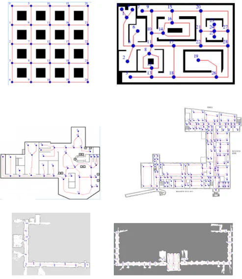
Fig. 1 Maps used in the experiments (not in scale): grid, example, cumberland, broughton, DIAG labs, DIAG floor1.

Map |P| |E| Size [m] grid 25 40 26×26 example 29 36 47×33 cumberland 40 44 52×37 broughton 163 186 100×80 DIAG labs 27 26 50×40 DIAG floor1 60 63 114×46

Table 1 Size of the patrol graphs used in the experiments.

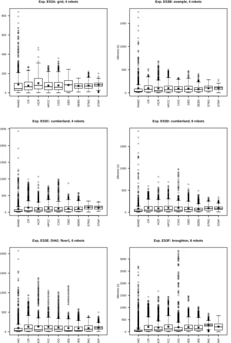
5.1 Evaluation scenarios and compared algorithms

Several different evaluation scenarios have been created in order to compare differ-ent algorithms in differdiffer-ent experimdiffer-ental conditions. Each scenario is defined by a map (see Figure 1) and the number of robots. Other variables of an experiment are discussed in Section 5.2.

The six maps used in the experiments are shown in Figure 1 and present different size and characteristics of the patrol graphs. Details on the number of nodes|P|, the number of edges|E|and the overall size of the area are shown in Table 5.1.

In the experimental evaluation reported in this article, the following algorithms have been compared:

– RAND - Random algorithm chooses the next vertex randomly among the adjacent ones.

– CR - Conscentious Reactive algorithm [15] selects the next node among the ad-jacent ones, based on its local estimate of the idleness.

– HCR - Heuristic Conscientious Reactive [5] is an extension of CR considering also the distance of the adjacent nodes from the current one.

– HPCC - Heuristic Pathfinder Cognitive Coordinated [5] considers path of length

>1 in the graph, instead of only the next adjacent node.

– CGG - Cyclic algorithm for generic graphs [9] is an off-line method computing Hamiltonian cycles (through a fast heuristic), when they exist, or long paths and non-Hamiltonian cycles.

– GBS - Greedy Bayesian Strategy [22] selects the next vertex to reach based on a Bayesian formulation of the problem for choosing the best direction. It uses information coming from other robots about their arrival time at a given node, so that a global idleness can be estimated.

– SEBS - State Exchange Bayesian Strategy [22] is an extension of GBS in which also intentions of other robots are collected and used for determining (again with a Bayesian method) the best direction.

– DTAG - DTA-Greedy algorithm described in this paper.

– DTAP - DTAP algorithm described in this paper.

The characteristics of the compared algorithms are also summarized in Table 2. On-line vs. off-line decision making is a first classification dimension. As already mentioned, on-line methods are more robust to non-modeled effects of the environ-ment, while off-line methods aim at optimizing the behavior of the robots given the prior knowledge about the environment. The path length determines how many nodes

Algorithm Decision Path length Communication RAND on-line 1 -CR on-line 1 -HCR on-line 1 -HPCC on-line >1 -CGG off-line >1 -GBS on-line 1 arrived

SEBS on-line 1 arrived + intention

DTAG on-line 1 utility values

DTAP on-line >1 two-steps protocol

Table 2 Summary of characteristics of the compared algorithms.

are planned to be visited at each decision. This is particularly interesting, of course, for on-line methods. In previous work, methods with path length 1 are called Re-active, while the others are called Cognitive. Finally, the table highlights the com-munication among robots, from no comcom-munication for non-coordinated methods, to minimum communication for methods with implicit coordination (GBS and SEBS) to explicit communication for methods based on a coordination protocol (DTAG and DTAP).

It is important to notice that the last four algorithms (GBS, SEBS, DTAG and DTAP) present some form of explicit coordination, based on communication of some information among the robots that are used to decide which path to select. In GBS, SEBS and DTAG, a single message is sent from a robot to all the others containing information that will be used to take decision. The content of the messages exchanged in SEBS and DTAG include some information about the intention of a robot to visit the next node. This feature (as shown by experimental results) allows for a significant reduction of the interferences. On the other hand, DTAP implements a two-steps co-ordination protocol, in which robots exchange information and negotiate their paths. Moreover, DTAP decision involves not only the next node to visit, but a subset of nodes. Therefore, DTAP implements a more informed coordination protocol with re-spect to the other methods.

For CR, HCR, HPCC, CGG, GBS and SEBS we have used the implementations available in patrolling simand we have added the implementation of RAND, DTAG and DTAP topatrolling sim. Other algorithms could be easily integrated and compared using this simulator in the future. Previous comparisons among these algorithms (except for DTA ones) are reported in [23] and [22]. Notice that values are different in this article since we are using a different setting for the robots (e.g., 1.0 m/s of maximum speed in the experiments reported in this article vs. 0.2 m/s used in previous experiments).

5.2 Variability of the experiments

The results of the experiments are mostly based on the concept of idleness, which de-pends on the time needed to reach nodes in the patrol graph and thus dede-pends on the underlying navigation module. Due to the choice of using a realistic simulator

mod-eling typical forms of uncertainty in mobile robots, someexternal factorsinfluence the results of the experiments, but are not part of the MRP algorithms. We believe that it is important to consider these factors in the experiments and not to hide them (by using for example a more abstract simulator or less noisy modules), since they are actually present in the real world.

In the following, we briefly describe and comment the most important external factors that affect the performance of MRP task.

1. Localization. Localization introduces some noise in the navigation component, but in our experience this noise does not affect the overall results of multi-robot patrolling in a significant way. Indeed, we consider robots equipped with a typical laser range finder navigating in an indoor environment with a known map. In this situation, standard localization methods based on particle filters (we use ROS

amcl) are known to be very robust and precise.

2. Path planning and trajectory following. The definition of the path to reach a target node and its execution also introduce noise, but also in this case standard implementations (we use ROS move base) are reliable enough and do not in-troduce high variability in the time to reach a target goal, except when there are obstacles (see next item).

3. Obstacle avoidance. The feature that introduces the highest variability in the ex-perimental results is the obstacle avoidance behavior. When a robot encounters an obstacle (which is another robot in our case, since the environment is static except for the robots moving in it), an obstacle avoidance behavior is executed (in our case bymove base). In some cases, the robots just slightly change their trajectory and thus the overall time to reach a node is just minimally affected by this maneuver. In other cases, however, the procedure is more complicated, specially if the avoidance occurs in a narrow passage. So the time to solve the sit-uation may change significantly, depending on the position of the map in which the situation occurs and on the performance of the obstacle avoidance module. Whilemove baseis generally good at solving these situations, in some cases it requires a significant amount of time and in some other cases a deadlock occurs and the robots remain stuck. It is important to notice that obstacle avoidance is ac-tivated only in case of interferences and that an ideal MRP system should reduce interferences as much as possible.

4. Communication delay. For MRP algorithms that rely on communication among robots, the communication model is a relevant factor that affects performance. In this article, we assume that a wireless network infrastructure is available to the robots and that they use TCP communication. From our experience in real settings, wireless communication introduces a delay of messages of up to 0.2 seconds. As already mentioned, this delay has been considered in the experiments in order to provide more realistic results.

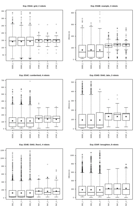
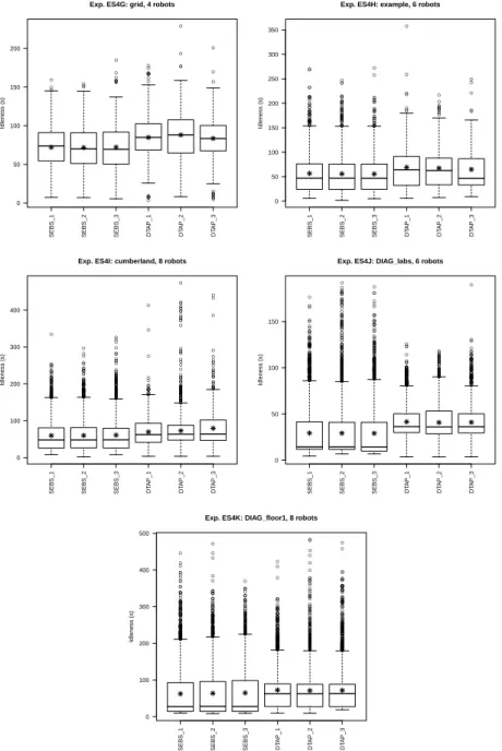
5. Initial poses of the robots. For the initial poses of the robots we have consid-ered two situations: 1) robots start in predefined positions (the same in all the experiments for a given map and a given number of robots and the same used in previous experiments by other authors) that are scattered through the environ-ment; 2) robots start from a cluster of positions close each other; this set-up is a

more realistic one in which we assume robots are all started from a given starting area. As shown in a set of specific experiments, when most effective algorithms are considered (SEBS and DTAP in our case), the initial position of the robot does not affect significantly the overall performance.

In summary, the main factor that increases variability of the experimental results is the obstacle avoidance behavior, that is activated to solve interferences. As already mentioned, we have added the interferences as a performance metric. Moreover, we have implemented a mechanism to detect when results are strongly affected by the obstacle avoidance procedure. More specifically, we have stopped all the experiments in which a robot is not able to reach a target location within 5 minutes. These experi-ments are not considered in the results, since the performance based on the idleness is not suitable for a fair comparison with another run in which this situation did not oc-cur. Moreover, as explained in the next section, we have discarded all the experiments that have low correlation with the majority.

5.3 Performance metrics

In order to assess the performance of a MRP system, several performance metrics and evaluation procedures have been proposed in previous work. Most of them are based on the concept of idleness that measures time distance between two consecutive visits of a node by any robot in the team. Therefore, as already mentioned,global idleness average IG

avg,global idleness standard deviation IstddevG , andglobal maximum idleness I_maxG are typical performance metrics used to compare different systems. However, it is important to notice that very often a trade-off among these metrics allows for a better comparison of different algorithms.

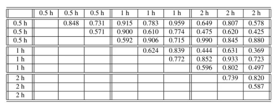
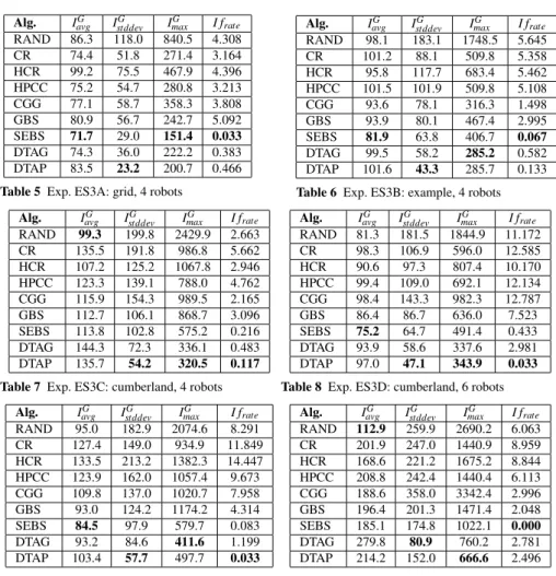
In this section, we discuss the results of a first set of experiments (named Ex-periment Set 1) aiming at presenting and discussing the different performance met-rics and their visualization. The experiments have been performed in the following settings: Cumberland map with 4 robots, 1 hour of duration, and three algorithms compared: a random method (RAND) in which each robot selects the next target node randomly among the adjacent ones, SEBS algorithm [22], and DTAP algorithm described in this article. For each algorithm, three runs have been executed. In the following, we present the results of this experiment in different forms in order to discuss them in details.

A first representation of the results is given in Table 3, which reports the values I_avgG ,I_stddevG , andI_maxG for each run. This is the typical way in which MRP results have been presented in previous papers.

From this table, it is possible to notice that the difference among the average val-uesIG

avg in the different runs in some cases is not statistically significant, given the high standard deviation. Moreover, the RAND algorithm has even generally better performance if only the average idleness is considered, but this is obtained at the cost of a substantially higher standard deviation and maximum value. Both SEBS and DTAP have significant lower standard deviation and maximum values. The dif-ferences between SEBS and DTAP are further analyzed in the next sections. This

Algorithm IG

avg IstddevG ImaxG I frate

RAND 1 117.2 216.2 2066.0 6.857 RAND 2 99.3 199.8 2429.9 2.663 RAND 3 102.6 201.6 2044.8 2.848 SEBS 1 114.3 100.3 567.1 0.100 SEBS 2 113.8 102.8 575.2 0.216 SEBS 3 112.8 102.4 687.4 0.283 DTAP 1 142.6 57.1 371.3 0.167 DTAP 2 140.2 55.4 306.9 0.083 DTAP 3 135.7 54.2 320.5 0.117

Table 3 Exp. ES1: cumberland, 4 robots, RAND, SEBS, and DTAP algorithms. Best values in bold.

table shows also the number of interferences per minute (last column) that is a metric explained later in this section.

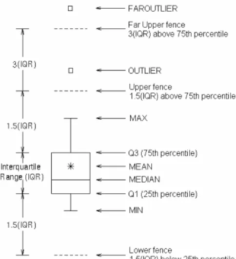
Fig. 2 Meaninf of boxplot representation.

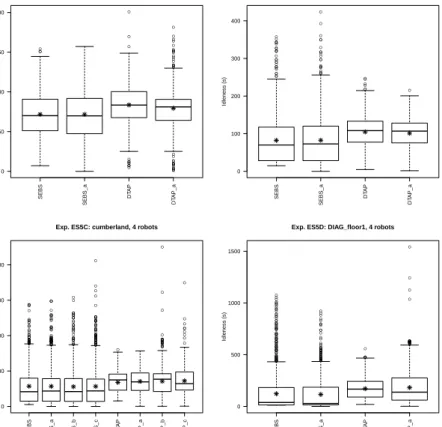
A different format for representing the results of a MRP task is given byboxplots, whose definition is presented in Figure 2. Figure 3 shows the same results of this experiment using boxplots. From this view, the difference between the algorithms appears more clearly. RAND algorithm achieves a low average thanks to many small values and a few high ones, while SEBS and DTAP provide for a more balanced set of values having smaller standard deviation and few outliers and high values.

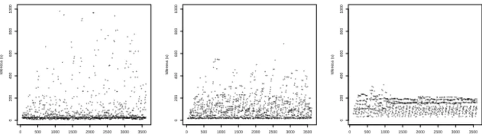
Another view of the results is given in the form of a temporal plot of idleness values over the time of an experimental run. Figure 4 shows a plot for one run for each of the algorithms considered in this experiment. From these plots, we can analyze the distribution of the idleness values and the temporal evolution of the performance metrics. We can see that the majority of values in RAND are low values, while in

● ● ● ● ● ● ● ● ● ● ● ● ● ● ● ● ● ● ● ● ● ● ● ● ● ● ● ● ● ● ● ● ● ● ● ● ● ● ● ● ● ● ● ● ● ● ● ● ● ● ● ● ● ● ● ● ● ● ● ● ● ● ● ● ● ● ● ● ● ● ● ● ● ● ● ● ● ● ● ● ● ● ● ● ● ● ● ● ● ● ● ● ● ● ● ● ● ● ● ● ● ● ● ● ● ● ● ● ● ● ● ● ● ● ● ● ● ● ● ● ● ● ● ● ● ● ● ● ● ● ● ● ● ● ● ● ● ● ● ● ● ● ● ● ● ● ● ● ● ● ● ● ● ● ● ● ● ● ● ● ● ● ● ● ● ● ● ● ● ● ● ● ● ● ● ● ● ● ● ● ● ● ● ● ● ● ● ● ● ● ● ● ● ● ● ● ● ● ● ● ● ● ● ● ● ● ● ● ● ● ● ● ● ● ● ● ● ● ● ● ● ● ● ● ● ● ● ● ● ● ● ● ● ● ● ● ● ● ● ● ● ● ● ● ● ● ● ● ● ● ● ● ● ● ● ● ● ● ● ● ● ● ● ● ● ● ● ● ● ● ● ● ● ● ● ● ● ● ● ● ● ● ● ● ● ● ● ● ● ● ● ● ● ● ● ● ● ● ● ● ● ● ● ● ● ● ● ● ● ● ● ● ● ● ● ● ● ● ● ● ● ● ● ● ● ● ● ● ● ● ● ● ● ● ● ● ● ● ● ● ● ● ● ● ● ● ● ● ● ● ● ● ● ● ● ● ● ● ● ● ● ● ● ● ● ● ● ● ● ● ● ● ● ● ● ● ● ● ● ● ● ● ● ● ● ● ● ● ● ● ● ● ● ● ● ● ● ● ● ● ● ● ● ● ● ● ● ● ● ● ● ● ● ● ● ● ● ● ● ● ● ● ● ● ● ● ● ● ● ● ● ● ● ● ● ● ● ● ● ● ● ● ● ● ● ● ● ● ● ● ● ● ● ● ● ● ● ● ● ● ● ● ● ● ● ● ● ● ● ● ● ● ● ● ● ● ● ● ● ● ● ● ● ● ● ● ● ● ● ● ● ● ● ● ● ● ● ● ● ● ● ● ● ● ● ● ● ● ● ● ● ● ● ● ● ● ● ● ● ● ● ● ● ● ● ● ● ● ● ● ● ● ● ● ● ● ● ● ● ● ● ● ● ● ● ● ● ● ● ● ● ● ● ● ● ● ● ● ● ● ● ● ● ● ● ● ● ● ● ● ●

RAND_1 RAND_2 RAND_3 SEBS_1 SEBS_2 SEBS_3 DT

AP_1 DT AP_2 DT AP_3 0 500 1000 1500 2000 2500

Exp. ES1: cumberland, 4 robots

Idleness (s)

Fig. 3 Boxplots of comparison among the three algorithms.

● ● ● ●● ● ● ●● ● ●●●●●● ● ● ● ●●●● ● ●●● ● ●● ● ● ● ● ● ● ●● ● ●● ● ● ● ● ● ● ●●● ● ●● ● ●●●●● ● ● ● ● ● ●●● ● ● ●● ●● ● ●● ● ● ●●●●● ● ● ● ● ● ● ● ● ● ● ●● ● ●●● ●●● ● ● ● ● ●● ● ● ● ●● ● ● ● ● ●●●●● ● ● ● ● ●●● ● ● ● ● ● ● ● ● ● ● ● ● ● ● ● ●●● ● ● ● ●●●●●● ● ●● ● ●●●●●●● ● ● ● ●●● ● ● ● ●● ● ● ● ● ● ● ● ● ● ● ●●● ● ● ● ● ● ● ● ● ●● ● ●● ● ● ● ● ●●● ● ● ● ● ● ● ●● ● ●● ● ● ● ● ●● ●● ● ●● ● ● ● ● ● ● ●● ● ● ● ●● ●● ● ● ● ●● ● ● ● ●● ● ● ● ● ● ● ● ● ● ●●●● ● ●●●●●● ● ● ● ●● ●● ● ● ● ● ●● ● ● ● ●● ● ● ● ●●●● ●● ● ● ● ● ● ●● ● ●● ● ● ● ● ● ● ● ● ● ● ●●● ● ● ●● ● ●● ● ●● ● ●● ●●● ● ● ●● ● ● ● ●● ●●●●● ● ●● ● ● ● ●● ● ● ● ●● ● ● ●●● ● ●●● ● ● ● ● ●●● ● ●● ● ● ●●● ● ● ● ●●●● ● ● ● ●●●● ● ● ● ● ● ●● ● ● ● ● ● ● ● ● ● ● ●● ● ● ● ● ● ●●● ● ●● ● ● ● ● ● ● ● ●● ● ● ● ● ● ●● ● ●●●●● ● ● ●●●● ●● ● ● ● ●●● ● ● ● ● ●●●● ● ● ● ●● ● ● ●● ● ●●●● ● ● ●● ● ● ● ●●● ● ● ● ● ● ● ● ● ● ● ● ●●● ● ● ● ● ●●● ● ● ● ● ●● ● ● ● ● ●●●●● ● ● ● ● ● ● ● ●●●● ● ● ● ●●● ● ●● ● ● ● ●●● ● ● ● ● ● ● ● ● ●●●● ●● ● ● ● ● ● ● ●●● ● ● ● ●● ● ●●● ● ● ● ● ● ●●●● ● ●●●●● ● ● ●●● ● ● ● ● ● ●●●● ● ●●●●●●● ● ● ●● ● ●● ● ● ● ●● ● ● ● ● ●● ● ●● ●● ●● ●●● ● ●● ● ● ●● ● ●●●● ● ● ●●● ● ● ●● ● ● ● ● ● ● ● ● ● ● ●●● ● ● ● ● ● ●● ● ● ● ● ● ●●● ● ●● ● ●● ●● ● ● ● ● ● ●●●●● ● ● ●●● ● ● ● ● ● ● ●● ● ● ● ● ● ●● ● ● ●● ●● ● ●●● ● ●● ● ●● ● ● ● ● ●● ● ● ●●●● ● ● ● ● ●●●● ● ● ● ● ● ● ●●● ● ● ● ● ● ●●● ● ● ● ● ●●● ●● ● ● ● ● ● ● ● ● ● ● ● ● ● ●●●● ● ● ● ● ●● ● ●●●●● ● ● ● ● ● ● ●● ● ● ● ● ●●● ● ● ● ● ● ● ● ● ● ●● ●●● ●● ● ● ●●● ● ● ● ●●● ● ●● ● ● ● ●● ● ●● ●● ●● ● ● ● ● ●● ● ● ●●●●●●●●●● ● ● ●●● ● ●● ● ● ●● ● ● ● ●●●●● ● ● ● ● ●● ● ● ● ● ● ● ● ●●●●●● ● ● ● ● ●● ●● ● ● ● ● ● ● ● ● ● ● ● ● ● ●●●● ● ● ● ● ● ● ● ● ● ● ●●●● ● ● ● ● ●●●● ● ● ●● ● ● ● ● ● ● ●● ● ● ●● ● ●●● ● ● ● ●● ● ●● ● ● ●●● ● ● ● ● ●● ● ● ● ● ● ●● ● ● ● ● ●●●●● ● ● ● ● ● ●● ● ●●●●●●●● ● ● ●●●● ● ●● ● ●● ● ● ● ● ●● ● ● 0 500 1000 1500 2000 2500 3000 3500 0 200 400 600 800 1000

Exp. ES1: cumberland, 4 robots RAND_3

Time (s) Idleness (s) ●●●●● ● ●● ● ●● ● ● ● ● ●● ●● ● ● ● ●●●● ●●● ● ●● ● ● ● ●● ● ● ● ● ● ● ●● ● ● ● ● ● ● ● ● ● ● ● ● ● ● ● ● ● ● ● ● ●● ● ● ● ● ● ● ● ● ● ● ● ● ● ● ● ●●● ● ● ● ● ● ● ●●●● ● ● ● ● ● ● ● ● ● ● ● ● ● ● ● ● ● ● ● ● ● ● ●● ● ● ● ● ● ● ●● ● ● ● ● ●●● ● ● ● ● ● ● ● ● ● ● ● ●● ● ● ● ● ● ● ●● ● ● ● ● ● ● ● ●● ● ● ● ● ● ● ●● ● ● ● ●● ●● ● ● ● ● ● ● ● ● ● ● ● ● ● ● ● ● ● ● ● ● ● ● ●● ● ● ● ● ● ● ● ● ● ● ● ● ● ● ●● ● ● ● ●● ● ● ● ● ● ● ● ● ●● ● ● ●●● ● ● ● ● ● ● ● ● ● ● ● ● ● ● ● ● ● ● ● ● ● ● ● ● ● ● ● ● ● ● ● ● ● ● ● ● ● ● ●● ● ● ●● ● ● ● ● ● ● ● ● ● ● ● ● ● ● ● ● ● ● ● ●● ● ● ● ● ● ●● ● ● ● ●● ● ● ● ●● ● ● ● ● ● ● ● ● ●● ● ● ● ● ● ● ● ● ●● ● ●●● ● ● ● ● ● ● ● ● ● ●● ● ● ●● ●●●● ● ● ● ● ● ● ● ● ● ● ● ● ● ● ● ● ● ● ● ● ● ● ● ● ●● ● ● ● ●●● ● ●● ● ● ● ● ● ● ● ● ● ● ● ● ● ● ● ● ● ● ● ● ● ● ● ● ● ● ● ● ● ● ● ● ● ● ● ● ● ●● ● ● ● ● ● ● ● ● ● ● ● ● ● ● ●● ● ● ● ●● ● ● ●●● ● ● ● ● ● ● ● ● ● ● ● ● ●● ● ● ● ● ● ● ● ● ● ● ● ● ● ● ● ● ● ● ● ● ● ●● ● ● ●● ● ● ● ● ● ● ● ● ● ● ● ●● ● ● ● ● ● ●● ● ● ● ● ● ● ● ● ● ● ● ● ● ● ●● ● ● ●● ● ● ● ● ● ●● ●● ● ● ● ● ● ● ●● ● ● ● ● ● ● ● ● ●● ● ● ● ●● ● ●● ●● ● ● ● ● ●● ● ●● ●● ● ● ● ● ● ● ● ● ● ● ● ● ● ● ● ● ● ● ● ●● ● ● ● ● ● ● ● ● ● ● ●●● ● ● ● ● ● ● ● ● ●● ● ● ● ● ● ● ● ● ● ● ● ● ● ● ● ● ● ● ● ● ● ● ● ● ● ● ● ● ● ● ● ● ● ●●●● ● ● ● ● ● ● ●● ● ● ●● ● ● ● ●● ● ● ● ● ●● ●●● ● ● ● ● ● ● ● ● ● ● ●● ● ● ● ● ● ● ● ● ● ● ● ● ● ● ● ● ● ● ● ● ● ● ● ● ● ● ● ● ● ● ● ● ● ● ● ● ● ● ● ● ● ● ●● ●●● ●● ● ● ● ●● ●● ●● ● ● ● ● ● ● ● ● ● ● ● ●● ● ● ● ●● ● ●● ● ● ● ● ● ● ● ● ● ● ● ● ● ● ● ● ● ● ● ● ● ● ●● ● ● ●● ● ● ●● ● ● ● ● ● ● ● ● ● ● ● ● ● ● ●● ● ● ● ● ● ● ● ● ● ● ● ● ● ● ● ● ● ● ● ●● ● ● ● ● ● ● ● ● ● ● ● ● ● ● ● ●● ● ● ● ● ● ● ● ●● ● ● ● ● ● ● ● ● ● ●● ● ● ● ● ● ●● ● ● ● ● ● ● ● ● ● ● ● ● ● ● ● ● ● ● ● ● ● ● ● ● ● ● ● ●●● ● ● ● ● ● ● ● ● ● ● ● ● ● ● ● ● ● ● ● ● ● ● ●● ● ● ● ● ● ● ● ● ● ● ● ● ● ●● ● ● ● ● ● ● ● ● ● ● ●● ● ●● ● ● ● ● ● ● ● ● ● ●● ● ●● ● ● ● ● ● ● ● ● ● ● ● ● ● ● ● ● ● ● ● ●● ● ● ● ● ●● ● ●● ● ●● ● ● ● ● ● ● ● ● ● ● ● ● ● ● ● ● ● ● ● ● ● ● ● ● ● ● ● ● ● ● ●● ● ● ● ● ●● ● ● ● ● ●● ● ● ● ● ●● ● ● ● ● ● ● ● ● ● ● ● ● ● ● ● ● ● ● ● ● ●● ● ● ● ● ● ● ● ● ●●● ● ● ● ● ● ● ● ● ●● ● ● ●● ● ● ● ● ● ● ● ● ● ● ● ● ● ● ● ● ● ● ● ● ● ● ● ● ● ● ● ● ● ●● ●●●● ● ● ● ● ● ● ●● ● ● ●● ● ● ● ●●●● ● ●● ●● ● ● ● 0 500 1000 1500 2000 2500 3000 3500 0 200 400 600 800 1000

Exp. ES1: cumberland, 4 robots SEBS_3

Time (s) Idleness (s) ●● ● ● ● ● ● ● ●● ● ● ● ● ● ● ● ● ● ● ● ● ● ● ● ● ● ● ● ● ● ● ● ● ● ● ● ● ● ● ● ● ● ●● ● ● ● ● ● ● ● ● ●● ● ●● ● ● ● ● ● ● ● ● ● ● ● ● ● ● ● ● ● ● ● ● ● ● ● ● ● ● ● ● ● ● ● ● ● ● ● ● ● ● ● ● ● ● ● ● ● ●● ● ● ● ● ●● ● ● ● ● ●● ● ● ● ● ●● ● ● ● ● ● ● ● ● ● ● ● ● ●● ● ● ● ● ● ● ● ● ● ●● ● ● ● ● ● ● ● ● ● ● ● ● ● ● ● ● ● ● ● ● ● ● ● ● ● ● ● ● ● ● ● ● ● ● ● ●● ● ● ● ● ● ● ● ● ●● ● ●● ● ● ● ● ● ● ● ● ● ● ● ● ● ● ● ● ● ● ● ● ●● ● ● ● ● ● ● ● ●● ● ● ● ● ● ●● ●● ● ● ● ● ● ● ● ●● ● ● ● ● ● ● ● ● ● ●● ● ● ● ● ● ● ● ● ● ● ● ● ● ● ● ● ● ● ● ● ● ● ● ● ● ● ● ● ● ●● ● ●●● ● ● ● ● ● ● ● ● ● ● ● ● ● ● ● ● ● ● ● ● ● ● ● ● ● ●● ●● ● ● ●● ● ● ● ● ●● ● ● ● ● ● ● ● ● ● ● ● ●● ● ● ● ● ● ● ● ● ● ● ● ● ● ● ● ● ● ●● ● ● ● ● ● ● ● ● ● ●● ● ● ● ● ● ●● ●● ● ● ● ● ● ● ● ● ● ● ● ● ● ● ● ● ● ● ●● ● ●●●● ● ●● ● ● ●● ●● ● ●● ● ● ● ●● ● ● ●● ● ●● ● ● ●●● ● ● ● ● ●● ●● ● ●● ● ● ● ●● ● ● ●●● ● ●● ● ●●● ●● ●● ● ● ●● ● ● ● ● ● ● ●● ● ● ● ● ●●● ●● ● ● ●● ● ● ● ● ● ●● ● ● ● ● ● ● ● ● ● ●● ● ● ● ● ● ● ● ● ● ● ● ● ●● ● ● ● ● ● ● ● ● ● ● ● ● ● ●● ● ● ●● ● ● ● ●●● ● ● ● ●● ● ● ● ● ● ● ● ●● ● ● ● ● ●● ● ● ● ● ● ● ● ● ● ● ● ● ● ● ● ● ● ●● ● ● ● ● ● ●● ● ● ● ● ● ● ● ● ● ● ● ● ● ● ● ●● ● ● ●● ● ●● ● ● ● ●●● ● ●● ● ● ● ● ● ● ● ● ● ● ●● ● ● ● ● ● ●● ●● ● ● ● ● ● ● ● ● ● ● ● ● ● ●● ● ●● ● ● ● ● ● ● ● ● ● ● ● ● ● ● ●● ● ●● ● ●● ● ● ●●● ● ● ● ● ● ● ● ● ● ● ● ● ● ● ● ● ● ● ● ● ● ● ● ● ● ● ● ● ● ● ● ● ● ● ●● ● ●● ● ●● ● ● ● ● ● ● ● ● ● ●●● ● ● ●● ● ● ● ● ● ● ● ●● ● ●● ● ● ● ● ●●● ● ● ● ● ● ● ● ● ● ● ● ● ● ●●● ● ● ●● ● ● ● ● ●● ● ● ● ● ● ● ● ● ● ● ● ● ● ● ● ● ● ● ● ● ● ●●● ● ● ● ● ● ●● ● ● ● ● ●● ● ● ● ● ● ●● ● ●● ● ●● ● ● ●● ●●● ● ● ● ●● ●● ●● ● ● ●● ● ● ● ●●● ● ● ● ●● ● ● ● ●● ●● ● ● ● ● ● ● ● ● ● ● ●● ● ● ● ● ● ● ● ● ● ● ● ● ●●● ● ● ●● ● ● ● ● ● ● ● ● ●● ● ●●●●● ● ● ● ● ●● ● ●● ● ● ● ● ● ● ● ● ● ● ● ● ● ● ● ● ●● ● ●●● ● ● ● ● ● ● ●● ● ● ● ● ● ● ● ● ● ● ● ● ● ● ● ● ●● ●● ●● ● ● ● ● ● ● ●● ● ● ● ●●● ● ●● ● ● 0 500 1000 1500 2000 2500 3000 3500 0 200 400 600 800 1000

Exp. ES1: cumberland, 4 robots DTAP_3

Time (s)

Idleness (s)

Fig. 4 Temporal plots of comparison among the three algorithms: RAND, SEBS, DTAP.

DTAP the majority of values are around 200 seconds. Notice also that some values in RAND are not shown in the leftmost figure, since the idleness scale (Y axis) has been limited to 1000 s, while RAND generates values also above this limit. Finally, temporal plots are useful to see if an algorithm has some transient behavior. For example, in DTAP 3 outliers are present only in the first phase of the experiment. A

more detailed analysis of temporal evolution of performance is presented in Section 5.8.

In addition to these metrics based on the idleness, we also measure the number of interferencesover time. An interference is defined as a situation when two robots get closer so that the obstacle avoidance module is used to avoid each other. In the simu-lated experiments, the interferences are detected when two robots are within 2 meters and they are counted by an external module accessing the ground truth positions of the robots. The interferences are important, since they affect the time to reach a goal position and thus all the performance metrics based on idleness. Moreover, they can-not just be disregarded, since minimizing conflicts on space is an important feature of a multi-robot patrolling system. In the experiments reported in this article, we use the rate of interferences (I frate), expressed in number of interferences per minute, as an additional performance metric of an MRP system. The results forI frate obtained in the experiments reported in this section are illustrated in the last column of Table 3. As expected, SEBS and DTAP algorithms present much less interferences with respect to the RAND algorithm.

From this analysis, we can conclude that using only the average valueI_avgG would not allow for a suitable comparison of different methods. The use of boxplots and temporal plots provides for a detailed analysis of the performance of the algorithm. However, in these cases, it is difficult to summarize the result of an experiment in a single value and thus it is not always possible to definitely compare two sets of results. The use of the maximum valueI_maxG is a good choice as worst case analysis, but from the experiments done during this work we have experienced a high variability of this value (since it depends on noise and uncertainty in the execution of the task by the robots, which is not modeled in the MRP problem). Finally, the rate of interferences I frateis important to assess the ability of the algorithm to prevent space conflicts.

In the following, we mainly present the results of experiments with boxplots of idleness values. In some cases, we also show temporal plots, in order to evaluate temporal evolution of the idleness, and tables with the aggregate results based on the idleness and the rate of interferences.

5.4 Length and repetitions of the experiments

Given the external factors mentioned in the previous section, it is important to de-termine how many experiments in the same setting are needed in order to guarantee significant results and how long an experiment must last. To this end, we made the experiments reported below (namedExperiment Set 2).

Because of the above mentioned external factors that affect the results of a MRP test, performing a single run of an experiment in a given setting is not enough to guar-antee significant results. The procedure we have developed in this article is based on performing a statistical test (in particular, the one-way ANOVA test) to the obtained results in order to determine the ones that are significant. More specifically, we per-form many runs of each configuration until we are able to collect at least 3 tests that have significant correlation. Significant correlation is measured with the ANOVA test applied to all the values of the idlenesses collected during an experiment. When the