CIVIL ENGINEERING
Prediction of scour caused by 2D horizontal jets
using soft computing techniques
Masoud Karbasi
a,*, H. Md. Azamathulla
ba
Hydraulic Structures, Water Engineering Dep., Faculty of Agriculture, University of Zanjan, Zanjan, Iran
bCivil Engineering, Faculty of Engineering, University of Tabuk, Tabuk, Saudi Arabia
Received 6 December 2015; revised 1 March 2016; accepted 9 April 2016
KEYWORDS
2D horizontal jets; Scour hole; Sluice gate; Soft-computing
Abstract This paper presents application of five soft-computing techniques, artificial neural net-works, support vector regression, gene expression programming, grouping method of data handling (GMDH) neural network and adaptive-network-based fuzzy inference system, to predict maximum scour hole depth downstream of a sluice gate. The input parameters affecting the scour depth are the sediment size and its gradation, apron length, sluice gate opening, jet Froude number and the tail water depth. Six non-dimensional parameters were achieved to define a functional relationship between the input and output variables. Published data were used from the experimental researches. The results of soft-computing techniques were compared with empirical and regression based equa-tions. The results obtained from the soft-computing techniques are superior to those of empirical and regression based equations. Comparison of soft-computing techniques showed that accuracy of the ANN model is higher than other models (RMSE= 0.869). A new GEP based equation was proposed.
Ó2016 Faculty of Engineering, Ain Shams University. Production and hosting by Elsevier B.V. This is an open access article under the CC BY-NC-ND license (http://creativecommons.org/licenses/by-nc-nd/4.0/).
1. Introduction
Scour is a regular phenomenon of bringing down the riverbed level because of the evacuation of sediment by the erosive activity of a flowing stream. Local scour is produced close to the structures because of adjustment of the stream field as an
obstacle to the stream by the structures. Turbulent horizontal jets appear when flow is discharged through underflow gates and rectangular culverts[1].
The scour phenomenon downstream of a sluice gate is com-plex in nature due to rapid change of the flow characteristics on the sediment bed[2]. Local scour downstream of hydraulic structures by a jet issuing from a sluice gate has gotten impres-sive consideration in light of the fact that scour can jeopardize the foundation of the structure.
Laboratory study of scour downstream of sluice gates has been conducted by several researchers[2–16].
Dey and Sarkar [2] performed an experimental study on
scour hole characteristics over a wide range of sediment size, tailwater depth, sluice opening and apron length and con-cluded the following results: The equilibrium scour depth,
* Corresponding author. Tel.: +98 2433052388, +98 9123416540. E-mail addresses:[email protected](M. Karbasi), [email protected](H. Md. Azamathulla).
Peer review under responsibility of Ain Shams University.
Production and hosting by Elsevier
Ain Shams University
Ain Shams Engineering Journal
www.elsevier.com/locate/asej www.sciencedirect.com
decreases with increase in sediment size and sluice opening. The equilibrium scour depth increases with rise in densimetric Froude number, and for a higher densimetric Froude number, the equilibrium scour depth is free of the densimetric Froude number. No uniformity of sediments decreases the scour depth downstream of the launching apron. Placing a launching apron decreases the scour depth.
Hamidifar et al. [9] examined the scour behaviors of the
non-cohesive sediments downstream of smooth and rough aprons. The results showed that the principle attributes of the scour holes, such as the maximum scour depth and its dis-tance from the end of the apron, the maximum extension of the hole, the dune height and its distance from the end of the apron, were much lower for rough than smooth aprons.
In spite of the reported experimental data sets, it is hard to thoroughly catch the impacts of the different parameters on the scour created in view of restrictions in the laboratory facil-ities and scope of tests that can be led. Thus, traditional methodologies utilizing regression-based techniques to predict the scour depth are regular. The empirical equations proposed by these procedures are fundamentally confined to the range of the database utilized in their derivation[17].
Recently, different artificial intelligence techniques such as
artificial neural network (ANN) [18–29], adaptive
neuron-fuzzy inference system (ANFIS) [20,30–38], support vector
machine (SVM) [29,36,39–41], decision trees [22,41–44],
genetic programming (GP) [45–47], linear genetic
program-ming (LGP) [48,49], gene expression programming (GEP)
[27,28,50], group method of data handling (GMDH), data mining[17,51–59], and machine learning method were utilized for modeling of problems in scour prediction.
Najafzadeh and Lim[17]developed structure of a
neuro-fuzzy GMDH network as a self-organized method to estimate the scour depth downstream of a sluice gate with an apron. An evolutionary algorithm of PSO is developed with the NF-GMDH network for the training stage. The results indicated that the NF-GMDH–PSO network produced lower error in scour prediction than all other models.
This paper presents the modeling of local scour depth downstream of a sluice gate utilizing soft computing tech-niques: ANNs, SVR, GMDH, ANFIS and GEP. Results of soft computing techniques were compared with empirical and multiple regression based equations and finally a new GEP based equation was proposed.
2. Methods
2.1. Theoretical background
A definition sketch for local scour due to 2D horizontal jets is indicated inFig. 1, which represents a typical condition of a local scour hole downstream from a sluice gate.
Local scour due to horizontal jets is influenced by the power of the jet, the size and uniformity of the bed material, the presence of an apron between the jet inlet and the erodible bed, and the tailwater depth. Most existing scour equations use gate opening as the major length scale for equilibrium local
scour depth [1]. Maximum equilibrium scour depth
down-stream of a sluice gate, can be given in functional form as[2]:
Ds¼u U;q;qs;g;m;b;La;ht;d50;rg
ð1Þ where U= issuing velocity of jet;m= kinematic viscosity of
water; q= density of water; qs= density of sediments;
b= gate opening; g = gravitational acceleration;La= apron
length; ht= tailwater depth; d50= median sediment size,
rg= sediment gradation.
Applying the Buckinghamptheorem, one gets
Ds b ¼w U ffiffiffiffiffi gb p ;Umb;qsq;La b ; d50 b ; ht b;rg ð2Þ The kinematic viscosity may not affect the scour depth in turbulent flow[60]and the ratio ofqs
q is constant and can be
neglected. As a result the final equation is derived as follows:
Ds b ¼w U ffiffiffiffiffi gb p ;La b ; d50 b ; ht b;rg ð3Þ Notation b gate opening
d50 median sediment size
ei prediction error
e mean prediction error
Frj jet Froud number
g acceleration due to gravity
ht tailwater depth
La apron length
n number of data
Oi observed value
Qi mean value of observations
Pi predicted value
Pi mean value of predictions
R jet hydraulic radius
Se standard deviation of the prediction errors
U velocity of jet
w sediment fall velocity
q mass density of water
qs mass density of sediments
lAiðxÞ fuzzy membership function
m kinematic viscosity of water
rg sediment gradation
Figure 1 Definition sketch for local scour due to 2D horizontal jets.
2.2. Available experimental data
A large number of experimental data for 2D horizontal jets
have been published. The 273 laboratory data inTable 1are
utilized in the analysis presented in this paper. Statistical
parameters of the train and test data are shown in Table 2.
The training data were used for learning process and test data were used to evaluate the performance of the different models.
2.3. Experimental based empirical equations
Melville and Lim [1] analyzed 309 laboratory data for local
scour depth and developed a new prediction equation.
Ds
b ¼3FrjKDKhtKrKL ð4Þ
whereFrjis jet Froude number U=
ffiffiffiffiffi gb p ;KDis sediment size effect: KD¼1 for d50 b <0:6 andKD¼0:6 d50 b 1 for d50 b P0:6 KLis apron length effect:
KL¼1tanh
0:013La b
Kytis tailwater depth effect:
Kht¼1 for ht b >6 andKD¼0:01 ht b 2:6 for ht b66 Kris sediment gradation effect:
Kr¼1 forrg62:2 andKr¼1:2rg0:34 forrg>2:2
Selection of prediction equations for scour caused by 2D horizontal jets has been presented inTable 3.
2.4. Regression analysis
One of the traditional issues in statistical analysis is to discover a suitable relationship between a feedback variable and a set of input variables. Regression analysis is normally used to por-tray quantitative connections between a feedback variable and one or more informative variables. In MLR, the function is a linear mathematical statement, i.e. straight-line, in the form:
Y¼a0þa1X1þa2X2þ þanXn ð5Þ
where Y is the response variable, a0–an are the equation
parameters for the linear equation, and,X1–Xn are the
inde-pendent variables[61].
Multiple nonlinear regression (MNLR) is a manifestation of regression analysis in which observational information is modeled by a function, which is a nonlinear combination of the model parameters and relies on one or more independent
Table 1 Laboratory data for scour depth caused by 2D horizontal jets issuing from sluice gates.
Researcher Number of data Ds=b Frj ht=b d50=b La=b rg Dey and Sarkar[2] 213 1.5–8.2 2.4–4.9 9.1–12.8 0.02–0.50 27–55 1.1–3.9 Aderibigbe and Rajaratnam[4] 32 1.3–32.7 1.2–21.5 6.9–60.0 0.05–1.35 0 1.3–3.1 Chatterjee et al.[7] 28 0.9–4.1 1.0–5.5 5.8–15.5 0.02–0.14 13–33 1.2–1.4
Table 2 Descriptive statics of train and test data.
Variable Data range Mean Standard deviation
Train Test Train Test Train Test
Ds=b 0.6–24.4 0.5–21.7 12.5 11.10 3.20 3.87 Frj 1.23–21.54 1.02–17.43 11.38 9.22 2.36 2.71 ht=b 3.66–65.73 5.7–65.73 34.7 35.72 11.17 13.54 d50=b 0.017–1.35 0.015–1.35 0.684 0.683 0.198 0.204 La=b 0–60 0–60 30 30 12.75 14.00 rg 1–3.89 1–3.92 2.445 2.460 0.645 0.678
Table 3 Selection of prediction equations for scour depth downstream of sluice gate. Researcher Equation
Dey and Sarkar[2] Ds
b ¼2:59ðFrdjÞ 0:94 ht b 0:16 La b 0:37 d 50 b 0:25 Frdj¼½ðS Uj G1Þgd500:5 Lim and Yu[11] Ds b ¼1:04ðFrdjÞ 1:47 d50 b 0:33 r0:69 g KLKL¼exp0:004ðFrdjÞ0:35rg0:5 db50 0:5 ðLa bÞ 1:4 h i Chatterjee et al.[7] Ds b ¼0:775Frj Ali and Lim[5] Ds
R¼2:3ðFrdjÞ 0:75 Uj w 0:5 d50 R 0:375
1:19 whereR= jet hydraulic radius; andw= sediment fall velocity Altinbilek and Basmaci[6] Ds
b ¼ db50tan/ 0:5
variables[62]. Dissimilar to customary MLR, which is limited to estimating linear models, MNLR can estimate models with nonlinear relationships between input and response variables. The general presentation of the nonlinear relation is assumed to be the following: Y¼b0X b1 1 X b2 2 . . .X bn n ð6Þ
whereb0–bnare the equation parameters. 2.5. Artificial neural network
Artificial neural networks as the most well-known artificial intelligence models are an accumulation of neurons with par-ticular structure formed based on the relationship between neurons in different layers[63]. Neuron is a mathematical unit, and an artificial neural network that comprises of neurons is a complex and nonlinear framework. A static ANN known as a multilayer perceptron (MLP) is the most applied ANN in dis-tinctive fields of engineering. Application of the artificial neu-ral networks in the field of water resources and hydraulic
engineering has grown quickly in the recent decade [63]. An
ANN typically comprises of three layers: the input layer, where the data are introduced to the network; the hidden layer or lay-ers, where data are processed; and the output layer, where the results of given input are produced[64]. A multi-layer feed-forward back-propagation neural network with one hidden (median) layer has been used in the present study[65]. In a feed-forward back-propagation neural network, the weighted connections feed activations only in the forward direction from an input layer to the output layer. These interconnections are adjusted utilizing an error convergence technique so that the network’s response best matches the desired response. The major superiority of the ANN technique over conventional methods is that it does not require information about the com-plex nature of the process[64].
In this study one hidden layer including 5 neurons was used for the neural networks model. Too few neurons give a poor fit on unseen data, while too many neurons result in over-training of the net on the training set. Back-propagation algorithm was used as a training algorithm in this study.
2.6. Support vector regression
Classification of data is a routine task in data-driven modeling. Utilizing support vector machines, we can apart classes of data by a hyper plane. A support vector machine (SVM) is a con-cept for a set of related supervised learning methods that ana-lyze data and recognize patterns, used for classification and
regression analysis [63]. Support vector machine was
devel-oped by Vapnik in 1995 [66]. The basic difference between
the application of SVM for regression (SVR) and the applica-tion of SVM for classificaapplica-tion is that in SVR output is
consid-ered as a real number instead of a binary number[63]. The
detail computation procedure can be found in[66].
2.7. Adaptive Neuro-Fuzzy Inference System
Adaptive Neuro-Fuzzy Inference Systems were developed by Jung in 1993. Neuro-fuzzy model combines artificial neural network (ANN) and fuzzy inference system (FIS) to facilitate the process of learning and adaption. In neuro-fuzzy models, a
multilayer feed forward neural network is used to identify the parameters of an adaptive network fuzzy inference system. Importantly, fuzzy logic allows the communication between the input space and output space with a list of If-then sen-tences, called law. Having a method that uses the data to con-struct these rules is considered as an efficient tool. On the other hand, capabilities of artificial neural networks for training, using different educational models can establish the relation-ship between input and output variables. Therefore, the com-bination of fuzzy inference system and artificial neural network as a powerful tool that can predict the results of numerical data is available, as adaptive neuro-fuzzy inference system is introduced. This system of neural networks and fuzzy logic algorithms is used to design nonlinear mapping between input and output spaces.
ANFIS consists of five layers (Fig. 2):
Layer 1:input nodes. Each node of this layer creates mem-bership grades based on the proper fuzzy set they belong to using membership functions. The node output O1,iis defined
by the following:
O1;i¼lAiðxÞ fori¼1;2
O1;i¼lBi2ðxÞ fori¼3;4
wherex (ory) is the input to the node, andAi, (orBi_2) is a fuzzy set associated with this node, characterized by the shape of the membership functions in this node and can be any suit-able functions that are continuous and piecewise differentisuit-able such as Gaussian, generalized bell shaped, trapezoidal shaped and triangular shaped functions[64]. In this research, the gen-erated bell-shaped membership function with below-men-tioned equation was utilized:
lAi¼ 1 1þ xci ai 2bi lBi2¼ 1 1þ xci ai 2bi ð7Þ
whereai,biandciare the parameters of the membership
func-tions in the premise part of fuzz If-Then rules that alter the shapes of the membership function with the maximum equal to 1 and the minimum equal to 0, and(ai,bi,ci)are called
pre-mise parameters[64].
Layer 2:rule nodes. Each node in this layer multiplied by the input signal and output is result of all the input signals:
O2;i¼wi¼lAiðxÞ lBi2ðxÞ; i¼1;2 ð8Þ Layer 3:Average nodes. Each node of this layer which was namedN, calculates the ratio of normalized rules:
O3;i¼w¼ wi w1þw2
; i¼1;2 ð9Þ
Layer 4:Consequent nodes. Nodeiin this layer calculates the contribution of theith rule toward the model output, with the following function:
O4;i¼wif¼wiðpiþqiþriÞ; i¼1;2 ð10Þ
wherewis the output of the layer 3 and (pi,qi,ri) is the
conse-quent parameter set.
Layer 5:Output nodes. The single node in this layer calcu-lates the overall output of the ANFIS which is non-fuzzy as follows: O5;i¼ X4 i¼1 wif¼ P4 i¼1wif P4 i¼1wi ð11Þ
In this research, the hybrid learning algorithm, which com-bines the least-squares method and the back-propagation, is utilized to train and adapt the FIS.
More detailed information about ANFIS can be found in Jang[67].
2.8. Gene Expression Programming
Gene Expression Programming (GEP) is a new evolutionary Artificial Intelligence method developed by Ferreira[68]. This
Method is an extension of GP, developed by Koza [69]. All
three algorithms (GA, GP and GEP) are part of the wider class of genetic algorithms as all of them use populations of individ-uals, select the individuals according to fitness, and introduce
genetic variation using one or more genetic operators [70].
The main difference between the three algorithms resides in the nature of the individuals: in GAs the individuals are sym-bolic strings of constant length (chromosomes); in GP the indi-viduals are nonlinear entities of different dimensions and shapes (parse trees); and in GEP the individuals are also non-linear entities of different dimensions and shapes (expression trees), but these complicated entities are encoded as simple strings of constant length [70]. GEP is a full-fledged geno-type/phenotype system, with the genotype totally detached from the phenotype, while in GP, genotype and phenotype are one embroiled mess or more formally, a simple replicator system. As a result, the full-fledged genotype/phenotype sys-tem of GEP surpasses the elderly GP syssys-tem by a factor of 100–60,000[71].
2.9. GMDH Neural Networks
GMDH Neural Network is a self-organizing approach by which more complicated models are gradually generated based on the evaluation of their performance on a set of multi-input, single-output data pairs[72]. This approach was proposed by Ivakhnenko in the 1960s. It has a series of operations, such as seeding, rearing, crossbreeding, and selection and rejection of seeds corresponding to the determination of the input vari-ables, the structure and parameters of the model, and the selec-tion of the model by the principle of terminaselec-tion[72].
The typical GMDH algorithm can be represented as a set of neurons in which different pairs of them in each layer are con-nected through a quadratic polynomial and thus produce new
neurons in the next layer [73]. General connection between
inputs and output variables can be expressed by a complicated discrete form of the Volterra functional series in the form of[74]: y¼a0þ Xm i¼1 aixiþ Xm i¼1 Xm j¼1 aijxixjþ Xm i¼1 Xm j¼1 Xm k¼1 aijkxixjxkþ ð12Þ
which is known as the Kolmogorov–Gabor polynomial, whereX¼ ðx1;x2; ;xmÞis the input vector, andyis the
out-put variable. GMDH works by building successive layers with complex links that are the individual terms of a polynomial. The initial layer is simply the input layer. The first layer cre-ated is made by computing regressions of the input variables and then choosing the best ones. The second layer is created by computing regressions of the values in the first layer along with the input variables. This means that the algorithm essen-tially builds polynomials of polynomials[75]. More detail on mathematical background of GMDH Neural Network can be found in the literature[17,36,51–59].
2.10. Performance evaluation criteria
To estimate the accuracy of the proposed models the following expressions were used:
RMSE¼ ffiffiffiffiffiffiffiffiffiffiffiffiffiffiffiffiffiffiffiffiffiffiffiffiffiffiffiffiffiffiffi PN i¼1ðOiPiÞ 2 N s ð13Þ MBE¼1 N XN i¼1 ðOiPiÞ ð14Þ MAE¼ 1 N XN i¼1 jOiPij ð15Þ MAPE¼ 1 N XN i¼1 OiPi Oi ð16Þ R2¼ PN i¼1ðOiOiÞðPiPiÞ 2 PN i¼1ðOiOiÞ 2PN i¼1ðPiPiÞ 2 ð17Þ
whereOi is the observed value,Pi is the predicted value,Qiis
the mean value of observations,Piis the mean value of
predic-tions,iis the subscript which indicates the ID of data, andNis the total number of data. TheRMSEdescribes the average dif-ference between predicted value and measured value. Mean
average error (MAE) shows how developed models
mate or underestimate the measured values. Mean average per-centage error (MAPE) describes the accuracy of the models by error percentage. The coefficient of determinationR2describes the degree of association between the predicted and the mea-sured values.
3. Results and discussion
At the present study, in order to predict the scour depth down-stream of a sluice gate, ANN, SVR, ANFIS and GEP methods were used. The results of the models were compared with the regression models and empirical equations.
3.1. Multiple Linear Regression
A multiple linear regression analysis of the experimental data (Table 1) yields the following equation of non-dimensional equilibrium scour depth downstream of an apron due to sub-merged jets issuing from a sluice opening:
Ds b ¼1:151þ1:253Frj3:371 d50 b 0:497rgþ0:057 ht b 0:032la b ð18Þ
3.2. Multiple nonlinear regression
A multiple nonlinear regression analysis of the experimental data yields the following equation of non-dimensional equilib-rium scour depth downstream of a sluice gate:
Ds b ¼0:626Fr 1:05 j d50 b 0:273 ht b 0:0165 r0:668 g ð19Þ
3.3. Artificial neural network
In this research, a multi-layer perceptron neural network with one hidden layer and back-propagation training algorithm was used. The parameters of BP algorithm were adopted as fol-lows: the learning rate = 0.05, initial maximum number of epochs = 10,000, momentum constant = 0.95 and minimum
performance gradient = 1e15. To determine number of
neurons at hidden layer trial and error method was applied. To do this 2–20 neurons were tested at hidden layer. Results
showed that minimumRMSE occurs at 4 neurons at hidden
layer. The R2 of this model is higher than those of other
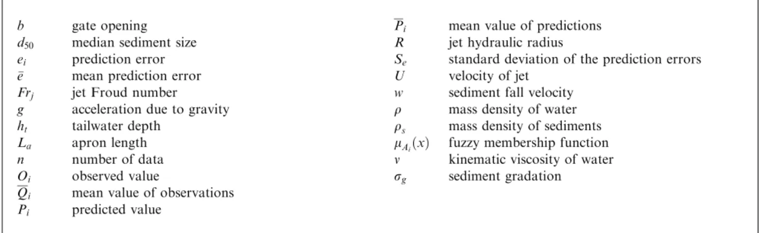
MLP models. As a result, the MLP model having 4 hidden neurons in hidden layer was selected as the best fit model for scour depth prediction.Fig. 3shows the results with the per-formance indices between predicted and observed data for the training and testing data sets, respectively.Fig. 3 shows that the MLP model performance is accurate and reliable.
As can be seen fromFig. 3b, the MLP model underestimates
the maximum scour depth for test data.
3.4. ANFIS model
In the ANFIS model, fuzzy subtractive clustering algorithm was used to design an initial rule base. The objective of the fuzzy subtractive clustering was to prevent increasing numbers
of parameters which may be altered according to the number of rules. The genfis2 function generates a model from data using clustering and requires a specified cluster radius. Specify-ing a small cluster radius usually yields many small clusters in the data hence resulting in many rules. Specifying a large clus-ter radius usually yields a few large clusclus-ters in the data which results in fewer rules. Cluster size 0.5 was chosen for the test as it shows a satisfaction of training and testing result. A combi-nation of least-squares method and back-propagation algo-rithm (hybrid model) is used to optimize the function parameters.
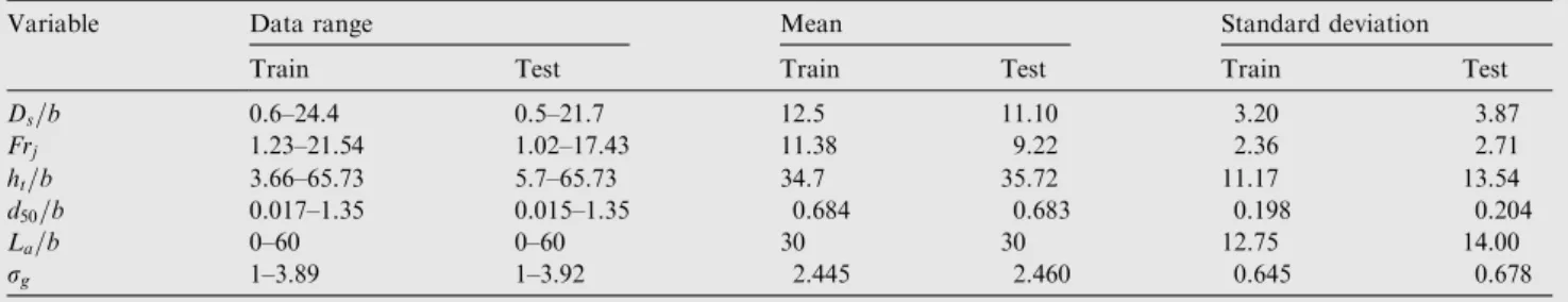
To evaluate the performance of the ANFIS model, observed dimensionless scour depth values are plotted against
Figure 3 Plot of observed and predicted scour depth with original data set using ANN model (a) training and (b) test.
the predicted ones.Fig. 4 shows the results with the perfor-mance indices between predicted and observed data for the training and testing data sets, respectively. As can be seen from
Fig. 4ANFIS has performed well in predicting the dimension-less scour depth.
3.5. SVR model
Fig. 5provides the graph plotted between observed and pre-dicted value of dimensionless scour depth obtained by using RBF kernel based SVR with the train and test data. As can
be seen fromFig 5b, the SVR model overestimates the
maxi-mum scour depth for test data.
3.6. GEP model
The chromosomal architecture including number of chromo-somes (30-50-100), head size 4-7) and number of genes (2-3-5) were selected and different combination of the mentioned parameters was tested. The model was run for number of gen-erations and was stopped when there was no significant change in the fitness function value and coefficient of correlation. After some trials, it was found that after 40,000 generations, there was no appreciable change. Parameters of the optimized
GEP model are shown inTable 4.
The explicit formulations of GEP for non-dimensional scour depth prediction as a function of Uffiffiffiffi
gb p ;La b; d50 b ; ht b;rgwere obtained as follows:
Figure 4 Plot of observed and predicted scour depth with original data set using ANFIS model (a) training and (b) test.
Figure 5 Plot of observed and predicted scour depth with original data set using SVR model (a) training and (b) test.
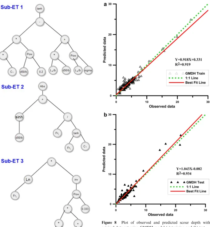
Ds b ¼a1þa2þa3 ð20Þ a1¼tanh 2:75Frj d50 b 1=5! La b d50 b þr La b g " # ð21Þ a2¼ sinh d50 b þ Frj tanhðFrj8:689Þ ð22Þ a3¼lnðFrjÞ 1 1:51d50b La b þrg 1=3 " # ð23Þ
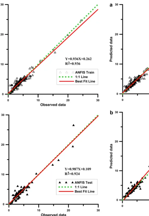
Fig. 6 provides the graph plotted between observed and predicted value of dimensionless scour depth obtained by using
GEP model with the train and test data set.Fig. 7shows the
expression trees of the aforesaid formulation.
3.7. GMDH Neural Network
A two-variable quadratic polynomial function was used in this study. Back propagation algorithm used to train the network.
Fig. 8provides the graph plotted between observed and pre-dicted value of dimensionless scour depth obtained by using GMDH Neural Network with the train and test data set.
3.8. Comparison soft-computing methods and empirical equations
To assess the performance of different soft-computing meth-ods, results of the soft-computing methods are compared with empirical models.Table 5 indicates the statistical parameters for different models for test and train data set. According to
Table 5, almost all of the soft-computing techniques perform better than regression and empirical based models for test data. ANN model is the best model for prediction of dimen-sionless scour depth (RMSE¼0:839, R2¼0:955 for train data andRMSE¼0:869,R2¼0:937 for test data. The second
best model is GEP model (RMSE¼0:761, R2¼0:962 for
train data andRMSE¼0:957,R2¼0:961 for test data. After GEP model, GMDH, ANFIS and SVM models estimate the
maximum scour depth by RMSE= 0.964, 0.971 and 1.175
respectively. ANFIS, GMDH and SVM models overestimate
the maximum scour depth for test data (MBE=0.052,
0.01 and0.231 respectively), while ANN and GEP models
underestimate it (MBE= 0.076 and 0.015 respectively). The
main advantage of the GEP model is an algebraic equation
Figure 6 Plot of observed and predicted scour depth with original data set using GEP model (a) training and (b) test. Table 4 Parameters of the optimized GEP model.
Parameters Definition Value
P1 Function set +,,,,xn,powðx;yÞ, sinh, tanh, Ln, Inv
P2 Mutation rate 0.044
P3 Inversion rate 0.1
P4 One-point recombination rate 30%
P5 Two-point recombination rate 30%
P6 Gene recombination rate 0.1
P7 Gene transposition rate 0.1
P8 Linking function Addition
that can be used easily for practical applications. The GMDH model predicts the values of dimensionless scour depth by
RMSE¼0:799, R2¼0:958 for train data and
RMSE¼0:964,R2¼0:966 for test data.
As can be seen fromTable 5, the equation suggested by Dey
and Sarkar[2] (RMSE= 1.048,R2= 0.937) provides better
estimation than other empirical equations. Linear and nonlin-ear regression equations (Eqs.(18) and (19)) proposed in the present study could not increase the accuracy of Dey and
Sarkar[2]equation (RMSE= 1.266 for linear regression and
RMSE= 2.324 for nonlinear regression). Empirical equations
suggested by Melville and Lim[1], Lim and Yu[11]and
Chat-terjee et al. [7] had lower accuracy (RMSE= 3.419,
RMSE= 2.136 and RMSE= 2.278 respectively). Dey and
Sarkar[2], Lim and Yu[11]and Melville and Lim[1]equations
overestimate the maximum scour depth (MBE=0.417,
0.851 and 2.525 respectively), while Chatterjee et al. [7]
underestimate the maximum scour depth (MBE= 1.457).
Melville and Lim [1] equation had the worst accuracy and
mean averaged percentage error (MAPE) was about 80%.
Thus, in comparison with other models and equations, appli-cation of this equation is not recommended.
Figure 7 GEP expression tree.
Figure 8 Plot of observed and predicted scour depth with original data set using GMDH model (a) training and (b) test.
3.9. Sensitivity analysis
To evaluate the significance of input variables on maximum scour depth, sensitivity analysis was performed on the ANN model due to minimum error of it. In the analysis, one
parameter of Eq. (3)was eliminated each time to assess its
affection to the output. In this way, theRMSEvalues are char-acterized as common statistical errors. Results of sensitivity analysis are presented inTable 6. Accordingly, the jet Froude number (Frdj) was found to be the most effective parameter
(R2= 0731, RMSE= 1.793) on the prediction of maximum
scour depth, While the apron length ratio (La=b) was found
to be the least effective parameter on the prediction of
maximum scour depth. Aderibigbe and Rajaratnam[4] also
showed that the scour depth is primarily a function of the jet densimetric Froude number.
4. Conclusion
In this paper an attempt was made to determine the best method for estimating maximum scour depth issuing from a sluice gate. The results of the ANN, ANFIS, SVR and GEP methods had good agreements with the measured experimental data. Also the results of these models were compared with the existing empirical [1,2,7,11] and regression based equations. Data sets for performing the training and testing stages were
gathered from literatures [2,4,7]. It was shown that the
ANN, SVR, ANFIS, GMDH and GEP models had less com-putational errors than the empirical equations. Moreover results showed that soft computing models are superior to regression models (linear and nonlinear). The rank of soft computing models according to root mean square error was
ANN, GEP, GMDH, ANFIS and SVM (RMSE= 0.869,
0.957, 0.964, 0.971 and 1.175 respectively). Comparing GEP and ANN methods, derived equation from GEP is more appli-cable than the black box approach of ANN; however, the accuracy of ANN model was slightly higher than GEP model.
Between the traditional equations, Dey and Sarkar [2]
equa-tion had relatively low errors (RMSE= 1.048 and
MAPE= 36.9%) in comparison with other equations.
Mel-ville and Lim [1] equation did not yield satisfactory results
for data set of the present study (RMSE= 3.419 and
MAPE= 80.4%). Additionally, sensitivity analysis is
per-formed and it is found that Jet Froude number is the most effective parameter on maximum scour depth downstream of a sluice gate. On the other hand, apron length ratio is the least effective parameter on maximum scour depth. For the future researchers it is proposed that meta-heuristic optimization techniques such as particle swarm optimization (PSO) and arti-ficial bee colony (ABC) are applied for training process of soft computing techniques.
References
[1] Melville B, Lim S. Scour caused by 2D horizontal jets. J Hydraul Eng 2014;140(2):149–55.
[2] Dey S, Sarkar A. Scour downstream of an apron due to submerged horizontal jets. J Hydraul Eng 2006;132(3): 246–57.
[3] Valentin F. Considerations concerning scour in the case of flow under gates; 1967.
[4] Aderibigbe O, Rajaratnam N. Effect of sediment gradation on erosion by plane turbulent wall jets. J Hydraul Eng 1998;124 (10):1034–42.
[5] Ali K, Lim S. Local scour caused by submerged wall jets. In: ICE Proceedings. Thomas Telford; 1986.
[6] Altinbilek HD, Basmaci Y. Localized scour at the downstream of outlet structures. In: Proc. 11th congress on large dams. [7] Chatterjee S, Ghosh S, Chatterjee M. Local scour due to
submerged horizontal jet. J Hydraul Eng 1994;120(8):973–92. [8] Farhoudi J, Smith KV. Time scale for scour downstream of
hydraulic jump. J Hydraul Div 1982;108(10):1147–62.
[9] Hamidifar H, Omid M, Nasrabadi M. Scour downstream of a rough rigid apron. World Appl Sci J 2011;14(8):1169–78. [10] Hopfinger EJ et al. Sediment erosion by Go¨rtler vortices: the
scour-hole problem. J Fluid Mech 2004;520:327–42.
[11] Lim S, Yu G. Scouring downstream of sluice gate. In: First international conference on scour of foundations.
[12] Verma DVS, Goel A. Scour downstream of a sluice gate. ISH J Hydraul Eng 2005;11(3):57–65.
Table 6 Sensitivity analysis for input parameters with ANN model. Function R2 (train) RMSE (train) R2 (test) RMSE (test) Ds b ¼w pUffiffiffiffigb; La b; d50 b; ht b 0.892 0.924 0.908 1.549 Ds b ¼w La b; d50 b ; ht b;rg 0.527 2.029 0.731 1.793 Ds b ¼w Uffiffiffiffi gb p ;d50 b ; ht b;rg 0.919 0.806 0.885 1.444 Ds b ¼w pUffiffiffiffigb; La b; d50 b;rg 0.865 1.521 0.843 1.621 Ds b ¼w Uffiffiffiffi gb p ;La b; ht b;rg 0.844 1.124 0.857 1.333 Bold values are best results.
Table 5 Performance of different models for train and test data sets.
Model RMSE MBE MAPE % MAE R2 ANN (test) 0.869 0.076 18.842 0.615 0.968 SVM (test) 1.175 0.231 15.78 0.601 0.968 ANFIS (test) 0.971 0.052 19.42 0.626 0.971 GEP (test) 0.957 0.015 20.04 0.602 0.961 GMDH (test) 0.964 0.010 17.94 0.621 0.966 ANN (train) 0.839 0.085 20.67 0.599 0.955 SVM (train) 0.661 0 17.52 0.469 0.972 ANFIS (train) 0.711 0 19.25 0.509 0.967 GEP (train) 0.761 0.011 20.14 0.538 0.962 GMDH (train) 0.799 0 21.51 0.594 0.958 Nonlinear multiple regression 2.324 0.768 43.73 1.307 0.832 Linear multiple regression 1.266 0.449 29.386 0.955 0.938 Melville and Lim[1] 3.419 2.525 80.471 2.541 0.925 Dey and Sarkar[2] 1.048 0.417 36.919 0.727 0.937 Lim and Yu[11] 2.136 0.851 37.607 1.172 0.915 Chatterjee et al.[7] 2.278 1.457 34.313 1.594 0.896 Bold values are best results.
[13]Balachandar R, Kells JA, Thiessen RJ. The effect of tailwater depth on the dynamics of local scour. Can J Civ Eng 2000;27 (1):138–50.
[14]Farhoudi J, Smith KVH. Local scour profiles downstream of hydraulic jump. J Hydraul Res 1985;23(4):343–58.
[15]Balachandar R, Kells JA. Instantaneous water surface and bed scour profiles using video image analysis. Can J Civ Eng 1998;25 (4):662–7.
[16]Balachandar R, Kells JA. Local channel in scour in uniformly graded sediments: the time-scale problem. Can J Civ Eng 1997;24 (5):799–807.
[17]Najafzadeh M, Lim S. Application of improved neuro-fuzzy GMDH to predict scour depth at sluice gates. Earth Sci Inf 2014:1–10.
[18]Ayoubloo MK, Etemad-Shahidi A, Mahjoobi J. Evaluation of regular wave scour around a circular pile using data mining approaches. Appl Ocean Res 2010;32(1):34–9.
[19]Azamathulla HM, Deo MC, Deolalikar PB. Alternative neural networks to estimate the scour below spillways. Adv Eng Softw 2008;39(8):689–98.
[20]Bateni SM, Borghei SM, Jeng DS. Neural network and neuro-fuzzy assessments for scour depth around bridge piers. Eng Appl Artif Intell 2007;20(3):401–14.
[21]Bateni SM, Jeng D-S, Melville BW. Bayesian neural networks for prediction of equilibrium and time-dependent scour depth around bridge piers. Adv Eng Softw 2007;38(2):102–11.
[22]Etemad-Shahidi A, Yasa R, Kazeminezhad MH. Prediction of wave-induced scour depth under submarine pipelines using machine learning approach. Appl Ocean Res 2011;33(1):54–9. [23]Firat M, Gungor M. Generalized regression neural networks and
feed forward neural networks for prediction of scour depth around bridge piers. Adv Eng Softw 2009;40(8):731–7.
[24]Ismail A et al. Predictions of bridge scour: application of a feed-forward neural network with an adaptive activation function. Eng Appl Artif Intell 2013;26(5–6):1540–9.
[25]Kaya A. Artificial neural network study of observed pattern of scour depth around bridge piers. Comput Geotech 2010;37 (3):413–8.
[26]Lee TL et al. Neural network modeling for estimation of scour depth around bridge piers. J Hydrodyn Ser B 2007;19(3): 378–86.
[27]Moussa YAM. Modeling of local scour depth downstream hydraulic structures in trapezoidal channel using GEP and ANNs. Ain Shams Eng J 2013;4(4):717–22.
[28]Onen F. Prediction of scour at a side-weir with GEP, ANN and regression models. Arab J Sci Eng 2014;39(8):6031–41.
[29]Ghazanfari-Hashemi S et al. Prediction of pile group scour in waves using support vector machines and ANN. J Hydroinform 2011;13(4):609–20.
[30]Farhoudi J, Hosseini SM, Sedghi-Asl M. Application of neuro-fuzzy model to estimate the characteristics of local scour down-stream of stilling basins. J Hydroinform 2010;12(2):201–11. [31]Akib S, Mohammadhassani M, Jahangirzadeh A. Application of
ANFIS and LR in prediction of scour depth in bridges. Comput Fluids 2014;91:77–86.
[32]Azamathulla HM, Ghani AAb, Fei SY. ANFIS-based approach for predicting sediment transport in clean sewer. Appl Soft Comput 2012;12(3):1227–30.
[33]Bateni SM, Jeng DS. Estimation of pile group scour using adaptive neuro-fuzzy approach. Ocean Eng 2007;34(8–9):1344–54. [34]Keshavarzi A, Gazni R, Homayoon SR. Prediction of scouring around an arch-shaped bed sill using neuro-fuzzy model. Appl Soft Comput 2012;12(1):486–93.
[35]Zounemat-Kermani M et al. Estimation of current-induced scour depth around pile groups using neural network and adaptive neuro-fuzzy inference system. Appl Soft Comput 2009;9(2): 746–55.
[36]Najafzadeh M, Etemad-Shahidi A, Lim SY. Scour prediction in long contractions using ANFIS and SVM. Ocean Eng 2016;111:128–35.
[37]Firat M. Scour depth prediction at bridge piers by Anfis approach. Proc Inst Civ Eng – Water Manage 2009;162(4): 279–88.
[38]Firat M, Gu¨ngo¨r M. Monthly total sediment forecasting using adaptive neuro fuzzy inference system. Stoch Environ Res Risk Assess 2009;24(2):259–70.
[39]Goel A, Pal M. Application of support vector machines in scour prediction on grade-control structures. Eng Appl Artif Intell 2009;22(2):216–23.
[40]Hong J-H et al. Predicting time-dependent pier scour depth with support vector regression. J Hydrol 2012;468–469:241–8. [41]Goyal MK, Ojha CSP. Estimation of scour downstream of a
ski-jump bucket using support vector and M5 model tree. Water Resour Manage 2011;25(9):2177–95.
[42]Etemad-Shahidi A, Ghaemi N. Model tree approach for predic-tion of pile groups scour due to waves. Ocean Eng 2011;38 (13):1522–7.
[43]Samadi M, Jabbari E, Azamathulla HM. Assessment of M50 model tree and classification and regression trees for prediction of scour depth below free overfall spillways. Neural Comput Appl 2012;24(2):357–66.
[44]Pal M, Singh NK, Tiwari NK. M5 model tree for pier scour prediction using field dataset. KSCE J Civ Eng 2012;16 (6):1079–84.
[45]Guven A, Gunal M. Genetic programming approach for predic-tion of local scour downstream of hydraulic structures. J Irrig Drain Eng 2008;134(2):241–9.
[46]Azamathulla HMd et al. Genetic programming to predict ski-jump bucket spill-way scour. J Hydrodyn Ser B 2008;20 (4):477–84.
[47]Azamathulla HMd et al. Genetic programming to predict bridge pier scour. J Hydraul Eng 2009;136(3):165–9.
[48]Azamathulla HM, Guven A, Demir YK. Linear genetic program-ming to scour below submerged pipeline. Ocean Eng 2011;38(8– 9):995–1000.
[49]Guven A, Azamathulla HM, Zakaria NA. Linear genetic programming for prediction of circular pile scour. Ocean Eng 2009;36(12–13):985–91.
[50]Azamathulla H, Yusoff MAMohd. Soft computing for prediction of river pipeline scour depth. Neural Comput Appl 2013;23(7– 8):2465–9.
[51]Najafzadeh M. Neuro-fuzzy GMDH based particle swarm optimization for prediction of scour depth at downstream of grade control structures. Eng Sci Technol Int J 2015(0). [52]Najafzadeh M, Barani GA. Comparison of group method of data
handling based genetic programming and back propagation systems to predict scour depth around bridge piers. Sci Iran 2011;18(6):1207–13.
[53]Najafzadeh M, Barani G-A, Azamathulla HM. GMDH to predict scour depth around a pier in cohesive soils. Appl Ocean Res 2013;40:35–41.
[54]Najafzadeh M, Barani G-A, Hessami Kermani MR. GMDH based back propagation algorithm to predict abutment scour in cohesive soils. Ocean Eng 2013;59:100–6.
[55]Najafzadeh M, Barani G-A, Hessami-Kermani M-R. Evaluation of GMDH networks for prediction of local scour depth at bridge abutments in coarse sediments with thinly armored beds. Ocean Eng 2015;104:387–96.
[56]Najafzadeh M, Azamathulla HM. Neuro-fuzzy GMDH to predict the scour pile groups due to waves. J Comput Civ Eng 2015;29 (5):04014068.
[57]Najafzadeh M. Neurofuzzy-based GMDH-PSO to predict max-imum scour depth at equilibrium at culvert outlets. J Pipeline Syst Eng Pract 2016;7(1):06015001.
[58]Najafzadeh M, Barani G-A, Hessami-Kermani M-R. Group method of data handling to predict scour at downstream of a ski-jump bucket spillway. Earth Sci Inf 2014;7(4):231–48.
[59]Najafzadeh M. Neuro-fuzzy GMDH systems based evolutionary algorithms to predict scour pile groups in clear water conditions. Ocean Eng 2015;99:85–94.
[60]Rajaratnam N. Erosion by plane turbulent jets. J Hydraul Res 1981;19(4):339–58.
[61]Tabari H et al. SVM, ANFIS, regression and climate based models for reference evapotranspiration modeling using limited climatic data in a semi-arid highland environment. J Hydrol 2012;444–445:78–89.
[62]Bilgili M. Prediction of soil temperature using regression and artificial neural network models. Meteorol Atmos Phys 2010;110 (1–2):59–70.
[63]Araghinejad S. Data-driven modeling: using MATLAB in water resources and environmental engineering. Springer; 2014. [64]Wang W-C et al. A comparison of performance of several artificial
intelligence methods for forecasting monthly discharge time series. J Hydrol 2009;374(3–4):294–306.
[65]Hykin S. Neural networks: a comprehensive foundation. New Jersey: Printice-Hall. Inc.; 1999.
[66]Vapnik V. The nature of statistical learning theory. Springer; 1995.
[67]Jang JSR. ANFIS: adaptive-network-based fuzzy inference sys-tem. IEEE Trans Syst Man Cybernet 1993;23(3):665–85. [68] Ferreira C. Gene expression programming: a new adaptive
algorithm for solving problems. arXiv: preprint cs/0102027; 2001. [69]Koza JR. Genetic programming: on the programming of
com-puters by means of natural selection, vol. 1. MIT press; 1992. [70]Ferreira C. Gene expression programming. Berlin: Springer; 2006. [71]Zakaria NA et al. Gene expression programming for total bed material load estimation—a case study. Sci Total Environ 2010;408(21):5078–85.
[72]Garg V. Inductive group method of data handling neural network approach to model basin sediment yield. J Hydrol Eng 2014;20(6): C6014002.
[73] Nariman-zadeh N et al. Modelling of explosive cutting process of plates using GMDH-type neural network and singular value decomposition. J Mater Process Technol 2002;128(1–3):80–7. [74] Kalantary F, Ardalan H, Nariman-Zadeh N. An investigation on
the Su–NSPT correlation using GMDH type neural networks and genetic algorithms. Eng Geol 2009;104(1–2):144–55.
[75] Witczak M et al. A GMDH neural network-based approach to robust fault diagnosis: application to the DAMADICS bench-mark problem. Control Eng Pract 2006;14(6):671–83.
Dr. Masoud Karbasiis Assistant Professor in Department of water engineering, Faculty of Agriculture, University of Zanjan, Islamic Republic of Iran, He graduated in irrigation Engineering from the Urmia University in 2003 and post graduated in Hydraulic Struc-ture from University of Tehran in 2005. He completed his PhD in Hydraulic Structures from University of Tehran in 2011. He has published 4 Journal papers; presented more than 15 conferences papers. His interest research is hydraulics of sediment transport, river engineering and hydraulic structures.
Dr. H.Md. Azamathullais Associate Professor in Department of civil engineering, Faculty of Engineering, University of Tabuk, Saudi Arabia, He graduated in Civil Engineering from the S. K. D., University, Ananthapur in 1994 and post graduated from SGSITS, Devi Ahilya University, Indore in 1997. He com-pleted his PhD from Indian Institute of Technology, Bombay in 2005.