Low-complexity supervised learning for gesture and shape recognition

(1)

Low-Complexity Supervised Learning for

Gesture and Shape Recognition

A thesis submitted to the

Graduate School of Natural and Applied Sciences

by

Sait Celebi

in partial fulllment for the degree of Master of Science

in

(2)

in scope and quality, as a thesis for the degree of Master of Science in Electronics and Computer Engineering.

APPROVED BY:

Assist. Prof. Tark Arc . . . . (Thesis Advisor)

Assist. Prof. Ahmet Bulut . . . . Assist. Prof. Bu§ra Gedik . . . .

This is to conrm that this thesis complies with all the standards set by the Graduate School of Natural and Applied Sciences of stanbul ehir University:

DATE OF APPROVAL: 20 February 2014

(3)

Declaration of Authorship

I, Sait Celebi, declare that this thesis titled, 'Low-Complexity Supervised Learning for Gesture and Shape Recognition' and the work presented in it are my own. I conrm that:

This work was done wholly or mainly while in candidature for a research degree at

this University.

Where any part of this thesis has previously been submitted for a degree or any

other qualication at this University or any other institution, this has been clearly stated.

Where I have consulted the published work of others, this is always clearly

at-tributed.

Where I have quoted from the work of others, the source is always given. With the

exception of such quotations, this thesis is entirely my own work.

I have acknowledged all main sources of help.

Where the thesis is based on work done by myself jointly with others, I have made

clear exactly what was done by others and what I have contributed myself.

Signed:

Date: 20 February 2014

(4)

else we do.

(5)

Low-Complexity Supervised Learning for Gesture and Shape

Recognition

Sait Celebi

Abstract

Classication is a machine learning task in which the objective is to categorize given samples according to their attributes. Gesture Recognition (GR) and Shape Recognition (SR) are two classication examples. Some daily-life applications of these include Hand Gesture Recognition (HGR) and Optical Character Recognition (OCR).

GR is a challenging classication problem often used in human-computer interaction applications to provide a natural interface between user and computer. Since the same gesture might be performed with dierent speeds, Dynamic Time Warping (DTW) is needed to nd the optimal alignment between two time sequences. Oftentimes a pre-processing of sequences is required to remove variations between the reference gestures and the test gestures. We discuss a set of pre-processing methods to make the gesture recognition mechanism robust to these variations. DTW computes a dissimilarity mea-sure by time-warping the sequences on a per sample basis by using the distance between the current reference and test sequences. However, all body joints involved in a gesture are not equally important in computing the distance between two sequence samples. We propose a weighted DTW method that weights joints by optimizing a discriminant ratio. SR is another classication problem with increasing number of applications from OCR to pedestrian detection. Decision tree is a good choice of classier for shape recognition because it is easy to implement and visualize and has lower computational complexity. Bagging randomized decision trees as random forests increases the accuracy rates if the trees are weakly correlated. We propose using random rectangles in combination with random forests and test our method on OCR and GR datasets. We show that the accuracy of our method is similar to the OCR state-of-the-art and better than the GR state-of-the-art, while executing signicantly faster, which makes our proposed method a good t for real-time object/shape recognition. Then discuss how a simple feature such as a random rectangle can perform similar to the complex statistical and structural features designed for shape recognition. Finally we analyze the eect of our parameters. Keywords: Gesture Recognition, Dynamic Time Warping, Kinect, Shape Recognition, Random Forests, Decisin Trees

(6)

Sait Celebi

Öz

Snandrma, verilen örnekleri özelliklerini kullanarak kategorize etme i³ini yapan makine ö§renmesi görevidir. Hareket Alglama (HA) ve ekil Alglama (A) iki adet snandrma örne§idir. El Hareketlerini Alglama (EHA) ve Optik Karakter Tanma (OKT) bu alan-lardaki günlük hayatta kar³la³lan baz uygulamalardr.

EHA, genellikle insan-bilgisayar etkile³imi uygulamalarnda kullanlan, insan ve bilgisa-yar arasnda do§al bir arayüz sunan zor bir snandrma problemidir. Ayn el hareketi farkl hzlarda uygulanabilece§i için, Dinamik Zaman Bükmesi (DZB) iki tane zaman dizisi arasndaki en iyi uyu³may bulmak için kullanlr. Ço§u zaman referans ve test örneklerindeki farkllklardan dolay bir ön-i³leme mekanizmas gereklidir. Hareket tan-mann bu tip farkllklardan ba§msz olarak iyi çal³abilmesi için birkaç ön-i³leme metodu gereklidir. DZB, hali hazrda bulunan test örne§iyle tüm referans örneklerini tek tek tüm parçalarn uyu³turmaya çal³arak bir farkllk ölçütü hesaplar. Fakat bir el hareketini al-glarken vücudun tüm parçalarnn a§rl§ e³it de§ildir. Bu çal³mada vücut parçalarn bir farkllk orann optimize ederek a§rlaklandrmay öneriyoruz. Son olarak, ön-i³leme ve a§rlklandrma yöntemlerimizi klasik DZB ve tekni§in bilinen en iyi durumu ile kyaslyoruz.

A, OKT'den yaya alglamaya kadar uzanan artan sayda uygulamalara sahip di§er bir snandrma problemidir. Karar a§açlar uygulamas kolay oldu§u için, görselle³tir-ilebilmesi mümkün oldu§u için ve hesaplama kar³kl§ az oldu§u A için uygun bir snandrc seçimidir. E§er snandrma için birden fazla birbiriyle az ili³kili karar a§ac beraber kullanlyorsa (rastgele orman) snandrma kalitesi artar. Bu çal³mada rastgele orman snandrclarn resimlerden rastgele seçti§imiz dikdörtgen özellikleriyle kullanyoruz. Metodumuzu karakter tanma ve hareket tanma datasetleriyle test ediy-oruz. Görülüyor ki bu yöntem ³uana kadar bilinen en iyi yöntemlerle yakla³k do§rulukta çal³maktadr. Bunun yannda bunlara kyasla çok daha hzl çal³maktadr ki bu özelli§i bu yöntemi gerçek zamanl nesne ve ³ekil tanma uygulamalarna uygun klmaktadr. Rastgele dikdörtgenler gibi basit tanmlayclarn kar³k istatistiksel ve yapsal tanm-layclara göre ne kadar da ³a³rtc ³ekilde iyi çal³t§ üzerine tart³yoruz. Son olarak da sistemde kulland§mz parametreleri analiz ediyoruz.

Anahtar Sözcükler: Hareket Tanma, Dinamik Zaman Bükmesi, Kinect, ekil Tanma, Rastgele Orman, Karar A§açlar

(7)

This thesis is lovingly dedicated to my mother for her constant love

to me throughout my life.

(8)

I would like to express my sincere gratitude to my advisor Prof. Tarik Arici for his con-tinuous support, motivation, enthusiasm, and time. His guidance helped me throughout the duration of the research conducted and the writing of this thesis.

Besides my advisor, I would like to thank to the rest of my thesis committee: Prof. Ahmet Bulut and Prof. Bugra Gedik for their helpful and constructive comments. I thank my fellow lab-mates in Istanbul Sehir University, Data Science Group: Ali Selman Aydin, Erkan Bilmez and Talha Tarik Temiz for the sleepless nights we were working together before deadlines, and for all the fun we have had in the last two years.

Also, I would like to thank all Sehir University members who participated in our ges-ture database recordings and patiently performed all the gesges-tures that helped in our experiments.

Most importantly, I would like to thank my family, for their constant support without knowing a bit what I was doing on my thesis at the time.

(9)

List of Figures

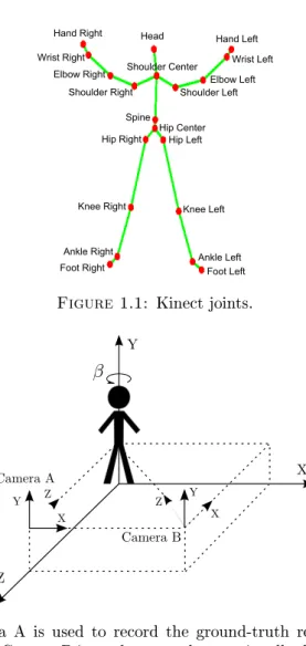
1.1 Kinect joints. . . 4

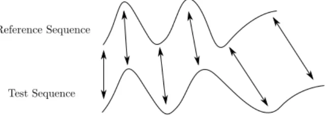
1.2 Camera A is used to record the ground-truth reference gestures with per-pendicular angles, Camera B is used to record a rotationally distorted test sequence. β is the desired angle to rotate the skeleton in Y axis. After this rotation, the skeleton will be rotated in other axes if needed until it will be perpendicular to all axes. . . 4

1.3 Two skeletons with dierent orientations (Left: Ground-truth reference frame, Right: Rotationally distorted test frame due to improper body orientation) . . . 5

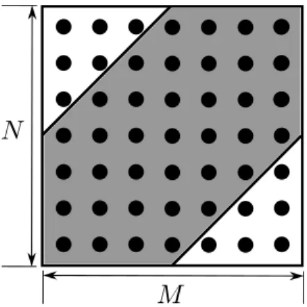
1.4 DTW used to match two sequences, reference sequence and test sequence. 5 1.5 Accumulated cost matrix of two sequencesRandT with sizesN andM, respectively. Global constraint region, R, Sakoe-Chiba band [49], is shown with gray color. . . 7

1.6 Predecessor nodes used in Bellman's principle where nl ∈ [1 :N], ml ∈ [1 :M] and l ∈[2 : L]. Note that(nl−1, ml−1) ∈ {(nl−1, ml),(nl, ml− 1),(nl−1, ml−1)}. . . 8

1.7 Two sample reference gestures in the gesture database: Right Hand Push Up and Left Hand Wave. . . 10

1.8 Discriminant ratios for with and without pre-processed gesture samples using the rotationally distorted gesture database. Note that the discrimant ratios are increased, on average, 42% with the proposed pre-processing method. There are 21 gesture samples in each gesture class. The gesture classes are, namely, Both Hands Pull Down, Both Hands Push Up, Left Hand Pull Down, Left Hand Push Up, Left Hand Swipe Left, Left Hand Swipe Right, Left Hand Wave, Right Hand Pull Down, Right Hand Push Up, Right Hand Swipe Left, Right Hand Swipe Right, Right Hand Wave, respectively. . . 13

2.1 An example data instance . . . 19

2.2 Univariate decision tree . . . 20

2.3 Multivariate decision tree . . . 20

2.4 Example Viola-Jones features relative to the detection window. The sum of the pixel intensities in the grey rectangular regions are subtracted from the white rectangular regions. . . 24

2.5 Cascaded application of classiers enable focusing on object-like regions. . 24

(11)

List of Figures x 2.6 Visualization of a decision tree up to the fourth depth level trained on

OCR data. The thickness of the edges connecting nodes is proportional to the number of images associated with the receiving node. The average of all training images at a node is displayed. The brightness of the circle below the average image is inversely proportional to the entropy at that

node: the higher the entropy the darker the color of the circle. . . 26

2.7 Sample digits from the MNIST database . . . 29

2.8 Accuracy as the number of trees is increased . . . 31

2.9 The eect of the number of candidate rectangles per each split node . . . 31

2.10 Accuracy versus maximum tree depth using a random forest of ve ran-domized trees. . . 32

2.11 Average per-tree accuracy versus maximum tree depth . . . 33

2.12 Accuracy versus number of trees using dierent features . . . 33

(12)

List of Tables

1.1 Confusion matrix for the conventional DTW. . . 13 1.2 Confusion matrix for the weighted DTW in [47]. . . 14 1.3 Confusion matrix for our proposed weighted DTW. . . 14 1.4 Accuracies of the three methods. Note that not only six gesture classes

given in Table 1.1, 1.2, and 1.3 are used, but all eight gesture classes are taken into consideration. . . 14 1.5 Overall performance comparison using the rotationally distorted and

re-laxed gesture database. . . 15 2.1 Classication times (milliseconds) on an example image of size28×28. . . 30

2.2 Classication accuracies on the MNIST test set. . . 31 2.3 Gesture recognition accuracies . . . 35

(13)

Chapter 1

Robust Gesture Recognition Using

Feature Pre-Processing and

Weighted Dynamic Time Warping

1.1 Introduction

Interacting with computers using human motion is commonly employed in human-computer interaction (HCI) applications. One way to incorporate human motion into HCI applica-tions is to use a predened set of human joint moapplica-tions i.e., gestures. Gesture recognition has been an active research area [20, 32, 47, 66], and involves state-of-the-art machine learning techniques in order to work reliably in dierent environments. A variety of methods have been proposed for gesture recognition including Dynamic Time Warping [47], Hidden Markov Models [20], Finite State Machines [23], hidden Conditional Ran-dom Fields (CRFs) [61] and orientation histograms [19]. In addition to these, there are methods employed in gesture recognition that are not view-based. Examples of these are the use of Wii controller (Wiimote) [50] and DataGlove [44].

DTW measures similarity between two time sequences which might be obtained by sam-pling a source with varying samsam-pling rates or by recording the same phenomenon occur-ring with varying speeds [64]. After DTW was introduced in 1960s [10], it has been used in solving dierent problems such as speech recognition to warp speech in time to be able to cope with dierent speaking speeds [2, 41, 49], data mining and information retrieval to deal with time-dependent data [1, 45], curve matching [18], online handwriting recog-nition [59], hand shape classication [28]. In gesture recogrecog-nition, DTW time-warps an observed motion sequence of body joints to pre-stored gesture sequences [16, 28, 46, 62]. Although we present the theory of the general DTW and its implementation issues,

(14)

in this paper we focus more on its application to gesture recognition. Comprehensive surveys about the general DTW algorithm can be found in [40, 52].

The conventional DTW algorithm is basically a dynamic programming algorithm, which uses an iterative update of DTW cost by adding the distance between mapped elements of the two sequences at each iteration step. The distance between two elements is oftentimes the Euclidean distance, which gives equal weights to all dimensions of a sequence sample. However, depending on the problem a weighted distance might perform better in assessing the similarity between a test sequence and a reference sequence. For example in a typical gesture recognition problem, body joints used in a gesture can vary from gesture class to gesture class. Hence, not all joints are equally important in recognizing a gesture. With Microsoft's launch of Kinect in 2010, and release of Kinect SDK in 2011, numerous applications and research projects exploring new ways in human-computer interaction have been enabled. Some examples are gesture recognition [47], touch detection using depth data [65], human pose estimation [25], implementation of real-time virtual xtures [48], real-time robotics control applications [58] and the physical rehabilitation of young adults with motor disabilities [15].

We propose a weighted DTW algorithm that uses a weighted distance in the cost com-putation. The weights are chosen so as to maximize a discriminant ratio based on DTW costs. The weights are obtained from a parametric model which depends on how ac-tive a joint is in a gesture class. The model parameter is optimized by maximizing the discriminant ratio. By doing so, some joints will be weighted up and some joints will be weighted down to maximize between-class variance and minimize within-class vari-ance. As a result, irrelevant joints of a gesture class (i.e., parts that are not involved in a gesture class) will contribute to the DTW cost to a lesser extent, while keeping the between-class variances large.

Our system rst extracts body-joint features from a set of skeleton data that consists of six joint positions, which are left and right hands, wrists and elbows. We have observed that the gestures in our training set, which have quite dierent motion patterns, require the use of all or a subset of these six joints only. These obtained skeleton features are used to recognize gestures by matching them with pre-stored reference sequences. Pre-processing is needed to suppress the noise due to dierent body and camera orientations, and dierent body sizes. After pre-processing is done, the matching is performed by assigning a test sequence to a reference sequence with the minimum DTW cost. By removing the variations in the data, the DTW cost becomes more reliable in classication as demonstrated by the increase in the discriminant ratio values.

(15)

Chapter 1. Gesture Recognition 3

1.2 Related Work

One commonly used technique for gesture recognition is using HMMs for modeling ges-ture sequences. HMMs are especially known for their application to speech recognition, gesture recognition, bioinformatics, etc. HMMs are statistical models for sequential data [7, 8], and therefore can be used in gesture recognition [20, 30, 57]. The states of an HMM are hidden and state transition probabilities are to be learned from the training data. However, dening states for gestures is not an easy task since gestures can be formed by a complex interaction of dierent joints. Also, learning the model parameters i.e., transition probabilities, requires large training sets, which may not always be available. On the other hand, DTW does not require training but needs good reference sequences to align with.

Using a weighting scheme in DTW cost computation has been proposed for gesture recognition [47]. The method proposed in [47] uses DTW costs to compute between and within class variations to nd a weight for each body joints. These weights are global weights in the sense that there is only one weight computed for a body joint. However, our proposed method computes a weight for each body joint and for each gesture class. This boosts the discriminative power of DTW costs since a joint that is active in one gesture class may not be active in another gesture class. Hence weights has to be adjusted accordingly. This helps especially dealing with within-class variation. To avoid reducing the between-class variance, we compute weights by optimizing a discriminant ratio using a parametric model that depends on body joint activity. In the next section we discuss data acquisition and feature pre-processing.

1.3 Data Acquisition and Feature Pre-processing

We use Microsoft Kinect sensor [53] to obtain joint positions. Kinect SDK tracks 3D coordinates of 20 body joints given in Figure 1.1 in real time (30 frames per second). Since the machine learning algorithm uses depth images to predict joint positions, the skeleton model is quite robust to color, texture, and background.

We have observed that only six out of the 20 joints contribute in identifying a hand gesture: left hand, right hand, left wrist, right wrist, left elbow and right elbow. A feature vector consists of 3D coordinates of these six joints and is of dimension of 18 as given below

(16)

Hand Right Wrist Right Hand Left Wrist Left Elbow Left Elbow Right Head Shoulder Right Foot Right Shoulder Left Foot Left Ankle Left Ankle Right Knee Left Knee Right Hip Left Hip Right Hip Center Spine Shoulder Center

Figure 1.1: Kinect joints.

Figure 1.2: Camera A is used to record the ground-truth reference gestures with perpendicular angles, Camera B is used to record a rotationally distorted test sequence.

β is the desired angle to rotate the skeleton inYaxis. After this rotation, the skeleton will be rotated in other axes if needed until it will be perpendicular to all axes.

wherenis the index of the skeleton frame at timetn. A gesture sequence is the

concate-nation ofN such feature vectors.

After N feature vectors are concatenated to create the gesture sequence, they are

pre-processed before the DTW cost computation. The pre-processing consists of three stages. First stage is the normalization stage which translates all skeletons to the center of the eld of view. This could be done by subtracting the hip center joint position from the other joint positions. Note that the reference frames are already recorded at the center of the eld of view. The second pre-processing stage removes the rotational distortion caused by dierent orientations of human bodies. Contrary to the reference gestures, where trained performers are used, it is highly possible to have dierent orientations or positionings of users with respect to camera in real-life cases. Such occasions are problematic for gesture recognition since they will result in rotationally distorted skeleton frames. To cope with these occasions, our pre-processing system rotates the skeleton frames if necessary, such that the skeleton frames will be orthogonal to the principal axis

(17)

Figure 1.3: Two skeletons with dierent orientations (Left: Ground-truth reference frame, Right: Rotationally distorted test frame due to improper body orientation)

Figure 1.4: DTW used to match two sequences, reference sequence and test sequence.

of the camera. To this end, we dene two vectors by using spatial coordinates of the right shoulder, left shoulder and hip center which are obtained from Kinect sensor. Using these two vectors, we calculate the three angles, α, β, θ, of the skeleton with respect to the

camera's coordinate system, and compute the rotation matricesRα_x,Rβy,Rθz, respectively.

The rotation is then applied using these angles with the appropriate order. See an example rotation inYaxis with Rβy in Figure 1.2. The third and the last pre-processing

stage is the elimination of variations in the feature vectors due to dierent skeleton ratios (broad-shouldered, narrow-shouldered). All feature vectors are normalized with the distance between the left and the right shoulders to account for the variations due to a person's size. Note that the reference sequences are recorded with people who has average skeleton ratios. Next, we present a more detailed discussion on DTW.

1.4 Dynamic Time Warping for Gesture Recognition

DTW is a template matching algorithm to nd the best match for a test pattern out of the reference patterns, where the patterns are represented as a time sequence of features. In Figure 1.4 we show an example matching of two sequences.

LetR={r1, r2, . . . , rN}, N ∈Nand

T = {t1, t2, . . . , tM}, M ∈ N be reference and test sequences (sequence of set of joint

positions in our case), respectively. The objective is to align the two sequences in time via a nonlinear mapping (i.e., warping or alignment). Such a warping path can be illustrated as an ordered set of points as given below

(18)

wherepl = (nl, ml), denotes mapping of rnl to tml. pl ∈[1 :N]×[1 :M]for l∈[1 :L],

where L is the number of mappings. The total cost D of a warping path p between R

andTwith respect to a distance function d(ri, tj),i∈[1 :N]andj ∈[1 :M], is dened

as the sum of all distances between the mapped sequence elements

Dp=

L

X

l=1

d(rnl, tml), (1.2)

where Dp is the total cost of the path p and d(ri, tj) measures the distance between

elements ri and tj. For gesture recognition, distance can be chosen as the distance

between the corresponding joint positions (3D points) of the reference gesture, R, and

the test gesture T.

A mapping can also be viewed as a path on a two-dimensional (2D) grid, also known as the cost matrix, which is of size N ×M (see Figure 1.5), where grid node (ri, tj)

denotes the distance between ri and tj. The node(r1, t1) which starts the alignment by

matching the rst sequence elements is conventionally placed on the left-bottom corner of the grid. Each pathp on the 2D grid (i.e., the cost matrix) is associated with a total

cost Dgiven in Eq. (1.2). Note that among all possible paths, we are mostly interested

in the path which makes the total accumulated cost minimum while satisfying the desired constraints. Hence, optimal path denoted byp∗ is the path with the minimum total cost.

The DTW distance between two sequences is dened by the distance associated with a total costD given in Eq. (1.2) using the optimal path, i.e.:

DTW(R,T) = Dp∗(R,T). (1.3)

The optimal path species the optimal alignment between two sequences and is computed by nding the path that minimizes the total cost. One way to nd the minimum cost path is to test every possible path on the 2D grid from the left-bottom corner to the right-top corner. However, this has exponential complexity. Dynamic programming reduces the complexity by taking advantage of Bellman's principle [9]. Bellman's optimality principle states that the optimal path from the starting grid node (r1, t1) to the ending node

(rN, tM) through an intermediate point(rn, tm) can be expressed as the concatenation

of the optimal path from (r1, t1) to (rn, tm), and the optimal path from (rn, tm) to

(rN, jM). This implies that if we are given the optimal path from (r1, t1)to (rn, tm), we

only need to search for the optimal path from(rn, tm) to(rN, tM)rather than searching

for paths from (r1, t1) to (rN, tM). We will use Bellman's principle in the total cost

(19)

Figure 1.5: Accumulated cost matrix of two sequencesRandTwith sizesN andM,

respectively. Global constraint region, R, Sakoe-Chiba band [49], is shown with gray color.

Some well-known restrictions on the warping path have been proposed to eliminate unre-alistic correspondences between the sequences [40, 49]. The most fundamental constraints which are applied in various topics as well as gesture recognition, are the following: (i) Boundary conditions: p1 = (1,1), pL= (N, M).

(ii) Step size condition: pl+1−pl∈ {(0,1),(1,0),(1,1)}for l∈[1 :L−1].

The boundary conditions require the whole reference sequence to be mapped to the whole test sequence, and can be modied if this is not strictly desired. The step size condition requires that only one element of both sequences can be skipped at each cost computation step of Bellman's principle. Hence, optimal path can progress from a restricted set of predecessor nodes as shown in Figure 1.6. Since all the elements are ordered in time, the set of predecessor nodes are to the left and bottom of a current node.

First, let's dene C(nl, ml)as below

C(nl,ml) = DTW(R(1 :nl),T(1 :ml)). (1.4)

Note that C(N,M) is equal to DTW(R,T). Let's further assume that the total costs

of the optimal paths to three predecessor nodes denoted by (nl−1, ml), (nl, ml −1),

and (nl−1, ml−1) have been computed. Since the(l−1)th position of the path (i.e.,

(nl−1, ml−1)) is restricted to be one of these three nodes on the 2D grid, Bellman's

principle leads to

C(nl,ml) = min{C(nl,ml−1),

C(nl−1,ml),

(20)

Figure 1.6: Predecessor nodes used in Bellman's principle wherenl∈[1 :N],ml∈[1 :

M]andl∈[2 :L]. Note that(nl−1, ml−1)∈ {(nl−1, ml),(nl, ml−1),(nl−1, ml−1)}.

Finally, the minimum cost path aligning two sequences has cost DTW(R,T), and the

test sequence is matched to the reference sequence that has the minimum cost among all reference sequences.

Although Eq. (1.5) outputs the minimum cost between two sequences, it does not output the optimal path. To nd the optimal path, which can be used to map test sequence elements to reference sequence elements, one needs to backtrack the optimal path starting with the nal node. Note that if the boundary condition is satised, i.e., the whole test sequence is mapped to the whole reference sequence, than (nL, mL) = (N, M) and

(n1, m1) = (1,1).

1.4.1 Boosting The Reliability of DTW

Global constraints dene a set of nodes on the 2D grid to be searched for nding the optimal path. Imposing global constraints not only reduces the DTW computational complexity, but also increases the reliability of DTW's dissimilarity measure by omitting unrealistic paths. We used a well-known global constraint region, Sakoe-Chiba band [49] given in Figure 1.5. The Sakoe-Chiba band eectively limits the warping amount, i.e., slowing down or speeding up of a sequence in time. For example a gesture can be performed with dierent speeds in time depending on the performer but it is logical to expect that there is a limit to how slow or how fast a gesture is performed.

Another problem that degrades DTW's reliability in gesture recognition is due to un-known beginning and ending times of gesture samples. A gesture in a test sequence can often begin later or end sooner than the gesture in the reference sequence stored for that gesture class. Boundary conditions assume that all gestures start at the beginning of the sequence and nish at the ending of the sequence. Hence, imposing boundary conditions in such cases decreases the reliability of DTW costs. To boost the reliability, we relaxed

(21)

Chapter 1. Gesture Recognition 9 the boundary conditions by changing the total cost given in Eq. (1.2) as below

Dp=

L

X

l=1

αld(rnl, tml), (1.6)

whereαlis a weight that is equal to 1 everywhere except the regions close to the starting

node (i.e., left-bottom node denoted by(r1, t1)) and the ending node (i.e., right-top node

denoted by (rN, tM)). To infer the proximity of the current node to starting and ending

nodes the length of the path, ||pl||=

q

n2_l +m2_l, is utilized. The distance terms coming

from the beginning and ending of the sequence is weighted down by computingαl from

the below formula

αl=        ||pl|| τ if||pl|| < τ L−||pl|| τ ifL− ||pl|| < τ 1 otherwise, (1.7)

whereL is the length of the longest path andτ is a threshold value.

1.4.2 Weighted DTW

The conventional DTW computes the dissimilarity between two time sequences by align-ing the two sequences based on a sample based distance as in Eq. (1.5). If the sequence samples are multi-dimensional (18 dimensional for the gesture recognition problem), us-ing an Euclidean distance gives equal importance to all dimensions. We propose to use a weighted distance in the cost computation based on how relevant a body joint is to a specic gesture class. The relevancy is dened as the contribution of a joint to the motion pattern of that gesture class. To infer a joint's contribution to a gesture class we compute its total displacement (i.e., contribution) during the performance of that gesture by a trained user:

C_jg =

N

X

n=2

Distj(f_ng₋₁,f_ng), (1.8)

by whereg is the gesture index,j is the joint index andnis the skeleton frame number. Distj₍₎_{computes the displacement of} _j_{th joint's two consecutive coordinates in feature}

vectors f_ng₋₁, andfng. By summing up these consecutive displacements one can nd the

total displacement of a joint in a selected reference gesture.

After the total displacements are calculated, we lter out the noise (e.g, shaking, trem-bling) and threshold them from the bottom and the top. This prevents our parametric weight model to output too high or low weights as given below

(22)

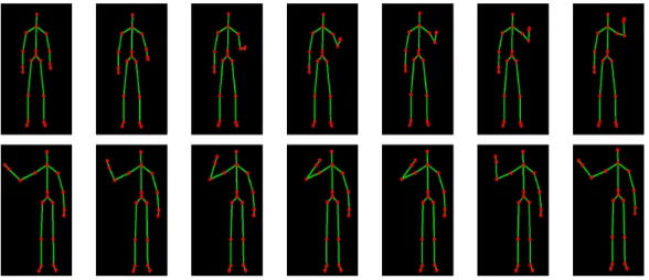
Figure 1.7: Two sample reference gestures in the gesture database: Right Hand Push Up and Left Hand Wave.

C_jg=        Ca if 0≤Cjg < T1 C_jg−T1 T2−T1(Cb−Ca) +Ca if T1 ≤C g j < T2 Cb otherwise, (1.9)

whereCa andCb are threshold values.

Using the total displacement (i.e., contribution) values of joints, the weights of class g

are calculated via

wg_j = 1−e −βC_jg P k 1−e−βCkg , (1.10)

where wg_j is joint j's weight value for gesture class g. Note that in this formulation a

joint's weight value can change depending on the gesture class. For example, for the right-hand-push-up gesture, one would expect the right hand, right elbow and right wrist joints to have large weights, but to have smaller weights for the left-hand-push-up gesture.

To incorporate these weights into the cost, the distance function d(rn, tm) becomes a

weighted average of joints distances between two consecutive frames and is dened to be

d(rn, tm) =

X

j

Distj(rn, tm)wg_j, (1.11)

which gives the distance between nth skeleton frame of reference gesture R and mth

skeleton frame of test gesture T, where R is a sequence known to be in gesture classg

and Tis an unknown test sequence.

The weights are obtained from the model given in Eq. (1.10), which has a single parame-terβ. Our objective is to choose aβvalue that minimizes the within-class variation while

(23)

Chapter 1. Gesture Recognition 11 between-class variation is maximized. Between-class variation maximization and within-class variation minimization can be achieved by making irrelevant joints contribute less to the cost (e.g., reducing the weights of right hand in left-hand-push-up gesture) and not reducing (or possibly increasing) the weights of joints that can help to discriminate dierent gestures. We try to achieve this goal by maximizing a discriminant ratio sim-ilar to Fisher's Discriminant Ratio [27]. To this end, we dene Dg,h(β), as the average

weighted DTW cost between all samples of gesture class g and gesture class h using

weights calculated with given β. Then between-class dissimilarity is the average of all Dg,h(β)'s (h6=g) as the following: DB(β) = X g X h h6=g Dg,h(β). (1.12)

Within-class dissimilarity is the sum of within-class variancesDg,g(β)for all g,

DW(β) =

X

g

Dg,g(β). (1.13)

The discriminant ratio of a given β,R(β), is then obtained by

R(β) = DB(β)

DW(β)

. (1.14)

The optimum β,β∗, is chosen as the one that maximizes R: β∗ = arg max

β R(β). (1.15)

1.5 Results

We tested the performance of our feature pre-processing and proposed weight distribution method on our three discrete gesture databases to show the improvements separately: (i) Rotationally distorted gesture database: In this database we recorded a set of noisy gestures in terms of the rotational orientation of the body with respect to the Kinect sensor in X,Y and Z axes (See Figure 1.2). The gestures are performed by trained users. This database is designed in order to see the eect of pre-processing on the recognition performance. It has 12 dierent gesture classes and 21 gesture samples per gesture class. (ii) Relaxed gesture database: In this database there is no intentionally generated rotational distortion, instead, these gesture samples are performed more relaxed in terms of the movement of other body parts out of the active joints. For example in one sample of

(24)

this database, performer scratches his head with his left hand while he performs the right-hand-push-up gesture. This database has 8 gesture classes and 1116 gesture samples in total. (iii) Rotationally distorted and relaxed gesture database: In this database performers recorded gestures relaxed in terms of both rotation and body movement. This database has 12 gesture classes and 198 gesture samples in total. We use this database to show the overall performance of the system. All the three databases are created using Microsoft Kinect Sensor. The databases are available online at http: //mll.sehir.edu.tr/mvaa2013.

In addition to these databases, there is a set of reference samples per gesture class, performed properly by trained users without any rotational distortion and without any undesired movements. These reference samples are used in learning the total distance measures of each joint in each class, which is required by our weight model in Eq. (1.10). Two sample reference gestures are shown in Figure 1.7.

38 participants joined the gesture recording event. It took approximately one week to nish all the recordings. All participants performed 12 dierent gesture classes 6 per sample. Bad records, approximately 30% percentage of all recorded gestures, due to a bad gesture performance or Kinect's human-pose recognition failure, were manually deleted by using an OpenGL based gesture visualizer. The physical factors (e.g., distance from the Kinect sensor to the user, illumination in the room) are kept constant during the recording for all records. Each gesture sample includes 20 joint positions per frame, and although we did not use in this work, the time dierence between two consecutive frames. The gesture databases used in the experiments, source code for visualization of gestures, source code used to produce the results in this paper and more results are publicly available1_{. We are hoping that the databases can be used in testing other gesture}

recognition algorithms as well.

In the rst experiment, we test our pre-processing method using the rotationally distorted gesture database. We rst calculated the discriminant ratios (See Eq. 1.14) of 21 samples for each 12 gesture class without using any of the pre-processing methods. Then, we used the same gesture samples to calculate the discrimant ratios again, but this time using our proposed pre-processing methods. Note that uniform weights were used in order to see the performance of the pre-processing method alone. The eect of pre-processing on the discriminant ratio can be seen in Figure 1.8.

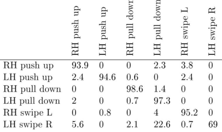
In the second experiment we compared our weighted DTW algorithm against the con-ventional DTW method and a weighted DTW method proposed by [47] using the relaxed gesture database. The confusion matrices for the three algorithms for six chosen gesture

(25)

BH Pull Down BH Push Up LH Pull Down LH Push Up LH Swipe L LH Swipe R LH Wave RH Pull Down RH Push Up RH Swipe L RH Swipe R RH Wave

0 5 10 15 20 25 30 35 Gesture class Discriminant ratio Without pre−processing With pre−processing

Figure 1.8: Discriminant ratios for with and without pre-processed gesture samples using the rotationally distorted gesture database. Note that the discrimant ratios are increased, on average, 42% with the proposed pre-processing method. There are 21 gesture samples in each gesture class. The gesture classes are, namely, Both Hands Pull Down, Both Hands Push Up, Left Hand Pull Down, Left Hand Push Up, Left Hand Swipe Left, Left Hand Swipe Right, Left Hand Wave, Right Hand Pull Down, Right Hand Push Up, Right Hand Swipe Left, Right Hand Swipe Right, Right Hand

Wave, respectively.

Table 1.1: Confusion matrix for the conventional DTW.

RH push up LH push up RH pull do wn LH pull do wn RH swip e L LH swip e R RH push up 93.9 0 0 2.3 3.8 0 LH push up 2.4 94.6 0.6 0 2.4 0 RH pull down 0 0 98.6 1.4 0 0 LH pull down 2 0 0.7 97.3 0 0 RH swipe L 0 0.8 0 4 95.2 0 LH swipe R 5.6 0 2.1 22.6 0.7 69

classes are given in Table 1.1, 1.2, and 1.3. After creating the confusion matrices, we computed the overall recognition accuracies according to the following formula:

A= 100·_P_mTrace(C)

i=1

Pn

j=1C(i, j)

, (1.16)

whereA denotes the accuracy, andC denotes the confusion matrix.

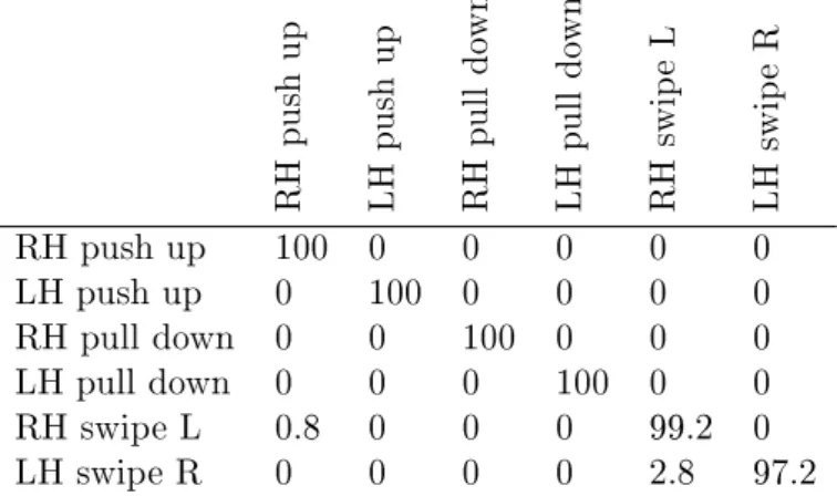
Our proposed method outperforms the weighted DTW method in [47] by a large margin as given in Table 1.4. The reason is that their weights are global weights, i.e., a joint's weight is independent of the gesture class. However, in our proposed method a joint can have a dierent weight depending on the gesture class we are trying to align with. This degree of freedom in computing the associated DTW cost increases the reliability of DTW cost signicantly.

In the third and the last stage, we tested the overall performance of our system using the rotationally distorted and relaxed gesture database. The purpose of this operation

(26)

Table 1.2: Confusion matrix for the weighted DTW in [47]. RH push up LH push up RH pull do wn LH pull do wn RH swip e L LH swip e R RH push up 96.2 1.5 0 0.8 1.5 0 LH push up 3 97 0 0 0 0 RH pull down 0 1.4 98.6 0 0 0 LH pull down 2 0 0 98 0 0 RH swipe L 0 2.4 0 2.4 95.2 0 LH swipe R 7.8 0 0 25.3 0.7 66.2

Table 1.3: Confusion matrix for our proposed weighted DTW.

RH push up LH push up RH pull do wn LH pull do wn RH swip e L LH swip e R RH push up 100 0 0 0 0 0 LH push up 0 100 0 0 0 0 RH pull down 0 0 100 0 0 0 LH pull down 0 0 0 100 0 0 RH swipe L 0.8 0 0 0 99.2 0 LH swipe R 0 0 0 0 2.8 97.2

Table 1.4: Accuracies of the three methods. Note that not only six gesture classes given in Table 1.1, 1.2, and 1.3 are used, but all eight gesture classes are taken into

consideration.

Method Accuracy

Classical DTW 84.41 % State-of-the art 86.56 % Proposed method 97.13 %

is to determine the overall improvement of the pre-processing and the weighting on the recognition performance using a larger database. These experiments clearly demonstrate the performance boost provided by our proposed techniques. The results are given in Table 1.5.

1.6 Conclusion

We have developed a weighted DTW method to boost the discrimination capability of DTW's cost, and shown that the performance increases signicantly. The weights are based on a parametric model that depends on the level of a joint's contribution to a

(27)

Table 1.5: Overall performance comparison using the rotationally distorted and re-laxed gesture database.

Method Accuracy

Traditional DTW 62.41 %

Pre-processing + Traditional DTW 76.26 %

Weighted DTW 84.13 %

Pre-processing + Weighted DTW 96.64%

gesture class. The model parameter is optimized by maximizing a discriminant ratio, which helps to minimize within-class variation and maximize between-class variation. We have also developed a pre-processing method to cope with real life situations, where dierent body shapes and user orientations with respect to the depth sensor may occur.

(28)

Low-Complexity Shape Recognition

Using Random Forest Classiers

with Random Rectangle Features

2.1 Introduction

Shape recognition is an important problem encountered in various applications such as optical character recognition, gesture recognition, medical analysis, and drawing appli-cations [3, 38, 42]. Large number of shape classes, high level of within-class variation, and low level of between-class variation exacerbates the problem. Large number of shape classes necessitates a larger set of training samples to learn which variation in the train-ing dataset contributes to between-class variation. Hence, a good recognition algorithm learns the eect of (combination of) attributes on between-class variation and values attributes accordingly in performing the classication task. High level of within-class variance requires the features to be invariant to some extent to certain transformations and deformations. This requires the features used to be at least partially invariant to these variations. A low level of between-class variation requires the use of features with strong discrimination power or a cascaded application of relatively weaker features (e.g., boosting with Adaboosting) and a larger database to learn such discriminative features. Hence, shape recognition requires a good learning algorithm using either strong features or many weak features. Strong features such as gradient-based statistical features or structural features can be used, but they often have high computational complexity and computing some of these feature can be as dicult as the original classication problem. To achieve fast execution times for real-time applications or low-cost implementations,

(29)

Chapter 2. Shape Recognition 17 weak features are utilized. To increase the accuracy of the classier, cascaded computa-tion of weak features is required. A good example for cascaded learning is the Viola-Jones framework for object detection, which uses a degenerate decision tree [60]. Another ex-ample is bagging of decision trees to increase the accuracy and reduce the variance [55]. In this paper, we use random forest classiers with random rectangle features. Although rectangular features are used in [60] for detection, and random forest classiers are used in many recognition applications with more complex features [12, 17], we propose to use random forest classiers in combination with random rectangle features consisting of a single rectangle. We discuss how partial invariance, and stability is achieved with our random rectangle features as compared to other types of features, and how these two properties are related with cascaded learning characteristics of decision trees in Sections 2 and 3. We further discuss how the parameters of a decision tree and a random forest classier can be optimized to achieve high accuracy, fast execution, and low computa-tional complexity in Sections 4 and 5 by evaluating our proposed method on gesture recognition and optical character recognition. Shape recognition applications in con-sumer products require more ecient use of computation and memory resources without sacricing on the quality. Our proposed method can enable applications in various elds requiring shape recognition with low memory and time budgets, due to its high accuracy, low complexity, and scalability.

2.2 Shape Features for Recognition

Features used in shape recognition can be loosely divided into statistical and structural shape descriptors. Statistical features are direction features utilized within a statistical framework. For example, the histogram of gradients in a locality is used as a descriptor for the orientation. These local gradient histograms can be aggregated via clustering to create global histograms so that not only local but global descriptors are also used as features [33, 35, 37]. Statistical features are invariant to within-class variations such as scaling, rotation, and illumination change [33, 36]. Directions are usually computed after low-pass ltering (e.g., Gaussian ltering), which is performed to remove random varia-tion and improve accuracy. A commonly used type of structural feature is (silhouette) contour descriptors which measure curvature, concavity, convexity, shape-part structure [21]. However, contour features are sensitive to nonlinear variations, structural changes, and articulation [5]. Contour features have lower dimensionality compared to the sta-tistical features, and structural variations that degrade the feature quality can have a signicant overall impact. Skeleton features are another form of structural features which extract the skeleton of the shape. Skeleton features perform better than contour features under structural variations but skeleton stability is often a problem and matching of

(30)

skeleton graphs is still an open research area [6, 11, 24, 51]. Since statistical and struc-tural features are fairly independent descriptors, using statistical and strucstruc-tural features in combination improves the recognition performance [34, 35, 56]. Although statistical and structural features are invariant up to an anity, they are sensitive to image degra-dation. Moreover, statistical and structural features may not always be stable since both statistical and structural features are complex features and require an algorithm working on intensity image data. Oftentimes, a preprocessing (normalization) stage is needed to correct for translation, slant, and rotation. These steps may reduce the robustness due to noise, blur, and illumination changes, etc. On the other hand, random rectangle features are more stable and primitive as compared to statistical and structural features at the expense of being partially invariant.

Important attributes of tree-based rectangle features are (i) cascaded learning, corre-sponding to increasing structure and complexity (ii) partial-invariance, most samples of a given class will more likely give similar responses to similar features as they move down the tree (iii) stability to noise and other randomness since rectangle features do not depend on orientation or other intensity-gradient based features.

Statistical features such as Scale Invariant Feature Transform (SIFT) descriptors are invariant to image translation, scaling, rotation, and partially invariant to local ane distortion and illumination changes [37]. SIFT features uses Dierence of Gaussians (DoG) function applied in scale space to nd key points as feature candidates, which are reduced in the later processing stages. Gradient based descriptors compute quantized gradient histograms on Gaussian smoothed images. Although statistical features are invariant to certain variations, they might not be stable under nonlinear deformations and also require preprocessing stages such as normalization. Hence, statistical features are sensitive to degradation in intensity data such as blur, noise, compression artifacts or distortions in shape due to articulation or human errors, etc. Structural features need contour or skeleton extraction, and detection of structural parts. This task might as well be as complicated as detecting the whole structure, i.e., the shape. For example, recognizing a hole or a line independently may be more dicult than recognizing them jointly as in character "d".

Rectangle features on the other hand are not invariant to translation, scaling, rotation, and projective perturbations in general. However, they are partially invariant and the degree of partial invariance increases with the area of rectangle. If we consider rotation as an example, the area of the shape that resides in a rectangle will vary as the shape is rotated but will vary to a lesser extent if the rectangle is enlarged. At the early stages of a decision tree, larger rectangle features are selected as splitting features, which improves the invariance. This is expected since at lower tree levels class label entropy will

(31)

Chapter 2. Shape Recognition 19 1 2 3 4 5 1 2 3 4 5

Figure 2.1: An example data instance

be larger, therefore same class samples will have high variance compared to same class samples that reside on tree nodes at higher tree levels. Cascaded learning in the form of a tree, will tend to favor larger rectangle features in lower levels. However at higher levels, due to the learning process, entropy of the class labelcwill be smaller and learning will

become a more dicult problem, necessitating more "complex" rectangle features that are smaller or more oriented, i.e., thinner in the horizontal or vertical direction.

2.3 Decision Tree Based Classication

2.3.1 Decision Trees and Random Forests

Decision trees are nonlinear classiers and therefore aim at learning complex boundaries in the feature space using a training data set. The partitions formed by these boundaries are desired to be pure in the sense that each partition contains same class members. Classication of a future sample reduces to nding out which partition the sample lies in, and predicting the class label using the training data in that partition. If the feature space is under-partitioned, the partitions may not be pure enough to accurately predict the class label. On the other hand if the feature space is over-partitioned, partition boundaries might not reect the true boundaries imposed by the data-generation process, and be aected by noise and other random variations in data. Under-partitioning, and over-partitioning corresponds to under-tting and over-tting respectively, which are terms used in classication literature. The under-partitioning leads to a high bias error with low variance in class prediction, and the over-partitioning case leads to a poor generalization performance.

Decision trees ask discriminative questions successively to infer the class of a data sample, and these questions are structured as a tree. Each tree node asks a question about

(32)

F T F T 1 2 3 4 5 1 2 3 4 5 1 2 3 4 5 2 F T 6 7 F T 8 9 5 6 9 8

Figure 2.2: Univariate decision tree

F T 1 2 3 1 2 3 4 5 1 2 3 4 5 2 3

Figure 2.3: Multivariate decision tree

the features of a data sample1_{. The goal in the training phase is to choose the most}

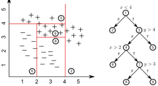
discriminative question to ask at each node. The training data set associated with each tree node is split according to each data sample's answer. A binary decision tree asks YES/NO questions and therefore the training set associated with each node is split into two. A question can be about a single attribute or a combination of attributes of a data sample. The two question types lead to univariate or multivariate decision trees, respectively. The most discriminative question out of a specied set of questions is found as the maximizer of some purity measure such as the negative total entropy in the post-split data sets. A new data sample is classied by sending it down the tree by routing it according to its answers to the questions along its path from the root node to the leaf node. The leaf node predicts the class label using its training samples. Consider the training data samples shown in Figure 2.1. LetI denote a space of 2D points I = (x1, x2). Each I ∈ I has a class label c(I) ∈ C = {+,−}. If single

feature questions are learnt from the training data set, a univariate decision tree of depth four such as the one given in Figure 2.2 can be obtained. However, if questions involve linear combinations of attributes, a multivariate tree that consists of a single node as given in Figure 2.3 can be learnt, and the partitions formed by the decision tree is also shown. As can be seen from the gures, a univariate tree can only split the feature space at a node with a boundary that is orthogonal to the feature axes, resulting in space partitions that are hyperrectangles with sides parallel to the axes. However,

1_{A data sample can be a multi-dimensional vector rather than a scalar value, and each component of}

a data vector is called an attribute of that data sample. A question can involve a single attribute, or a combination of attributes. The rst type of question is called a univariate feature, and the second type of question is called a multivariate feature. In this paper, we use feature and question interchangeably.

(33)

Chapter 2. Shape Recognition 21 more discriminative questions can be asked using a linear combination of attributes, which splits the data space using hyperplanes, resulting in complex polyhedral space partitions. Since univariate questions are more restricted and therefore generally less discriminative than multivariate questions, univariate trees tend to be larger, i.e., more univariate questions are needed to be asked to learn a discrimination boundary between samples of dierent classes.

Although multivariate trees can lead to a better partitioning of the data space, their training is more involved. Selecting attributes to be used in a linear combination for constructing a multivariate question is a dicult problem since the number of linear combinations grow exponentially with the attribute size. Moreover, choosing the com-bination weights is also a problem [14]. For example to classify an image sample, all combinations of attributes (i.e., pixels) grows exponentially with the number of pixels in the image.

Training decision trees by maximizing a purity function at each node is a greedy heuris-tic which causes sensitivity: a small change in the training data set may result in a very dierent decision tree and data space partitioning. This means the classication performance depends on the particular instance of training data set leading to poor gen-eralization performance. To reduce variance, bagging is used to train more than one decision trees on variants of the training set. Predictions of trees can be aggregated by letting each tree vote for a class and making the nal decision in favor of the majority class. Another typical aggregation technique is to create histograms for each leaf node reach in treet to approximate the probability distribution over the class labels Pt(c|I),

and compute the average histogram of all trees.

To improve the bagging performance, random forests reduce correlations between trees by randomization in their training. Randomization is achieved by randomly selecting a set of feature candidates for split decisions in addition to bootstrap techniques to create variants of the training set for each tree. Hence, randomization enforces each tree classier ask dierent questions about the shape which improves the learning-from-data process. Below is a binary decision tree learning algorithm for a random forest

1. Randomly propose K splitting questions Q = {Qi} if size of data set I is large

enough

2. Split the set of examplesI into left and right subsets according to their answer to each question

I_l(Qi) = {I|Qi(I) = YES} (2.1)

(34)

3. Choose the questionQi that maximizes a purity measureP Q∗ = arg max Qi P(Qi) (2.3) P(Qi) = − X s∈{l,r} |Is(Qi)| |I| H(Is(Qi)), (2.4) where negative entropy is used as the purity measure on the class label histograms derived from two split example sets, which are weighted with the cardinality of the two sets.

4. Recurse for left and right example subsets I_l(Q∗) and Ir(Q∗) if the depth in the

tree has not exceeded a pre-dened maximum value.

The above algorithm randomly proposes K questions as candidates for splitting the

examples, exits if a maximum number of depth in the tree is achieved or the pre-split example set does not have enough elements.

2.3.2 Random Forest Classiers For Recognition

Randomized decision trees and forests have been used in multi-class classication prob-lems due to their low complexity and high accuracy[31, 39, 54]. Using random forest classiers, real-time performance can be achieved in dicult computer vision and ma-chine learning problems such as human-pose recognition or gesture recognition [26, 55]. In [55], random forests are used to classify each depth pixel into intermediate body parts that are spatially localized near skeletal joints of interest. Pixel classication into 31 in-termediate body parts transforms the human-pose recognition problem into a multi-class problem that can be eciently solved using random forests in real-time. The features used in split decisions are depth dierences of two pixels in the locality of the current pixel to be classied. The two pixels used in this bivariate feature are obtained by o-setting the current pixelx, and the oset values are normalized using the current pixel's

depth resulting in depth invariant features as given below.

fθ(I,x) =dI(x+ u dI(x) )−dI(x+ v dI(x) ), (2.5)

wheredI(x) is the depth at pixel xin image I. u and v represent the two-dimensional

oset vectors, which are depth-normalized by 1

dI(x). Bivariate features have weak

discrim-inatory power (e.g., if the above pixel is checked and found out to be in the background, the pixel can belong to the head or the two shoulders). Although these features have weak discriminatory power, cascaded use of these features as in the form of a decision tree

(35)

Chapter 2. Shape Recognition 23 reduces the bias of the classier, i.e., a decision tree classier accurately disambiguates the body parts. Moreover, using an ensemble of randomized decision trees (i.e., random forest), the variance of the classier is reduced and the accuracy increases. This system runs at 200 frames per second on consumer hardware thanks to low-complexity depth features and random forest classiers which enable parallel implementation.

Per-pixel random forest classiers are recently used in hand shape recognition on depth image data and tested on American Sign Language (ASL) and hand gesture datasets [26]. High accuracy rates are reported without resorting to the use of color images. Similar to [55] as discussed above, random forest classiers are used on depth images, and the same bivariate depth feature in (2.5) is used for making discriminative split decisions at split nodes.

Recognizing the shape (i.e., human skeleton) in parts (i.e., body joints/parts) necessi-tates per-pixel classication because more than one classes (i.e., body parts) will exist in the same image. Hence, there are segments in the image with dierent class labels. To recognize each segment using more than one pixel, one needs to know where the seg-ments are located, and their boundaries, etc. Therefore, a per-pixel based classication signicantly simplies the algorithm. However, the number of classication problems to be solved increases by the number of pixels. When there is one shape in the image or detection has already been priorly performed to nd the region of interest, shape classication can be performed on the whole image without requiring per-pixel classi-cation. Moreover, a bivariate feature as in (2.5) might not be reliable when the shape structure involves thin structural details oriented in varying directions, which makes the bivariate feature less invariant to structural and "pose" changes, or image degradations. We tailored the technique in [55] for Optical Character Recognition (OCR) by using per-pixel random forest classication together with bivariate features given in (2.5). The error rate was unacceptably high around 40% on the MNIST digit database. However, the same technique applied to Gesture Recognition (GR) on American Sign Langugage (ASL) dataset using only static ASL letters achieved a recognition rate of 85% using only depth data, which is signicantly higher than the state-of-the-art recognition rates (e.g. 75% achieved in [43], see Section 2.5.2 for details). The better performance of per-pixel classication with bivariate features on GR is due to a lesser degree of ne details and structural variations in the hand gestures compared to hand-written digits which can have high degree of structural variation and ne details.

(36)

Figure 2.4: Example Viola-Jones features relative to the detection window. The sum of the pixel intensities in the grey rectangular regions are subtracted from the white

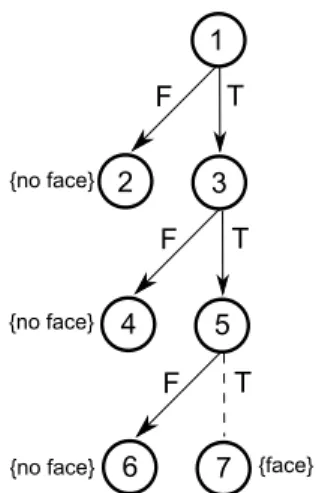
rectangular regions. 1 3 2 4 5 T F 6 7 {no face} {no face}

{no face} {face}

T F

Figure 2.5: Cascaded application of classiers enable focusing on object-like regions.

2.3.3 Viola-Jones Object Detection Framework

To improve the robustness, one can utilize features in the form of a lter that aggregates local information in its support. For example statistical features exploit pyramid lter-ing schemes by uslter-ing steerable lters. Steerable lters can be oriented accordlter-ing to the structural details and can extract more useful information about orientation and shape in a locality [22]. Haar wavelets are examples of such lters. Haar wavelets are used in many applications for recognizing and detecting shapes in the image [4, 63, 67]. First used in face detection, and then used in object detection in general, Viola-Jones features are Haar-like features and compute dierences of intensities in rectangular regions (see Figure 2.4 for some examples features) [60]. With the use of an image representation called the integral image, Viola-Jones features can be computed in constant time inde-pendent of feature scale (i.e., rectangle size). Viola-Jones features consist of adjacent rectangular regions, and the total intensities inside adjacent rectangular regions are ei-ther summed or subtracted to compute the feature value. Adaboosting is used to train a weak classier at each boosting stage. A weak classier is constrained to use a single fea-ture. As a result, classier selection at each boosting stage reduces to a feature selection process. Each classier is trained to have a low false negative rate of approximately 0% and a false positive rate of 40%. These classiers are applied in cascade. Sub-windows

(37)

Chapter 2. Shape Recognition 25 rejected by a classier at any stage of the cascade is not processed further thanks to the very low false negative rate. This method successively discards non-object regions and spends more processing time on regions that resemble the object of interest (see Figure 2.5), thereby achieving real-time execution. The classication structure of the Viola-Jones method is essentially a degenerate decision tree, in which the left nodes are always leaf nodes and are labeled NO. There exists a single leaf node labeled YES and it requires more computation to reach, compared to any other node in the tree.

In object detection the goal is to detect the object inside the image, and the object can be present at any scale and at any spatial location. Hence, the cascaded weak classiers has to process various sub-windows in the image using classiers of varying scale. This means Viola-Jones features of dierent sizes need to be evaluated at dierent spatial locations in the image. On the other hand object recognition assumes object detection has been performed before. Hence, the scale and the location is approximately known. In this sense recognition is a simpler problem compared to detection. But object recognition in general is a multiclass classication problem while object detection is a binary classication problem. Object detection algorithms such as Viola-Jones object detection framework take advantage of this by utilizing (weak) single-feature classiers with low false negatives. The degenerate structure of the decision tree enables early termination for a NO label, which means that regions that are not object-like are reliably labeled early in the process. This is possible because in detection there are two classes and each classier in the cascade is trained for achieving a low false negative rather than both low false negative and low false positive. However, in recognition there are more than two classes and it is dicult to nd a (weak) single-feature classier to recognize a class and create a leaf node for early termination. Hence, a degenerate decision tree would not be a good t for an object recognition task. Cascaded application of more than one weak classiers will be needed to recognize an object leading to more balanced decision trees.

2.4 Random Forest Classiers with Random Rectangle

Fea-tures

We use random forest classiers with random rectangle features for shape recognition. Random forest classiers have lower computational complexity compared to other clas-siers such as support vector machines (SVMs), neural networks, or nearest-neighbor type classiers [55]. Random forest classiers with bivariate features fail to learn the shape structure when there are thin details in the structure because the bivariate (two

(38)

Figure 2.6: Visualization of a decision tree up to the fourth depth level trained on OCR data. The thickness of the edges connecting nodes is proportional to the number of images associated with the receiving node. The average of all training images at a node is displayed. The brightness of the circle below the average image is inversely proportional to the entropy at that node: the higher the entropy the darker the color

of the circle.

pixel) feature may not be stable due to variations in the thin structural parts. For ex-ample using bivariate features for hand-written digit recognition performs poorly with an accuracy rate of 60%. However, rectangle features are more insensitive to in-class variations due to the aggregation of pixels inside a feature's rectangular region. We use a simple feature that consists of a single rectangle, which is even more primitive than the Viola-Jones features. Viola-Jones lters employ simple to complex single-feature classiers starting from two-rectangle features to more complex features involving more rectangles and their various additive or subtractive combinations. This is required be-cause Viola-Jones detection framework uses a degenerate decision tree whose NO-branch is always a leaf node detecting the non-existence of the searched shape. Hence, the false negative rate has to be kept extremely low, which requires asking more and more dif-cult questions (i.e., more complex features as combinations of rectangles). However, a balanced decision tree will continue asking questions both on the YES and the NO branch. Therefore the questions do not need to become dicult: cascaded application of more primitive features will be able to perform successive splits and purify the label distribution.

A rectangle feature is a multivariate feature that uses a combination (summation) of all pixel intensities in a rectangle given by

(39)

Chapter 2. Shape Recognition 27

fr(I) =rTI, (2.6)

where I is a vector of image pixels, and r is a vector of zeros except nonzero elements

of value one corresponding to the pixels inside the rectangle. A rectangle feature can be computed in constant time independent of its size using the integral image [60]. At each split node a set of random features {fr(I)} and threshold candidates {T} are created and out of the corresponding binary questions

{Q= (fr(I)< T) ? YES : NO}, (2.7)

the best question is chosen. An example decision tree up to depth level four trained on OCR data set is shown in Figure 2.6. The red rectangle shows the best split rectangle depicted on the average image, which is the average of all images at that node. The data sets are puried at the higher depth levels and the average images start to resemble one of the ten digits.

2.4.1 Rectangle Feature As A Linear Combination

The best split rectangle feature is a multivariate feature which is a linear combination of attributes (e.g., pixels) with all coecients equal to one. There are two important problems in nding a good linear combination of attributes. The rst is selecting the attributes to be included in the linear combination, and the second is learning their co-ecients. To select the attributes there are two basic approaches: Sequential Forward Selection (SFS) and Sequential Backward Selection (SBS). SFS is a bottom up search method that starts with zero attributes and adds the attribute that causes the biggest increase in the purity measure until a stopping criteria is met. On the other hand, SBS is a top down search method for attribute selection. To learn the coecients of the linear combination, techniques such as Recursive Least Squares (RLS) which minimizes mean-squared error over the training data or CART which explicitly searches for a set of coecients that maximize a purity measure is utilized. Both attribute selection and co-ecient learning applied without any restriction will lead to general multivariate features that are not the sum of pixels in a rectangular area.

To be able to use rectangle features in combination with the integral image, we x all coecients to be one and randomly select attributes by creating a set of random rectangle features rather than a top down or a bottom up search technique. This randomization also improves the accuracy of the random forest classier by reducing the correlation between trees. The best rectangle is chosen as the purity maximizer and then rened

(40)

by perturbing its top-left and bottom-right corners. A typical corner perturbation can be a one pixel horizontal/vertical shift in the two-dimensional space, which results in a set of 25 perturbed rectangle candidates. The split rectangle feature is determined by renement iterations using the corner perturbation technique. Rectangle renement can produce discriminative rectangles, e.g., the split rectangle of the rightmost node at depth level 2 as given in Figure 2.6, which most likely separates 4's and 9's in its data set. Below is the algorithm for training a single tree using random rectangle features.

1. Randomly propose a set of rectangle features{r} and a set of candidate threshold {T} for eachrin{r}

2. Create a question Qi for each randT

3. Split the set of examplesI into left and right subsets according to their answer to each question

I_l(Qi) = {I|Qi(I) = YES} (2.8)

I_r(Qi) = I\Il(Qi) (2.9)

4. Choose the questionQi that maximizes a purity measureP

Q∗ = arg max Qi P(Qi) (2.10) P(Qi) = − X s∈{l,r} |Is(Qi)| |I| H(Is(Qi)), (2.11) 5. Create a new set of questions Q by perturbing left-top and right-bottom corners

ofr∗ ofQ∗

6. Find Q∗∗ inQ by maximizing the purity measure 7. Go to step 5 until an exit criteria holds

8. Recurse for left and right example subsets Il(Q∗∗) andIr(Q∗∗)if the depth in the

tree has not exceeded a pre-dened maximum value.

2.5 Experiments

In this section we describe the experiments performed to evaluate our Random Forest Classier with Random Rectangle Features (RFCwRRF) method. We apply our method to Optical Character Recognition (OCR) and Gesture Recognition (GR), and evaluate