Nonparametric Option Pricing under Shape Restrictions

NBER WORKING PAPER SERIES

NONPARAMETRIC OPTION PRICING UNDER SHAPE RESTRICTIONS

Yacine Ait-Sahalia Jefferson Duarte

Working Paper8944

http://www.nber.org/papers/w8944

NATIONAL BUREAU OF ECONOMIC RESEARCH 1050 Massachusetts Avenue

Cambridge, MA 02138 May 2002

We are grateful to seminar and conference participants, and in particular René Garcia, for their comments and suggestions. The comments of the Editors and three referees were very helpful. This research was conducted during the first author’s tenure as an Alfred P. Sloan Research Fellow. Financial support from the NSF under grants SBR-9996023 and SES-0111140 (Aït-Sahalia) and from the Center for Research in Security Prices at the University of Chicago Graduate School of Business (Duarte) is gratefully acknowledged. The views expressed herein are those of the authors and not necessarily those of the National Bureau of Economic Research.

© 2002 by Yacine Ait-Sahalia and Jefferson Duarte. All rights reserved. Short sections of text, not to exceed two paragraphs, may be quoted without explicit permission provided that full credit, including © notice, is given to the source.

Nonparametric Option Pricing under Shape Restrictions Yacine Ait-Sahalia and Jefferson Duarte

NBER Working Paper No. 8944 May 2002

JEL No. G12, C14

ABSTRACT

Frequently, economic theory places shape restrictions on functional relationships between economic variables. This paper develops a method to constrain the values of the first and second derivatives of nonparametric locally polynomial estimators. We apply this technique to estimate the state price density (SPD), or risk-neutral density, implicit in the market prices of options. The option pricing function must be monotonic and convex. Simulations demonstrate that nonparametric estimates can be quite feasible in the small samples relevant for day-to-day option pricing, once appropriate theory-motivated shape restrictions are imposed. Using S&P500 option prices, we show that unconstrained nonparametric estimators violate the constraints during more than half the trading days in 1999, unlike the constrained estimator we propose.

Yacine Ait-Sahalia Jefferson Duarte

Department of Economics Department of Finance and Business Economics

Princeton University University of Washington

Princeton, NJ 08544-1021 267 MacKenzie Hall

and NBER Box 353200

[email protected] Seattle, WA 98195-3200

1

Introduction

In many settings, economic theory only restricts the direction of the relationship between variables, not the particular functional form of their relationship. Typically, a theory would predict that some economic variableY should increase when some other variableXincreases. Beyond that, the typical economic theory is often not very restrictive about the speciÞc nature of the relationship between Y and X, and if it is, it is often as a result of choosing a particularly tractable model which the theorist understands to be for illustrative purposes only. Sometimes, economic theories manage to put additional restrictions on the shape of the function that links X to Y. For instance, the relationship may be predicted by the theory to be not only monotonic, but also concave. Or it may satisfy some other inequality restrictions on the function and/or its derivatives. Or the function may be homogenous of some degree, or homothetic (i.e., a positive monotonic transformation of the function is homogenous of degree one).

Examples of this nature abound in economics. The cost function of a standard perfectly com-petitive Þrm must be increasing and convex. For such a Þrm, the production function linking its inputs and outputs must be increasing and concave. The utility function of a typical economic agent must be increasing and concave. In fact, the most speciÞc result in this literature, Afriat’s Theorem, states that a utility function can be found to rationalize a set of observations on prices and quantities if and only if it is nonsatiated, continuous, concave and monotonic [see Afriat (1967)]. No speciÞc functional form can be deduced from the axioms of utility theory, yet one would often parametrize the utility function as an exponential function, a power function, a logarithmic function or rely on more complex functional forms.

Of course, stringent parametric assumptions are very useful for a variety of reasons. First, they allow extrapolation beyond the support of the observed data. Many economic policy questions require that hypothetical experiments be performed in the context of the model (what would the effect of a tax cut be on consumption and investment?). Strategic decisions made by Þrm also require extrapolation (how would proÞts be affected if prices were raised further?). Second, it is easy to specify a functional form that will necessarily satisfy the theory-determined restrictions (for example, Y = Ln(X) will always be increasing and concave). Indeed, the common approach in empirical work, for example in microeconometrics, has been to specify parametric functional forms which satisfy the necessary shape restrictions [see e.g., Diewert (1973)]. Third, more general parametric models can be built and tested against nested models that satisfy the restrictions imposed by the theory to see if these restrictions are valid. For instance, if the function is predicted to be increasing and concave and the adopted model isY =Xρ, an estimate of ρ can be readily used to

test the concavity restriction, i.e.,0< ρ <1.Fourth, the theoretical restrictions can be imposed and result in a decrease in the variance of the estimated parameters.

Despite all their advantages, parametric assumptions have their drawbacks. First, any speciÞ -cation error will typically lead to inconsistent estimates. Second, any test of the theory such as that described above is a joint test of the theory and the (essentially arbitrary) parametric model. Changing the parametric speciÞcation of the model will produce different answers. As a result, non-parametric methods are often used in empirical work, at least as a Þrst step in the analysis of the data useful to guide the speciÞcation effort. With nonparametric methods, it becomes possible to examine say, whether Y increases withX, without assuming a particular model for the conditional expectation of Y given X. Unfortunately, nonparametric estimators pay for their robustness to speciÞcation errors in other ways. They converge more slowly than their parametric counterparts, thereby requiring a larger sample size to achieve the same degree of accuracy —often, but not always, a small price to pay for the elimination of misspeciÞcation risk. Moreover, their rate of convergence deteriorates even further when derivatives of the function are estimated. Consequently, in small samples, the estimatedÞrst and second derivatives of the function of interest can often fail to satisfy the restrictions that the theory imposes, simply because of sampling noise.

It is therefore quite natural for the literature to have evolved towards estimates that are non-parametric in nature, yet satisfy whatever theory-motivated properties are appropriate. The main body of literature deals with the use of monotone restrictions to estimate a nonparametric regression [see Barlow et al. (1972), Robertson et al. (1988) and Matzkin (1994) for an excellent survey]. A common model isY =m(X) +ε,where either the expected value or the median ofεgivenX is zero and m(_·) is estimated by minimizing the least squares or least absolute deviations of the residuals, under the constraint that it be monotonous. Brunk (1970) and Hanson and Pledger (1973) proved the consistency of the estimator under different assumptions.

While the rate of convergence of the least squares estimator is available [see Wright (1981)], its asymptotic distribution is not yet known. The estimation of concave regression functions (same context as above except that m(_·) is known to be concave) has also been extensively considered [see e.g., Hildreth (1954) and Hanson and Pledger (1976)] and its distribution is known in the least squares case [see Wang (1993)]. Finally, algorithms that extend Hildreth’s to estimate a regression curve under inequality restrictions have been proposed by Dykstra (1983) and Ruud (1997), again in the constrained least squares context. To the best of our knowledge, the asymptotic distribution of these estimators is unknown.

Rather than attempt to solve the least squares (or least absolute deviations) problem, we propose in this paper a method to impose shape restrictions as a simple modiÞcation of nonparametric

locally polynomial estimators. The standard Nadaraya-Watson kernel regression estimator is a special case of a locally polynomial estimator, corresponding to a “locally constant” speciÞcation, i.e., a polynomial of order zero. By modifying locally polynomial estimators, instead of attempting to devise a new type of constrained nonparametric estimator, we can rely on a well-understood set of tools in the unconstrained regression case [see e.g., Fan and Gijbels (1996)]. Moreover, our estimators are smooth like any other kernel-type regression estimator, unlike for instance the estimator produced by solving the constrained least squares problem. Our constrained nonparametric estimators satisfy, by construction, the restrictions imposed by economic theory. We focus on locally linear estimators and on the case where inequality constraints are imposed on the regression function and itsÞrst two derivatives.

As is often the case, and the estimation of option-implied densities inÞnance is no exception, there are many different ways to smooth a curve —Nadaraya-Watson kernel regression as in Aït-Sahalia and Lo (1998), splines with a penalty for lack of smoothness [e.g., Mammen and Thomas-Agnan (1998)], constrained splines [Bates (2000)],ßexible parametric functional forms [in the context of SPDs, see for example Abadir and Rockinger (1998)], neural networks [see Garcia and Gencay (2000) and Haefke, White and Gottschling (2000)], etc. Bates’s paper in particular considers cubic splines estimated under the same constraints as ours, while Bondarenko (1997) considers the same constrained least squares problem we do.

We focus on a particular method, locally polynomial regression. In our view, locally polynomial estimators present a few advantages, some of which are shared by the other possible choices. First, they are truly nonparametric. Second, they have well-documented good small sample behavior [see e.g., Fan and Gijbels (1996)], especially relative to kernel regression estimators. Third, we are able to implement the method in such a way that the locally polynomial estimator will always produce estimates satisfying the constraints, which is also possible with some of the other methods, but in our case turns out to require no modiÞcation to the estimator, only its application to some transformed data. This said, we do not mean to suggest that local polynomials are necessarily a dominating alternative to everything else nonparametric (otherwise there would not be such a long list of available methods!), but rather our objective is to add to the nonparametric toolkit by showing how this particular method can be amended to reßect shape constraints, especially those that are of interest in derivative pricing. This is achieved in our main theoretical result, Proposition 1, which we hope will be of independent interest beyond our application to the estimation of state-price densities. Our estimator extends the results of Mammen (1991). Mammen introduced a two-step kernel regression that results in monotonic estimates. We extend Mammen’s results in three directions. First, we incorporate restrictions in the Þrst and in the second derivatives, which is empirically

relevant in a large number of economic contexts. Second, we work with locally polynomial estimators (locally linear in our speciÞc context) as opposed to the Nadaraya-Watson kernel regression estimator used by Mammen, which is a locally constant polynomial estimator. Third, we allow for a broader class of kernel functions than just the Gaussian kernel; in particular, the popular uniform and Epanechnikov kernels are admissible.

The remainder of the paper is organized as follows. We start in Section 2 by describing the main example that motivates this paper, the kernel estimation of the state-price density implicit in the market prices of traded options. In Section 3 we introduce our estimator and compare it to the unconstrained Nadaraya-Watson and locally linear nonparametric estimators. We show in particular that our estimator will satisfy the constraints imposed in sample and not just asymptotically. The results of a Monte-Carlo analysis of these three estimators are presented in Section 4. In Section 5, we apply our methodology to option pricing. Section 6 concludes. Technical proofs and results are in the Appendix.

2

Monotonicity and Convexity of Option Pricing Functions

The motivation for our empirical work is the theory-imposed restriction that the price of a call option must be a decreasing and convex function of the option’s strike price. Assuming that markets are dynamically complete, the absence of arbitrage opportunities implies the pricing operator is linear. Continuity and linearity of the pricing operator implies by the Riesz representation theorem the existence of a state-price density (SPD), which we denote byp∗(ST|St, τ , rt,τ, δt,τ).1 The call pricing function at timet is then given by:

C(St, X, τ , rt,τ, δt,τ) =e−rt,ττ Z +∞

0

max(S_{T −}X,0)p∗(S_T|St, τ , rt,τ, δt,τ)dST (2.1)

1

The existence and characterization of an SPD can be obtained either in preference-based equilibrium models, e.g., Lucas (1978), Rubinstein (1976), or in the arbitrage-based models by Black and Scholes (1973) and Merton (1973). In the equilibrium framework, the SPD can be expressed in terms of astochastic discount factor orpricing kernel such that asset prices are martingales under the actual distribution of aggregate consumption after multiplication by the stochastic discount factor.

Among the no-arbitrage models, the SPD is often called therisk-neutral densitybased on the analysis of Cox and Ross (1976) who observed that the Black-Scholes formula can be obtained by assuming that all investors are risk neutral and, consequently, all assets in such a world must yield an expected return equal to the risk-free rate of interest. The SPD also uniquely characterizes theequivalent martingale measure under which all asset prices discounted at the risk-free rate of interest are martingales [see Harrison and Kreps (1979)], and thestate-price deßator [see Duffie (1996)].

whereStis the underlying asset price at datet,Xthe strike price,τ the time-to-expiration,T =t+τ the expiration date, rt,τ the risk free interest rate for that maturity, and δt,τ the corresponding dividend yield of the asset. In what follows, we will leave the conditioning information implicit, and writep∗(ST) for p∗(ST|St, τ , rt,τ, δt,τ).

In order to rule out arbitrage opportunities,C must be a decreasing function of X and theÞrst derivative of C with respect toX must be greater than ₋e−rt,ττ_{. This follows from (2.1) since}

∂C(St, X, τ , rt,τ, δt,τ) ∂X =−e −rt,ττ Z +∞ X p∗(ST)dST (2.2) thus from the positivity of the density and its integrability to one

−e−rt,ττ

≤ ∂C(St, X, τ , r_∂X t,τ, δt,τ) ≤0 (2.3) By differentiating the call price function twice with respect to the strike price, one obtains, as in Breeden and Litzenberger (1978) and Banz and Miller (1978):

∂2C(St, X, τ , rt,τ, δt,τ)

∂X2 =e−

rt,ττ_p∗_(X)

≥0 (2.4)

i.e., ∂2_C(·)/∂X2 _{is proportional to a probability density function and hence must be positive. Any} local non-convexity of the call pricing function implies negative state prices, which constitute a violation of the no arbitrage principle.

Thus theÞrst two derivatives of the “cross-sectional” option pricing function X _7−→Ct,τ(X) ≡ C(St, X, τ , rt,τ, δt,τ) for given (St, X, τ , rt,τ, δt,τ),i.e., at each point in time t and for each maturity τ ,must satisfy the set of inequality constraints

   −e−rt,ττ _≤C0 t,τ(X)≤0 C_t,τ00 (X)_≥0. (2.5) The theory also imposes no arbitrage bounds for the call option pricing function itself:

max³0, Ste−δt,ττ−Xe−rt,ττ ´

≤Ct,τ(X)≤Ste−δt,ττ. (2.6) Note Þrst that it follows from (2.1) and (2.4) that C_t,τ00 (X) _≥ 0 implies Ct,τ(X) ≥ 0. Secondly, if the price Ft,τ at t of a forward contract for delivery of the underlying asset at date T = t+τ is observable, then by no arbitrage

Ft,τ = e−rt,ττ Z +∞

0

STp∗(ST)dST

In this case, it follows from the fact that max(ST −X,0) ≤ ST and from (2.1) and (2.7) that Ct,τ(X)≤Ste−δt,ττ.It also follow these equations and the fact that p∗ is a density that Ct,τ(X) ≥ Stexp(−δt,ττ)−Xexp(−rt,ττ).Indeed,

ert,ττ n Ct,τ(X)−Ste−δt,ττ+Ke−rt,ττ o = Z +∞ X (ST −X)p∗(ST)dST − Z +∞ 0 STp∗(ST)dST +X = Z X 0 (X₋ST)p∗(ST)dST ≥ 0.

These restrictions can be expressed as restrictions onC_t,τ00 (X),by writing them in the form Z +∞ 0 C_t,τ00 (X)dX = e−rt,ττ _(2.8) Z +∞ 0 XC_t,τ00 (X)dX = Ft,τ. (2.9)

Therefore, the constraints imposed by the theory can all be summarized in terms of the functions C_t,τ0 (X) and C_t,τ00 (X), and our primary objective in this paper will be to construct nonparametric estimators of the functions X _7−→C0

t,τ(X) and Ct,τ00 (X) that satisfy the constraints (2.5), (2.8) and (2.9).

Aït-Sahalia and Lo (1998) proposed to estimate the SPD nonparametrically by using market prices to estimate an option-pricing formulaCˆ(_·)nonparametrically, then differentiate this estimator twice with respect toXto obtain∂2Cˆ(_·)/∂X2. Under suitable regularity conditions, the convergence (in probability) ofCˆ(_·)to the true option-pricing formulaC(_·)implies that∂2_Cˆ_(·)/∂X2 _{will converge} to∂2C(_·)/∂X2. Consequently, to arrive at the SPD from (2.4) it is sufficient to estimate the second derivative of the call price function in relation to the strike price. Without any restrictions on the full nonparametric regression of call prices of stock value, strike, time-to-maturity, interest rate and dividend yield, the estimates are too variable to be useful in practice. Therefore Aït-Sahalia and Lo (1998) reduced the dimensionality of the regression function by using a semiparametric speciÞcation. Suppose that the call pricing function is given by the parametric Black-Scholes formula

C_BS(Ft,τ, X, τ , rt,τ;σ) =e−rt,ττ{Ft,τΦ(d1)−XΦ(d2)} (2.10) whereFt,τ =Stexp((rt,τ−δt,τ)τ)is the forward price for delivery of the underlying asset at date T and d1≡ ln(Ft,τ/X) + (σ2/2)τ σ√τ , d2≡d1−σ √ τ (2.11)

option’s moneynessMt,τ ≡X/Ft,τ and time-to-maturityτ:

C(St, X, τ , rt,τ, δt,τ) =CBS(Ft,τ, X, τ , rt,τ;σ(X/Ft,τ, τ)). (2.12)

In this semiparametric model, they only need to compute the lower-dimensional kernel regression of implied volatilities on moneyness Ft,τ, X and τ to estimate σˆ(·). The rest of the call pricing functionC(St, X, τ , rt,τ, δt,τ)is parametric, thereby substantially reducing the sample size of options required to achieve the same degree of accuracy as the full nonparametric estimator. This approach nevertheless has its own drawbacks. First, it is not fully nonparametric. Second, it still requires a fairly large sample size to be effective. In a typical cross-section of options at one point in time, one often observes the prices of20to50options with different strike prices (for a given maturity). This limitation of the traded strikes is a consequence of a deliberate strategy on the part of the options exchanges to insure that the market for each one of them remains sufficiently liquid. Enlarging the sample by gathering data from different dates is useful for data description purposes but opens the door to potential nonstationarity and regime shift issues. Moreover, the inputs of interest, such as the underlying assets price, its volatility or the interest rate, can be volatile enough to preclude aggregating data from different days.

Finally, it is possible for the implied volatility smile function σ(X/Ft,τ, τ) to have sufficiently large derivatives with respect to the option’s moneynessMt,τ for the resulting semiparametric SPD to violate the nonnegativity constraint, especially for long-term options. That is, differentiating (2.12) yields    ∂C ∂X = ∂CBS ∂X + 1 F ∂σ ∂M ∂CBS ∂σ ∂2C ∂X2 = ∂2_C BS ∂X2 +_F2_∂M∂σ ∂2_C BS ∂X∂σ + 1 F2 ¡_∂σ ∂M ¢2_∂2_C BS ∂σ2 +_F12 ∂ 2_σ ∂M2 ∂CBS ∂σ

and the right hand sides of these expressions need not satisfy the respective constraints that their left hand sides should satisfy.

Non- and semiparametric estimators of the call pricing function will satisfy the restrictions in theÞrst and second derivatives only when the sample is large enough, and the true function veriÞes them. This follows simply from the pointwise convergence of nonparametric regression estimators and their derivatives. As in all the other examples from economic theory discussed above, nonpara-metric estimates may violate the theory-imposed convexity restriction, but paranonpara-metric estimates can misspecify interesting properties of the SPD (such as its skewness and kurtosis patterns) because they are overly rigid.

where economic theory places no restrictions on the function other than the inequality restrictions (2.5). Because of the potential risk involved in misspecifying the SPD, it is desirable not to impose tight parametric restrictions on the density. And the constraints imposed by the theory provide no guidance whatsoever in terms of specifying a parametric model for the SPD. In fact, as long as the candidate parametric SPD is a proper density function, no matter how it is speciÞed parametrically, the constraints will be satisÞed. Moreover, only when sufficiently strong assumptions are made on the underlying asset-price dynamics can the SPD be obtained in closed form. For example, if asset prices follow geometric Brownian motion and the riskfree rate is constant, the SPD is log-normal– this is the Black-Scholes/Merton case. For more complex stochastic processes, the SPD cannot be computed in closed-form and must be approximated by numerically intensive methods. So this is a typical situation where we need a nonparametric estimator that can be constrained to satisfy given shape restrictions.

3

Constrained Nonparametric Estimation

To obtain a nonparametric estimator satisfying the required shape properties, we use a combination of constrained least squares regression and smoothing.

3.1

Constrained Least Squares Regression

The problem of constrained least squares regression consists in Þnding the closest values mi, in the sense of least squares, to a set of n observations y1, y2, ..., yn satisfying a set of constraints. Bondarenko (1997) also uses constrained least squares in the same context as we do. The constraints involvenobservations on an explanatory variable,x1, x2, ..., xn.In our case,yi is the price of the call option with strike xi. Without loss of generality assume that the observations on the explanatory variable have been ordered, i.e.,xi≥xj fori > j, i, j∈{1,2, ..., n}.

The constrained least squares regression consists in Þnding the vector m that solves, for the observation vectory: min m∈Rn n X i=1 (mi−yi)2 = min m∈Rnkm−yk 2 (3.1) subject to the slope and convexity constraints:

   −e−rt,ττ _≤ mi+1−mi xi+1−xi ≤0 for all i= 1, ..., n−1 mi+2−mi+1 xi+2−xi+1 ≥ mi+1−mi xi+1−xi for alli= 1, ..., n−2 (3.2)

If we were only imposing monotonicity of the pricing function, then this would reduce to the classical isotonic regression [see e.g., Barlow et al. (1972)]. We can eliminate some constraints that are redundant. The convexity constraints insure that the slopesMi+1,i ≡(mi+1 −mi)/(xi+1−xi) are nondecreasing. Therefore the inequality constraints on the interior slopes (i= 2, ..., n₋2) are redundant and only the boundary slope constraints (lower bound for i = 1 and upper bound for i=n₋1) matter. Therefore the constraints (3.2) can be rewritten as

   m1−m2 x1−x2 ≥ −e −rt,ττ _{and m} n−1−mn≥0 mi+2−mi+1 xi+2−xi+1 ≥ mi+1−mi xi+1−xi for all i= 1,2, ..., n−2 (3.3) This reduces the total number of constraints from2n₋3ton,which has computational implications when nis moderately large.

Note that the price constraint corresponding to (2.5) can be imposed as

max³0, Ste−δt,ττ−xie−rt,ττ ´

≤mi ≤Ste−δt,ττ for all i= 1, ..., n.

In light of the monotonicity constraints already present, these nconstraints can be reduced to Ste−δt,ττ−x1e−rt,ττ ≤m1 ≤Ste−δt,ττ and mn≥0. (3.4) In any event, the three additional constraints (3.4) need not be implemented at this stage. As we discuss later in Section 3.6, we will obtain an estimator of the pricing functionCt,τ directly from the SPD estimator, i.e., fromC_t,τ00 up to discounting, and provided the SPD estimator satisÞes constraints (2.8)-(2.9) —which we will insure— our price function estimator will satisfy the constraints (2.5).

When the strike prices are equally spaced,xi+1−xi =∆x for alli, which is the case in most if not all options markets, the second constraint in (3.3) becomes

mi+2+mi−2mi+1≥0 (3.5)

which says that the butterßy portfolio constructed by buying a call struck atxi+2,one struck atxi and selling two calls struck atxi+1 must have a nonnegative price.

When solving the constrained minimization problem, we are effectively “cleaning” the datayi in a non-arbitrary manner. Of course, we mean to apply this step after obvious data recording errors (such as a price recorded as 0, etc.) have been corrected. Solving this problem can be contrasted to the commonly used practice of simply deleting from the sample the recalcitrant observations — those that fail to satisfy the arbitrage restrictions— under the rationale that they must be the result of unacceptable measurement errors. Besides being questionable as a general practice, deleting

observations can be quite damaging when the sample is tiny to start with.

Naturally, in cases where the constraints are satisÞed by the original option prices, the solution is simply mi =yi for all i= 1,2, ..., n.But how often is this not the case empirically? Based on the full year 1999, violations of the constraints (3.3) occurred 24% of the time in the raw high frequency S&P 500 index option data from the Chicago Board Options Exchange (lower frequency observations have lower violation occurrences). Hentschel (2001) provides more evidence regarding how noisy the raw option data are.

Finally, the least squares criterion function (3.1) can be weighted as in

min m∈Rn n X i=1 (mi−yi)2ωi (3.6)

to reßect the relative liquidity of different options. In this framework, more actively traded options would receive a higher weightωi than those less actively traded. Readily available data can be used for that purpose. In transaction-level data, the actual weights can be determined on the basis of the size and time of the most recent transaction and the bid-ask spread. In closing prices, the open interest and the bid-ask spread can be used to proxy for liquidity.

Solving the constrained least squares problem has a long history. Von Neumann (1950) originally proposed to solve it using alternative projections. While this insight remains at the heart of the more modern algorithms, Von Neumann’s approach was limited in the possible set of constraints. Hildreth (1954), then Dykstra (1983) progressively extended the set of possible constraints to convex cones (a cone is such that if the solution vectormbelongs to it thenλmalso belongs to it for any constantλ). This would suit our purposes, except that the lower bound constraint on the slopes in equation (3.3) make that constraint affine (a convex set) instead of linear (a convex cone). We show in Appendix A that we canÞrst transform it to one with conic constraints, to which we can then apply Dykstra’s algorithm. We also describe Dykstra’s algorithm, applied to the transformed problem, in Appendix A.

3.2

Locally Polynomial Kernel Smoothing

We now have the transformed data mi. The transformed data (notyi) then serve as inputs to the next and last step in our procedure. This step involves smoothing the transformed datami and we wish to do so in a way that preserves the constraints that were enforced in the previous step.

Let us now turn to a brief description of locally polynomial regression, which allows us also to introduce some notation. Suppose that the regression function m(z) _≡ E[Y_|Z =z] is to be approximated locally forzin a neighborhood of a given state valuexby Taylor’s formula up to order

p m(z)_≈ p X k=0 β_k(x)_×(z₋x)k (3.7)

withβ_k(x)_≡m(k)(x)/k!. This representation of the functionmsuggests modeling m(z) aroundx by a polynomial inz, and to use the regression ofm(z)on powers of(z₋x)to estimate the coefficients β_k. To insure that the estimated coefficients reßect the local nature of the representation, we should intuitively use a weighted regression putting more weights on points close to x. A natural way to achieve this is to introduce a kernel functionK(.), a bandwidthhand to use as weightsKh(xi−x)≡ K((xi−x)/h)/h. This leads to the estimates of the coefficients βbk(x) as the minimizers of

n X i=1 ( mi− p X k=0 β_k,p(x)_×(xi−x)k )2 Kh(xi−x) (3.8)

which is, at each Þxed point x, a generalized least squares regression of the m0_is on powers of the

(xi−x)0swith diagonal weight matrix formed by the weightsKh(xi−x). This regression is “local” in the sense that the regression coefficients in equation are only valid in a neighborhood of each point x.

The estimates of the regression function (and its successive derivatives) are then given by

ˆ

m(k)(x) _≡ mˆk,p(x) = k!βbk,p(x). (3.9) In particular, mˆ (x) _≡ bβ_0,p(x) is the coefficient of the constant term in the polynomial regression of degreep. In this framework, the classical Nadaraya-Watson kernel regression corresponds to the special case of a “locally constant” estimator where the polynomial is reduced to a constant term, i.e., p= 0. Indeed, ˆ m0,0(x) = n P i=1 Kh(xi−x)mi n P i=1 Kh(xi−x) = n P i=1 kimi n P i=1 ki (3.10)

where the heteroskedastic weights are ki = Kh(xi−x), is the generalized least squares (GLS) regression coefficient of themi’s on a constant.

More generally, the GLS estimatorβˆ_p = (ˆβ_0,p,βˆ_1,p, . . . ,βˆ_p,p)0 can be written as ˆ β_p=         Sn,0 Sn,1 · · · Sn,p Sn,1 Sn,2 · · · Sn,p+1 .. . ... ... ... Sn,p Sn,p+1 · · · Sn,2p         −1        Tn,0 Tn,1 .. . Tn,p         (3.11) where Sn,j = Xn i=1(xi−x) j_k i and Tn,j = Xn i=1(xi−x) j_m iki. (3.12) The sumsSn,j andTn,j depend onx, but we leave that dependence implicit to keep the notation simple. In particular if p= 0(Nadaraya-Watson case),mˆ_0,0(x) =Tn,0/Sn,1 , while if p= 1(locally linear regression), we have

ˆ

m0,1(x) = ˆβ0,1=

Sn,2Tn,0−Sn,1Tn,1 Sn,2Sn,0−Sn,12

(3.13) which can be rewritten in the form

ˆ m0,1(x) = Pn i=1wimi Pn i=1wi

where the regression weights are wi ≡ ki{Sn,2−(xi−x)Sn,1} compared to ki in the Nadaraya-Watson case of equation (3.10). Therefore the locally linear estimator assigns weights that are asymmetric, whereas the Nadaraya-Watson weights are always symmetric. This turns out to be a critical improvement especially when x is near the boundaries of the support, i.e., in the tails of the distribution. There, the locally polynomial regression assign weights that adjust for the relative scarcity of the data, unlike those assigned by the locally constant Nadaraya-Watson estimator.

3.3

Estimation of Derivatives

To estimate the derivative of order kof the regression functionm, we can simply setp=k+ 1and use the estimatormˆk,p obtained from equation (3.9).For instance, a locally linear regression serves to estimate the regression function mˆ0,1, a locally quadratic regression for the Þrst derivative mˆ1,2 and a locally cubic regression for the second derivativemˆ2,3. This is generally the optimal choice on the basis of asymptotics (see (3.17) below). But alternatives are available, and they may outperform the asymptotic optimum in small samples. The Nadaraya-Watson estimator in equation (3.10) can easily be differentiated to yield an estimator of the partial derivative ofm(x) with respect tox.

ˆ m0_0,0(x) = ( Pn i=1ki0mi) (Pn_i=1ki) − (Pn_i=1kimi)(Pni=1k 0 i) (Pn_i=1ki)2 (3.14) where k_i0 = (1/h)K0((x₋xi)/h). Further differentiation of (3.10) will produce an estimator of the second derivativem00

0,0(x).

We can also consider the estimators mˆ0,1 for the regression function,mˆ1,1 for itsÞrst derivative and mˆ0_1,1 for the second derivative. In this case,

ˆ m1,1(x) = ˆβ1,1 = Sn,0Tn,1−Sn,1Tn,0 Sn,2Sn,0−Sn,12 = Pn−1 i=1 Pn j=i+1(xi−xj)(mi−mj)kikj Pn−1 i=1 Pn j=i+1(xi−xj)2kikj (3.15) from whichmˆ0

1,1 follows. Our shape-constrained estimator is based on applying the latter estimators to the transformed datami rather than the original datayi.We show below that this insures that the desired shape restrictions are satisÞed in sample, not just asymptotically. For comparison purposes, we also consider the unconstrained estimatorsmˆk,2fork= 0,1,2,corresponding to a locally quadratic regression, andmˆk,3 for k= 0,1,2,corresponding to a locally cubic regression.

3.4

A Word on Asymptotics

Under standard regularity conditions, bothm_b(x)and its derivatives converge pointwise to their true values, as the sample sizengoes to inÞnity. Assume that the conditional expectationm(x) admitsq continuous derivatives. The best achievable asymptotic rate of convergence of the estimatormˆ(k)_(x) of thek-th derivative of m(x) —in the integrated mean-squared error sense— is given by:

n(q−k)/(1+2q) (3.16)

This is actually the best rate of convergence that can be achieved by any nonparametric estimator [see Stone (1982)]. The fact that the rate of convergence in equation (3.16) slows down as the order kof the derivative to be estimated increases is often referred to as the curse of differentiation. This rate is achieved for instance by the Nadaraya-Watson kernel regression when the bandwidth satisÞes h = O(n1/(1+2q)). In the case of locally polynomial estimators, the optimal choice of polynomial order pon the basis of asymptotics is given by

p=k+ 1 (3.17)

(see Fan and Gijbels (1996, Section 3.3)).

work, however, the slow rate of convergence of the derivative estimators can be a major hindrance. In our empirical application, the object of interest is the second derivative of the call option pricing function, Ct,τ(·), with respect to the options strike price, X, when the sample size is of the order of 20 to 50 observations. The asymptotic guidance given by (3.17) would lead to locally quadratic estimators to estimate C_t,τ0 and locally cubic ones for C_t,τ00 . We compare below these unconstrained (but asymptotically optimal) estimators to our constrained locally linear procedure. Monte Carlo simulations immediately reveal that the asymptotics are a poor guide in terms of predicting the behavior of the estimators for such small sample sizes and hence as a guide to selecting them. More-over, as we illustrate in Figures 1 to 3, the constraints are quite often violated by the unconstrained nonparametric estimators with these sample sizes. In addition, we would ideally like an increase in the sample size n to correspond to an increase in the number of strike prices for which prices are observed rather than additional prices obtained at a different point of time for the same strikes. The latter could potentially introduce nonstationarity, with prices at a different instant drawn from a different state-price density. But then collecting data for additional strikes requires going to the over-the-counter market where quotes can be obtained beyond and between the Exchange’s limited traded strikes. Liquidity issues can be substantial. For all these reasons, we are interested in con-structing estimators that will be nonparametric in nature, yet will not require large sample sizes to satisfy the constraints — we want them to satisfy the desired constraintsin sample, rather than just asymptotically.

3.5

Bandwidth Selection

A bandwidth of h= 0results in interpolating each data point (the most complex model), whereas a bandwidth of inÞnity results in a single global polynomial Þt of degree p throughout the sample (the simplest model). How to choose the bandwidth is therefore equivalent to choosing the model’s complexity. Hence it is highly desirable to rely on automatic procedures that remove any potential arbitrariness in the bandwidth’s choice. By minimizing the conditional mean-squared error atx

n E h ˆ m(k)(x)_|x i −m(k)(x) o2 +V ar h ˆ m(k)(x)_|x i (3.18) the optimallocal (i.e., variable withx) bandwidth is (see e.g., Fan and Gijbels (1996)):

hlocal(x) =Ck,p " v(x) © m(p+1)_(x)ª2_π(x)× 1 n #1/(2p+3) (3.19) whereπ(x) is the marginal density of the regressors andv(x)their variance.

weighted mean integrated squared error with weight functionω(x) Z ½n E h ˆ m(k)(x)_|x i −m(k)(x) o2 +V ar h ˆ m(k)(x)_|x i¾ ω(x)dx (3.20) produces the optimal bandwidth

hglobal=Ck,p " R v(x)ω(x)/π(x)dx R © m(p+1)_(x)ª2_ω(x)dx× 1 n #1/(2p+3) (3.21) The constantsCk,p depends upon the choice of the kernel. For example, for the Gaussian kernel K(u) = exp(₋u2/2)/√2π, the relevant constants are C0,1 = 0.776, C0,3 = 1.161, C1,2 = 0.884and C2,3 = 1.006. The bandwidth expressions involve unknown quantities: π(x), v(x) and m(p+1)(x), which all need to be estimated prior to the calculation of the optimal bandwidth. A simple way to do so is byÞtting a polynomial of orderp+ 3globally tom(x), i.e.,m(x) =Pp+3_k=0αkxkestimate the parameters αk by ordinary least squares,v by the sum of squares of residuals (so that the estimator is independent of x), and m(p+1)_{(x) as the second order polynomial obtained by differentiation of} the polynomial Þt of orderp+ 3 of m(x), i.e.,

m(p+1)(x) =Xp+3

k=p+1αkk(k−1)...(k−p+ 1)x

k−(p+1) _(3.22) For the global optimal bandwidth, a typical choice of weighting function would beω(x) =ω0(x)f(x) whereω0(x)is a Þxed function (for instance ω0(x) is 1 for allx between the mean of the xi’s minus 1.5 times the standard deviation of thexi’s and the mean plus 1.5 times the standard deviation, and 0 forx outside this interval). In this case, Rω0(x)dx= 3

p

V ar(X), estimated by replacingV ar(X)

by the sample moment. The estimated optimal global bandwidth is then

ˆ hglobal=Ck,p " ssr_×Rω0(x)dx Pn i=1 © m(p+1)_(X i) ª2 ω0(Xi) ×_n1 #1/(2p+3) (3.23) wheressr is the sum of squares of residuals from the regression (3.22).

3.6

The Result: Estimation Under Inequality Constraints

We now show that the two-step procedure we proposed, namely constrained least square regression of the data followed by a locally linear estimation using the transformed data, results in an estimator satisfying the constraints. The following proposition states our result. The shape-constrained esti-mator we described will always satisfy the constraints for every sample size, not just asymptotically: Proposition 1 Consider a set of n observations on the dependent variables, y1, y2, ..., yn and the

i > j, i, j _{∈ {}1,2, ..., n_}. Assume that the transformed datami result from applying the constrained

least squares algorithm to the original data yi. Then the locally linear estimator obtained from

the transformed data and a log-concave kernel function satisÞes the required constraints in sample:

−e−rt,ττ _≤mˆ(1)_{(x)≤0,and mˆ}(2)_(x)≥0.

Proof: See Appendix B.

The last two constraints (2.8)-(2.9) on the functionmˆ(2)(x)are easily satisÞed. Restriction (2.8) is a scaling constraint: replacingmˆ(2)(x)byexp(₋rt,ττ) ˆm(2)(x)/

R+∞

0 mˆ

(2)_{(z)dzproduces the desired} result. Restriction (2.9) amounts to aÞxed translation of the estimated density to achieve the desired expected valueFt,τ :replace mˆ(2)(x) by the shifted functionmˆ(2)(x−z) with theÞxed shift amount z determined by setting the expected value of the resulting function to the desired levelFt,τ. As we show in Section 4 below, these two adjustments have very little effect on the estimator in practice.

We then deÞne the estimator mˆ(0)(x) of the call pricing function from the SPD estimator by

ˆ

m(0)(x)_≡

Z +∞

0

max(z₋x,0) ˆm(2)(z)dz (3.24) (with an obvious generalization if we wish to price another European-style payoff: just replace

max(z₋x,0)by that contingent claim’s payofffunction). The estimatormˆ(0)_{(x) will automatically} satisfy the no-arbitrage bounds (2.6) satisÞed by the call pricing function. In effect, having a proper SPD estimator in the form of exp(₋rt,ττ) ˆm(2)(x) will automatically result in the price function satisfying the arbitrage bounds appropriate for its payoff structure (in particular, (2.6) for a call option). In the case of American-style payoffs, this would include adding to the right hand side of (3.24) a supremum over the dates over which exercise may occur.

Finally, while we are motivated by the problem of constraining our locally polynomial estimator to have bounded Þrst derivatives and to be convex, it should be noted from the proof that the proposition in fact applies to more general inequalities on the Þrst two derivatives of the function,2 not just the speciÞc ones of interest in the context of estimating SPDs. The assumption that the kernel density function is log-concave is not much of a restriction since that class of kernel functions contains among others the Gaussian, uniform, Epanechnikov and Laplacian kernels, i.e., most of the kernels used in practice.

2_{If the inequalities are modiÞed, then the constraints in the constrained least squares need of course to be modiÞed}

4

Monte Carlo Analysis

4.1

Comparison with Unconstrained Nonparametric Estimators

We perform a Monte-Carlo analysis to determine the performance of the shape-constrained non-parametric SPD estimator and compare it to the standard unconstrained Nadaraya-Watson and locally linear nonparametric estimators. The natural terrain to apply these tools involve S&P 500 index options, so we calibrate our Monte Carlo simulation experiments to match the basic features of this market. We assume that the true price function is the Black-Scholes/Merton model with a implied volatility smile curve. Naturally, the advantage of our nonparametric approach lies in its robustness. If the options were priced by another formula, the nonparametric approach should be able to approximate it as well since, by deÞnition, it does not rely on any parametric speciÞcation for the underlying asset’s price process. Therefore, similar Monte Carlo simulation experiments can be performed for alternative option-pricing models. However, we choose to perform the simulation experiments under an implied volatility smile model designed to be realistic for a typical trading day in 1999. The smile curve used as the data generating process for the simulations was calibrated based on the smile observed on May 13, 1999 on options on the S&P 500 traded at the Chicago Board Options Exchange (CBOE) with expiration in July. The assumed smile is a linear function of the strike with volatility equal to 40% at the strike price 1000 and 20% at the strike price 1700. We set the spot price St at 1365. The short term interest rate and the dividend yield are set at rt,τ = 4.5% and δt,τ = 2.5%, respectively. We consider both the 30 and 60 maturities and plot the results for the 30-day options. The 60-day results are qualitatively similar.

We assume that we observe n = 25 option prices with strike prices equally spaced between 1000 and 1700, as would be the case with actual data. To create simulated option prices, we add uniformly distributed noise to the theoretical option prices. There are two possible rationalizations for the amount of noise to introduce around the assumed “true” option prices in order to carry out simulations. First, the noise can model the bid-ask spread and the different liquidity of different options. Second, we can assume that there is a true set of option prices at one point in time and introduce noise to capture the time series variations of the option prices in a short window of time around that date, after accounting for the variation of the underlying asset price in the same window. In theÞrst approach, the assumed bid-ask spread, calibrated to the market data, is set to 5% of the option’s ask price, with aßoor at 50 cents and a cap at 2 dollars. The noise distribution around the theoretical price is then uniform between 0 and half of the bid-ask spread value. We also account for the different liquidity of options with different degrees of moneyness (most of the liquidity is near the money). SpeciÞcally, recall that the option’s moneyness isMt,τ ≡X/Ft,τ (strike divided by the

forward value of the S&P 500). The noise distribution around the theoretical price is then uniform between 0 and half of the bid-ask spread value times a liquidity factor given by1 + (2/0.2)_|Mt,τ−1|. This makes the liquidity factor1 at the money (Mt,τ = 1) and 2 at Mt,τ = 0.8 or 1.2, and proxies for the observed differences in liquidity of these options.

In the second approach, we calibrate the noise to the typical intraday variation of S&P500 option prices, using their range to calibrate the uniform distribution of the noise term. In percentage terms, the range of values reached stretches from 3% of the option value for deep in the money options to 18% for deep out of the money options. In terms of the performance of the estimators, both models for the noise term produce qualitatively similar results with the provision that the lower the amount of noise, the lower the RMSE performance advantage of the constrained estimator over the unconstrained locally linear estimator (since fewer simulated data samples violate the constraints). This being said, one may argue that any violation of arbitrage constraints (such as those produced by the unconstrained estimator) is potentially much more damaging than its mere RMSE effect (it could for instance induce trading on a false perceived arbitrage) and should be penalized accordingly when assessing an estimator’s performance. Also, other things equal, more noise tends to increase the advantage of the constrained estimator. Nevertheless, the amount of noise we speciÞed above is not unrealistically high. It is in fact, if anything, too conservative: see the empirical evidence in Hentschel (2001).

For estimation, we use a Gaussian kernel. We select a range of bandwidths including those given in Section 3.5 and repeat the estimation steps for each bandwidth value. Then for each function to be estimated, we selected the optimal bandwidth on the basis of minimizing the small sample

weighted mean integrated squared error given in equation (3.20). We discuss this further below. The Monte-Carlo averages and conÞdence intervals for each bandwidth, estimator and function to be estimated are based on5,000simulations and we focus on simulations using the second speciÞcation of the noise term, the results being qualitatively similar to theÞrst one.

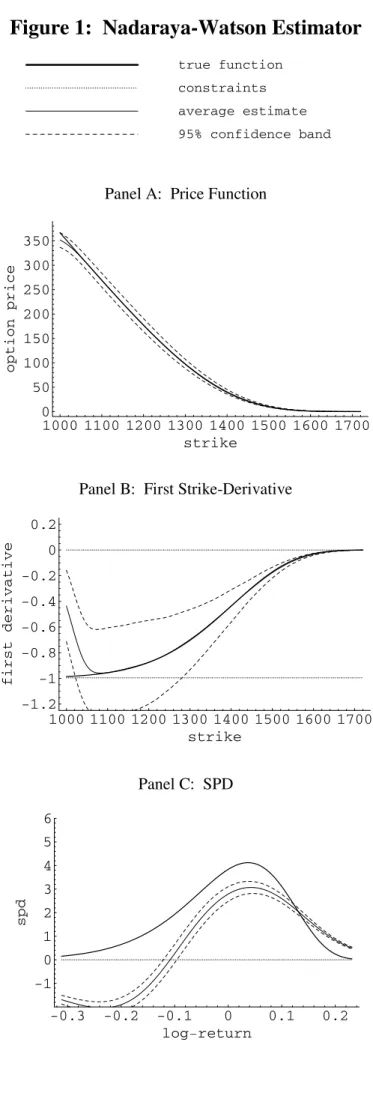
Figure 1 shows the average estimate, a 95% conÞdence interval, and the true functions for the unconstrained Nadaraya-Watson estimator. Panel A of Figure 1 shows the call pricing function estimator mˆ0,0, Panel B the Þrst derivative mˆ00,0 of the pricing function with respect to the strike price, and Panel C shows the state price densitymˆ00_0,0. As observed in Panel C of Figure 1, standard unconstrained Nadaraya-Watson estimates are, on average, negative near the left boundary, where the true probabilities are low. Of course, kernel estimation near the boundaries is known to be problematic, see e.g., Wand and Jones (1995).

Figure 2 shows the same results for the (unconstrained) locally linear estimator, mˆ0,0 in Panel A, mˆ0,1 in Panel B and mˆ00,1 in Panel C. As observed in Panel C of Figure 2, the locally linear

estimator has much lower boundary bias than the Nadaraya-Watson estimator, but the SPD still can be negative in the left boundary where the true probabilities are low.

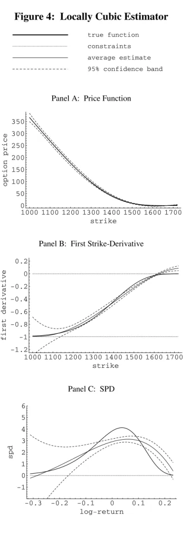
Figures 3 and 4 report the results for the locally quadratic (mˆk,2 for k = 0,1,2) and locally cubic (mˆk,3 for k = 0,1,2) estimators, respectively. As expected, higher order locally polynomial estimators perform poorly in this context because they effectively correspond to more complex local models in the absence of large enough samples. The net result is that the estimator’s biases can be entirely eliminated but at the cost of a large variance penalty. At the optimal bandwidth choice (which is what is plotted in theÞgures), the trade-offbetween squared bias and variance results in relatively large biases and variances (see Panels C in Figures 3 and 4). In addition, these estimators often violate the constraints near the boundaries (see Panels B and C). Comparing the results for the

unconstrained locally polynomial estimators corresponding to p = 0,1,2,3, it appears that locally linear estimators perform best in our context.

Figure 5 reports the results for our estimator, mˆ(0)_{, mˆ}(1) _{and mˆ}(2)_{. As observed in Panel C of} Figure 5, the constrained estimator does not share the drawbacks of the unconstrained estimators. First, the constrained SPD estimator does not have the same boundary bias as the locally constant Nadaraya-Watson —it behaves rather like the locally linear estimator that it is. Second, unlike the unconstrained locally linear estimator, the constrained estimator remains nonnegative even when the true probabilities are low. Intuitively, imposing the constraints has the effect of allowing lower bandwidths than would be optimal for a locally linear estimator in their absence. This lowers the bias of the estimator without increasing the variance correspondingly because the constraints prevent the large deviations (which would violate the constraints) from occurring. The net effect is a more accurate estimator on the basis of its mean squared error properties. Recall that we scale our density estimator and shift it, as discussed in Section 3.6. Even though these last two constraints are necessary to rule out arbitrage opportunities, our Monte-Carlo analysis reveals that, in practice, they make small difference on the estimated functionmˆ(2)(x).Indeed, for the optimal bandwidth case the average value of R₀+∞mˆ(2)(z)dz is close to one (0.94) and the average shiftz is 0.7% of the futures price.

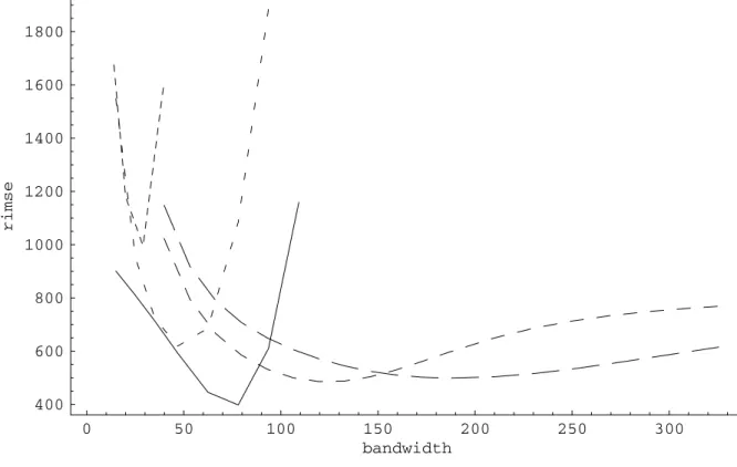
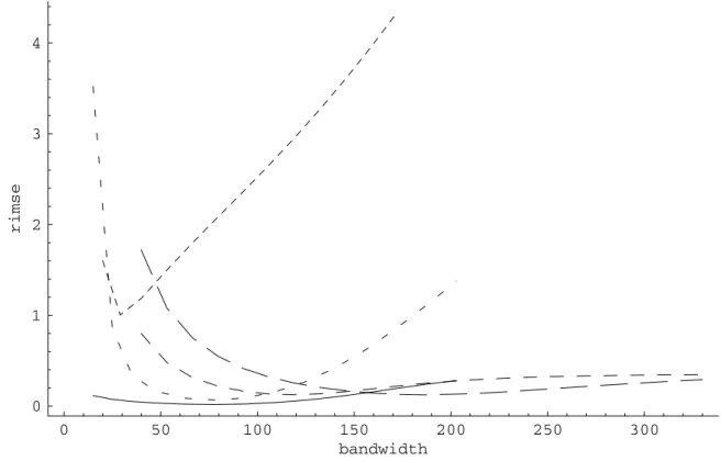
We conÞrm that intuition by studying the mean squared error behavior of the various estimators, both pointwise and global, for the sample size under consideration. Figure 6 reports the global root integrated mean squared error (RIMSE) of theÞve estimators of the pricing function, theÞrst strike-derivative and the SPD. The RIMSE is the square root of the integral given in equation (3.20). For each function to be estimated (k= 0,1,2) and estimator (p = 0,1,2,3,and shape-constrained estimator) we used the bandwidth resulting in the lowest RIMSE. The fact that smaller (resp. larger) bandwidths result in smaller (resp. larger) bias and larger (resp. smaller) variance produce these

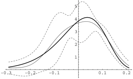
U-shaped RIMSE curves with the bottom of the U identifying for each function and estimator the globally optimal bandwidth used in Figures 1 through 5 respectively. Comparing speciÞcally our constrained estimator to the unconstrained locally linear estimator conÞrms the initial intuition: the shape-constrained estimator results in a lower RIMSE for lower bandwidths. For larger bandwidths, the two estimators converge because larger bandwidths result inßatter estimates, which consequently tend to satisfy the constraints. This explains why the RIMSE curves for these two estimators converge to one another to the right of their respective minima. However, the lowest RIMSE for the constrained estimator of the SPD is about 25% lower than that of the unconstrained estimator because lowering the bandwidth from the unconstrained optimum results in further decreases of the shape-constrained RIMSE. Figure 7 shows the local, or pointwise, effect of oversmoothing (higher bias, lower variance) and undersmoothing (lower bias, higher variance) the constrained estimator relative to the optimal bandwidth.

Furthermore, we should note that, in all likelihood, MSE-based error measures alone underesti-mate the true cost of using an estimator that can violate the constraints. The mean-squared error does not attach any penalty to violations of the constraints by the unconstrained estimators. Eco-nomic measures of the cost of violating the constraints could be quite large. For example, hedges based on option deltas that violate the constraints could quickly become ineffective; pricing with an estimated SPD that is negative in the left tail leads to underestimation of out of the money put prices, trades could be put in place based on the false perception of arbitrage (locally negative SPD), etc.

Simulation results for n = 50 observations, and the Þrst simulation design, are qualitatively similar. Overall, the results of the simulations suggest that for these types of sample sizes, imposing the shape constraints (2.5) results in a substantial improvement of the estimators.

4.2

Comparison with Parametric Alternatives

Finally, we also compare our estimator to two parametric alternatives. We consider the Jarrow and Rudd (1982) parametric extension of the Black-Scholes model where the lognormal density is replaced by a four-parameter expansion, namely

p(ST|St) = exp©₋z2_/2ª ST √ 2πτ σ ³ 1 +µ3 6 ¡ z3₋3z¢+µ4 24 ¡ z4₋6z2+ 3¢´ (4.1) where z=z(ST|St) = Ln(ST/St)− ¡ µ₁₋σ2/2¢τ σ√τ

and the call price computed as

Pt=e−rτ Z +∞

K

(ST −K)p(ST|St)dST. (4.2) The 4 parameters µ₁, σ, µ₃, µ₄ are estimated by minimizing the squared deviations between market prices and parametric prices.3 Since there is no bandwidth choice involved in this parametric formula, there is only one density per simulation. Given the sample sizes we consider, moreßexible functional forms become essentially nonparametric in nature — if we have 25 observations and we are Þtting a parametric model with, say, up to 10 parameters, then the choice of the number of parameters becomes akin to the choice of the bandwidth in nonparametrics.

The second parametric family we use in our comparisons is aÞve-parameter mixture of lognormal densities which has been used in this context by Bahra (1996). The assumed model is

p(ST|St) =αpLN(ST|St;µ1, σ1) + (1−α)pLN(ST|St;µ2, σ2) (4.3) where pLN(ST|St;µ, σ) = 1 ST √ 2πτ σexp ½ −_2σ1_2τ ¡Ln(ST/St)− ¡ µ₁₋σ2/2¢τ¢2 ¾

and the call price computed as in (4.2). The pricing formula corresponding to (4.3) is a linear com-bination of Black-Scholes formulae (αtimes the Black-Scholes formula corresponding to parameters

(µ₁, σ1) plus 1−αtimes the Black-Scholes formula corresponding to parameters (µ2, σ2)).

The 5 parametersα, µ₁, σ1, µ2, σ2are estimated by minimizing the squared percentage deviations between market prices and parametric prices. The reason for using squared price errors in one case and squared percentage errors in the other is that they produced the best results for the two methods respectively. Attempting to minimize squared price errors with the mixture of lognormals often produces nonsensical results, where one of the two densities is tailor-made to Þt in the money calls where pricing errors in dollars are costly, resulting in that density having a very low value of its σ parameter (in addition to a very negative value of itsµparameter).

Both parametric models provide a better contrast between the results of a true parametric pro-cedure and those of nonparametric ones. Panels A and B of Figure 8 report the results for the estimated SPD resulting from these two methods, in the same format as Panel C of Figures 1-5. Because they are global in nature as opposed to local, the two types of parametric estimators are unable to cope well with arbitrage violations in the data. This is not due to the inadequacy of the parametrizations: as we show in Panels C and D of Figure 8, the two models can Þt the true SPD

assumed in the data generating process (with no noise) almost perfectly. The issues arise when we attempt toÞt a set of price data that includes noise, i.e., sometimeslocal violations of convexity, as this produces aglobal distortion of the estimator — in other words, the error propagate from the local violation (which often occurs in one tail) throughout the estimated distribution (including near the peak and in the other tail).

This results in RMSE measures that, for the same simulation designs as the other estimators we considered, are worse than what can be achieved by our proposed locally linear constrained estimator. After all, avoiding this local-to-global contamination due to outliers, bad data, etc., is often why one uses nonparametric estimators in theÞrst place. Locally polynomial estimators are particularly apt at dealing with this issue.

5

Example: S&P 500 Implied SPD Under Shape Restrictions

Aït-Sahalia and Lo (1998, 2000) estimated the market call pricing function from a sample of 14,441 option prices on the S&P 500 index. They used the semiparametric approach described in (2.12). They found empirically, without imposing shape constraints, that their SPD estimator is convex but only because of the dimension reduction involved in the semiparametric speciÞcation, and because of the very large size of their sample. In practice, it would be desirable to have similar guarantees with substantially smaller samples. Indeed, as opposed to Aït-Sahalia and Lo (1998, 2000), we work with samples of tiny sizes (a typical cross-section at one point in time of 20to 30options versus a time-aggregated cross-section of 14,431options).

The data consist of the closing prices on May 13, 1999 for call options on the S&P 500 traded at the CBOE for a maturity of 65 days corresponding to the July 1999 expiration (July 17). The closing spot price of the S&P 500 on that day was 1367.56, and the risk free interest rate for that maturity was 4.83%. The dividend yield is implied through put-call parity for the put-call pair at the money. The results from applying theÞve different estimators (unconstrained Nadaraya-Watson, unconstrained locally linear, quadratic and cubic, shape-constrained locally linear) are reported in Figure 9. The bandwidths correspond to the optimum identiÞed in the previous section. The three panels correspond to the three functions to be estimated. As is apparent from Panel A, all estimators produce sensible looking (and visually indistinguishable) estimates for the pricing function as long as strikes remain relatively near the money (strikes between 1200 and 1500). However, for values of the strike price above 1600 the locally quadratic and locally cubic estimators display their high variability tendency which was clearly apparent in the simulations. And the Nadaraya-Watson estimator exhibits poor boundary behavior below 1100, clearly violating the convexity constraint on

prices.

Naturally, differentiation tends to emphasize the differences between estimators. In Panel B, all remaining estimators except the two locally linear ones (constrained and unconstrained) violate the Þrst derivative constraints somewhere. Regarding SPD estimates in Panel C, all the uncon-strained estimators either violate the positivity constraint in the left tail of the density, or are too ßat when evaluated at the globally optimal bandwidth. The unconstrained locally linear estima-tor tracks the constrained estimaestima-tor relatively closely, except that the optimal bandwidth tends to produce an estimator that is slightly too ßat, as was evidenced in the discussion of our simulation results. By contrast, the optimal amount of smoothing for the shape-constrained estimator is slightly lower which produces an estimator that is more sensitive to Þner features of the data. Indeed, our shape-constrained estimator produces an estimate of the SPD which looks quite plausible, displaying the expected level of negative skewness and excess kurtosis, while satisfying (by construction) the positivity constraint.

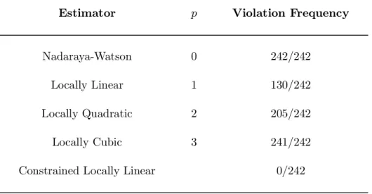
Finally, we report in Table 1 the results of repeating this analysis for every trading day during the year 1999. We repeated the analysis for different days (one set of quotes per day, each day treated separately) and report the frequency of arbitrage violations during that year. The unconstrained locally linear estimator violates the restrictions over 50% of the time, a percentage which rises to close to 100% as we move to the (unconstrained) locally quadratic and cubic estimators. By contrast, our estimator never violates the constraints (and still results in lower RMSE). The violation of the arbitrage restrictions by the unconstrained estimators hold across a large spectrum of bandwidth values. Substantial oversmoothing is required to make the unconstrained estimator no longer violates he constraints. But this then results in a large bias.

6

Conclusions

This paper proposed a method to incorporate shape restrictions, such as monotonicity and convexity, into nonparametric locally linear estimators. The estimator is motivated by the practical problem of estimating state-price densities with option data, in a setting where no information other than monotonicity and convexity is available, yet the sample size is typically small. The simulations results indicate that nonparametric estimates can be quite feasible in sample sizes as small as twenty observations, provided that appropriate theory-motivated shape restrictions, such as monotonicity, and/or convexity, are imposed. As discussed in the Introduction, this is a frequent occurrence in other areas of economics as well.

many uses. First, it provides us with an arbitrage-free method of pricing new, more complex, or less liquid securities, e.g., OTC derivatives or non-tradedßexible options, given a subset of observed and liquid “fundamental” prices, in this case basic call-option prices, that are used to estimate the SPD. We are able to achieve this in the context where very few fundamental securities are available, i.e., the observed cross-section is very sparse. Second, from a risk management perspective, our SPD estimates provide information that is crucial to understanding the nature of the fat tails of asset-return distributions implied by options data. Volatility cannot be used as a summary statistic for the entire distribution when typical return series display events that are three standard deviations from the mean approximately once a year. Our approach yields an estimate of the entire return distribution, from which single points, such as value-at-risk, can easily be derived. Third, our nonparametric estimator captures those features of the data that are most salient from an asset-pricing perspective and which ought to be incorporated into any successful parametric model. It also helps us understand what features are missed by tightly parametrized models, such as day-to-day or even intraday changes in the shape of the SPD, since we can now estimate such SPDs nonparametrically on the basis of very few observations. In fact, a nonparametric analysis can often be advocated as a prerequisite to the construction of any parsimonious parametric model, precisely because important features of the data are unlikely to be missed by nonparametric estimators.

Appendix

A

The Constrained Least Square Regression Algorithm

A.1

Transforming the Constrained Least Squares Problem to One with Conic

Constraints

We start by rewriting the constrained least squares problem in such a way as to reduce it to a convex cone problem which is then amenable to Dykstra’s algorithm for constrained least squares under conic constraints. Goldman and Ruud (1995) contain ideas along those lines, although not a formal development. Write our constraints (3.3) in matrix form as A.m₋b _≤ 0, where A is n+ 1 (the number of constraints) by n (the number of mi’s) and b is (n+ 1)×1. In its original form, our problem is therefore min m∈Rnkm−yk 2 _(A.1) subject to A.m₋b_≤0 DeÞne u=   m−y t  =   z t  , v=   0 1  , C = (A_|A.y₋b)

wheret is1_×1,and the0 block in the vector vis n_×1.Then consider the problem

min

u∈Rn+1ku−vk

2 ₌

kz_k2+_|t₋1_|2 (A.2)

subject to C.u_≤0 and t= 1

where minimizing overu means minimizing over(z, t). The solutionu∗∗_{= (z}∗∗_{,1)to problem (A.2)}

gives the solutionm∗∗ of our original problem (A.1) asm∗∗ _≡ z∗∗ +y. Indeed, the solution u∗∗ of (A.2) has set t= 1and then minimized_kz_k2 overzunder the constraint thatC.u_≤0 and we have

C.   z

1



_≤0 _⇔ A.z+ (A.y₋b)_≤0 _⇔ A.m₋b_≤0.

But problem (A.2) still does not have conic constraints (because of the constraintt = 1,which is again affine). So consider next the problem where we have relaxed the affine constraint t= 1 to

the linear (or conic) constraintt_≥0 : min

u∈Rn+1ku−vk

2

=_kz_k2+_|t₋1_|2 (A.3)

subject to C.u_≤0 and t_≥0

Now this problem is in Dykstra’s conic constraints form, and let its solution be denoted by u∗ ₌ (z∗, t∗).

Let us see how the solutions to the two problems (A.2) and (A.3) are related. Note that because u∗∗ _{satisÞes the constraint C.u}∗∗ _{≤0,we have}

A.z∗∗+ (A.y₋b)_≤0.

Since t∗_≥0,it follows that

A.z∗∗t∗+ (A.y₋b)t∗ _≤0.

Therefore (z∗∗_t∗_{, t}∗_{) satisÞes the constraints of problem (A.3). Since by deÞnition the optimum of}

problem (A.3) is reached atu∗ = (z∗, t∗),it follows that

kz∗_k2+_|t∗₋1_|2 _{≤ k}z∗∗t∗_k2+_|t∗₋1_|2

or

kz∗_k2 _{≤ k}z∗∗t∗_k2. (A.4)

Now, it is also the case that, sinceu∗ _{satisÞes the constraintC.u}∗_{≤0,we have}

A.z∗+ (A.y₋b)t∗ _≤0.

Since t∗_≥0,it follows that

A.(z∗/t∗) + (A.y₋b)_≤0,

so that ((z∗/t∗),1) satisÞes the constraints of problem (A.2). But by deÞnition the optimum of problem (A.2) is reached atu∗∗ _{= (z}∗∗_,1),thus

kz∗∗_k2 _{≤ k}(z∗/t∗)_k2. (A.5) Multiplying equation (A.5) by(t∗)2 and combining with (A.4), it follows that_kz∗_k2 = _kz∗∗t∗_k2,

so that the minimum of problem (A.2) is achieved at

z∗∗=z∗/t∗. (A.6)

Therefore the solution(z∗∗,1)of problem (A.2).can be obtained from the solution(z∗, t∗)of problem (A.3). Recall that the solution m∗∗ to our original problem (A.1) is obtained from the solution of problem (A.2) by m∗∗ _≡ z∗∗+y. Hence solving problem (A.3) using Dykstra’s algorithm to Þnd

(z∗_{, t}∗_{) ultimately gives us the the solutionm}∗∗ _{to our original problem (A.1).}

A.2

Algorithm for Constrained Least Squares Under Conic Constraints

We now brießy describe Dykstra (1983)’s algorithm to solve the constrained least square regression problem (A.3), which has conic constraints. DeÞne the following cones inRn+1_{.Forj= 1, ..., n−2,} let Cj ={u∈Rn+1 s.t. zj+2−zj+1 xj+2−xj+1− zj+1−zj xj+1−xj +t_×(yj+2−yj+1 xj+2−xj+1− yj+1−yj xj+1−xj )_≤0_} j=_{1, ..., n₋2_} and Cn−1 = {u∈Rn+1 s.t. −zn+t×(−yn)≤0} Cn = {u∈Rn+1 s.t. zn−zn−1+t×(yn−yn−1)≤0} Cn+1 = {u∈Rn+1 s.t. −z2+z1+t×(−y2+y1−(x2−x1)×e−rt,ττ)≤0} Cn+2 = {u∈Rn+1 s.t. −t≤0}.

The minimization problem (A.3) can be written as:

min u∈Tnj=1+2Cj n X i=1 (ui−vi)2 (A.7)

The algorithm consists in repeatedly projecting the vectoru onto the cones Cj :

• Letu1,1 denote the projection ofuonto the coneC1.LetI1,1 =u1,1−udenote the incremental change incurred by the projection, so thatu1,1=u+I1,1

• Let u1,2 denote the projection of u1,1 onto the cone C2. Let I1,2 = u1,2 −u1,1 denote the incremental change incurred by the projection, so thatu1,2 =u+I1,1+I1,2.

• Let u1,n+2 denote the projection of u1,n+1 onto the cone Cn+2. Let I1,n+2 = u1,n+2 −u1,n+1 denote the incremental change incurred by the projection, so that u1,n+2 = u+I1,1 +I1,2+

I1,3+....+I1,n+1+I1,n+2.

• After u1,n+2 and I1,n+2 are found. Let u2,1 denote the projection of u+I1,2...+I1,n+2 onto the cone C1. Note that we have removed the increment I1,1 before this projection. The new increment isI2,1 =u2,1−(u+I1,2...+I1,n+2).

• Continue, untilu_•,• ∈Tn+2j=1 Cj.

The projections ofu_•,• onto conesCj are easily obtained. If we represent the cone Cj by Cj = {u_∈Rn+1 _s.t.Pn+1

i=1 aj,iui≤0}, then the projection ofu ontoCj is given by:

P(u_|Cj) =    u if Pn+1_i=1 aj,iui ≤0 u0 if Pn+1_i=1 aj,iui>0 where u0_i=ui− (Pn+1_l=1 aj,lul)aj,i Pn+1 l=1 a2j,l .

B

Proof of Proposition 1

Part 1: Proof thatexp(₋rt,ττ)≤mˆ1,1(x)≤0.

The proof is based essentially on rearranging the terms in the numerators and the denominators of the locally linear estimators in such a way that they can be signed. With ki = Kh(x−xi) = h−1_K(h−1_(x−x

i)), the local linear estimator of the regression function is

ˆ m0,1(x) = βˆ0,1 = Sn,2Tn,0−Sn,1Tn,1 Sn,2Sn,0−Sn,12 = Pn i=1 Pn j=1(xj−x)2mikikj−Pni=1 Pn j=1(xj−x)(xi−x)mikikj Pn i=1 Pn j=1(xj−x)2kikj−Pni=1 Pn j=1(xi−x)(xj −x)kikj = Pn−1 i=1 Pn j=i+1(xj−xi)((xj−x)mi−(xi−x)mj)kikj Pn−1 i=1 Pn j=i+1(xi−xj)2kikj (B.1)