INSPECTION OF INTERNAL POST-TENSIONED TENDONS USING NONDESTRUCTIVE TESTING
A Thesis by
VIRGINIA RENE FOSTER
Submitted to the Office of Graduate and Professional Studies of Texas A&M University
in partial fulfillment of the requirements for the degree of MASTER OF SCIENCE
Chair of Committee, Stefan Hurlebaus Committee Members, Mary Beth Hueste
Robert Warden Head of Department, Robin Autenrieth
December 2016
Major Subject: Civil Engineering
ii
ABSTRACT
Post-tensioned (PT) bridge systems have been used for many years and are generally favored by contractors and engineers. This is because they are economical, can be used for long spans, increase the structural capacity, and are fairly easy to construct. In these systems, the structural integrity of the PT tendons is critical. To protect the steel strands, a cementous grout material is injected into the ducts. However, the presence of grout voids in the tendons combined with the ingress of chlorides allows for corrosion of the steel strands. Additionally, the use of low-quality grout can cause extreme local pitting. This corrosion has a detrimental effect on the structural integrity of the bridge girder. Numerous tendon failures have occurred world-wide which have been attributed to these grout defects. The condition of the PT tendons must be monitored to ensure public safety. This research investigates the use of ultrasonic tomography (UST), ground penetrating radar (GPR), and infrared thermography (IRT) to evaluate the grout condition of internal PT tendons.
A 75-ft (22.86 m) bridge girder was constructed at the Texas A&M Riverside Campus. A complex defect design was developed and implemented. The defects include grout voids and water-filled cavities of varying sizes, as well as several grout conditions, including soft grout, unhydrated grout, and gassed grout. To test the
capabilities and limitations of the various non-destructive testing (NDT) techniques, both metal and plastic ducts were utilized. The results suggest that UST may be able to identify sizeable water-filled cavities when metal ducts are utilized. However, strong
iii
reflections from plastic ducts make the grout defects unidentifiable. While GPR is able to detect the duct location, it is unable to identify any grout defects, regardless of the duct material. The internal ducts are embedded too deep into the girder walls for IRT to detect grout voids within the tendons. However, it showed promising results when inspecting the end caps, correctly identifying nearly 95% of grout voids in the anchorage regions.
iv
DEDICATION
This thesis is dedicated to my mother and father for their continued love, patience, and support. Words cannot express the amount of gratitude I wish to extend. They have worked immense hours and made great sacrifices in order to give my brother and me the opportunity to pursue our dreams. They have been in the trenches with me not just throughout my academic career but every single day of my life, celebrating my successes and encouraging me during my failures. I love you. Thank you for molding me into the person I am and for giving me the opportunity to find my place in this world.
v
ACKNOWLEDGEMENTS
I would like to thank my committee chair, Dr. Hurlebaus, for his continued encouragement and unwavering support. His dedication to his students is unrivaled.
I would also like to thank Dr. Hueste and Mr. Warden for serving on my committee and for offering their time, knowledge, and guidance.
I would like to extend a special thanks to the department faculty for their
friendship and the knowledge they have bestowed upon me. The challenging curriculum and, at times, overwhelming workload make the completion of this degree bittersweet.
Thanks are owed to Laura Byrd for her dedication to all of the graduate students in the department and her overwhelming desire to see us succeed.
vi NOMENCLATURE PT Post-tensioned NDT Non-destructive Testing CT Computerized Tomography IE Impact Echo
UPE Ultrasonic Pulse Echo
UPV Ultrasonic Pulse Velocity
UST Ultrasonic Tomography
DPC Dry Point Contact
GPR Ground Penetrating Radar
IRT Infrared Thermography
HDPE High-density polyethylene
vii TABLE OF CONTENTS Page ABSTRACT ... ii DEDICATION... iv ACKNOWLEDGEMENTS ... v NOMENCLATURE ... vi
TABLE OF CONTENTS ... vii
LIST OF FIGURES ... ix LIST OF TABLES ... xi CHAPTER I INTRODUCTION ... 1 1.1 Background Information ... 1 1.2 Research Objectives ... 5 1.3 Organization of Thesis ... 5
CHAPTER II LITERATURE REVIEW ... 7
2.1 Introduction... 7
2.2 Computerized Tomography Technique ... 7
2.3 Impact Echo Technique ... 9
2.4 Ultrasonic Technique ... 13
2.5 Ground Penetrating Radar Technique ... 16
2.6 Infrared Thermography Technique ... 19
CHAPTER III CHOSEN NDT METHODS AND TEST SPECIMEN ... 24
3.1 Chosen NDT Methods ... 24
3.2 Equipment ... 24
3.3 Test Specimen ... 27
CHAPTER IV ULTRASONIC TOMOGRAPHY ... 32
4.1 Introduction... 32
4.2 Procedure ... 32
viii
4.4 Deviator Results ... 39
4.5 Summary ... 40
CHAPTER V GROUND PENETRATING RADAR ... 42
5.1 Introduction... 42
5.2 Procedure ... 42
5.3 Girder Wall Results ... 42
5.4 Deviator Results ... 46
5.5 Summary ... 46
CHAPTER VI INFRARED THERMOGRAPHY ... 48
6.1 Introduction... 48
6.2 Procedure ... 48
6.3 Results ... 49
6.4 Summary ... 63
CHAPTER VII CONCLUSIONS & FUTURE RESEARCH ... 67
7.1 Conclusions... 67
7.2 Future Research ... 69
REFERENCES ... 72
APPENDIX A TABLES ... 75
ix
LIST OF FIGURES
Page
Figure 2-1: UPV Transducer Orientation ... 14
Figure 2-2: GPR Void Orientation ... 18
Figure 2-3: Void Orientation ... 22
Figure 3-1: MIRA A1040 Ultrasonic Tomographer ... 25
Figure 3-2: GSSI StructureScan Mini HR Device ... 26
Figure 3-3: FLIR T640 Device ... 26
Figure 3-4: Mock-up Bridge Specimen ... 27
Figure 3-5: Girder Construction Details ... 28
Figure 3-6: Internal Tendon Defect Keys ... 31
Figure 4-1: North Wall Exterior Scans – MIRA ... 35
Figure 4-2: North Wall Interior Scans – MIRA ... 36
Figure 4-3: South Wall Exterior Scans – MIRA ... 37
Figure 4-4: South Wall Interior Scans – MIRA ... 38
Figure 4-5: Deviator Scans – MIRA Device Oriented Parallel to Ducts ... 39
Figure 4-6: Deviator Scans – MIRA Device Oriented Perpendicular to Ducts ... 40
Figure 5-1: North Wall Scans – GPR ... 44
Figure 5-2: South Wall Scans – GPR ... 45
Figure 5-3: Deviator Scans – GPR ... 46
Figure 6-1: North Wall Exterior IRT Image ... 50
Figure 6-2: North Wall Images – IRT... 52
Figure 6-3: South Wall Exterior IRT Image ... 54
x
Figure 6-5: East End Cap Images – IRT ... 58
Figure 6-6: East End Cap Images – IRT ... 59
Figure 6-7: West End Cap Images – IRT ... 61
Figure 6-8: Close-up of End Caps T18 and T20 ... 62
xi
LIST OF TABLES
Page
Table 3-1: Internal Duct Specification by Tendon ... 29
Table 3-2: Grout Defect Marker and Description ... 30
Table 4-1: UST Scanning & Processing Times ... 41
Table 5-1: GPR Scanning & Processing Times ... 47
Table 6-1: IRT Collection & Processing Times ... 63
Table 6-2: Summary of IRT Results in Anchorage Regions ... 64
1
CHAPTER I INTRODUCTION
1.1Background Information
Post-tensioned (PT) systems have been widely used in bridge construction since the late 1950’s (Tinkey et al., 2007). They are favored by designers and contractors because they are economical, can be used for long spans, increase the structural capacity, and are fairly easy to construct (Im et al., 2012). Concrete specimens usually fail in tension, as its tensile strength is only about 10% of its compressive strength. PT systems become advantageous because they put the regions of the structural element which will experience tensile stresses into compression (Nurnberger, 2002). This is accomplished by placing tendons in ducts during construction. Some of these ducts may be internal, and some may be external. Once the concrete has hardened, the tendons are pulled into tension, resulting in a compressive force in the concrete element (Im et al. 2012, Nurnberger 2002).
It was once believed that PT systems are maintenance free with a service life of 120 years (Martin et al., 2001). However, this is not necessarily the case. While the PT strands are placed in ducts and cementous materials are grouted around the regions between the strands, this has not completely prevented incidences of corrosion. This corrosion has a detrimental effect on the structural capacity of PT bridges (Im et al., 2012). Minh et al. (2007) investigated the effect of tendon corrosion on the load
2
strands causes a considerable decrease in the pre-stressing force of the tendons.
Additionally, corrosion of the tendon duct decreases the bond between the concrete and the duct and significantly reduces the load carrying capacity (Minh et al., 2007). In fact, “a 25% reduction in strand capacity can result in 50% or more reduction in the live load carrying capacity of a bridge”; this has led some researchers to develop models assessing the residual strength of deteriorating PT bridges while others try to evaluate the
condition of the strands (Cavell et al. 2001, Gardoni et al. 2009, Mietz et al. 2007). The corrosion has been attributed to two sources. The first is segregated cement grout. It has been well documented that strands in contact with segregated grout
containing a “white, unhardened paste”, an exudation product of cement grout, experience deep penetrating corrosion. The high levels of water, high content of sulphate ions, and high pH (in the order of 13 or 14) is extremely corrosive to the steel strands (Bore et al. 2010, Carsana et al. 2014). The severe local corrosion causes pitting and stress concentration in these notches which can lead to a sudden and brittle fracture of the PT strands (Nurnberger, 2002). In one instance, it caused an external tendon to rupture in less than two years after construction (Bore et al. 2010, Carsana et al. 2014).
The second, more prominent, cause for corrosion is the presence of grout voids. These voids are formed by “entrapped air pockets, grout bleeding, improper grouting, or all three” (Im et al., 2010). Voids can arise if the air vents are shut off before the duct is completely filed with grout or as entrapped air moves to the high points of the duct, which are usually located near the anchorage zones (Cavell et al., 2001). In other instances, water bleeds from the grout, enters the space between the wire strands, and
3
moves towards the anchorage regions, where it collects and evaporates (Hansen, 2007). Regardless of how they are formed, these voids cause two problems. For one, the strands are unprotected and therefore susceptible to corrosion, particularly from the ingress of chlorides at the anchorage zones (Cavell et al., 2001). These chlorides come from various sources including de-icing road salts or seawater (Nurnberger, 2002). In Japan, the chlorides come from airborne salt from the sea and from the sand used to make the concrete itself (Minh et al., 2007). Secondly, a grout void does not allow for proper redistribution of stress. That is, if a strand breaks, its load cannot be properly transferred to the other strands without proper grouting (Martin et al., 2001).
The first catastrophe was the collapse of the Bricton Meadows Footbridge in the UK in 1967. Then in 1985, the Ynys-y-Gwas Bridge in Wales collapsed, only six months after a safety inspection revealed no signs of distress. Both of these failures have been attributed to the corrosion of the tension strands in the presence of grout voids (Tinkey et al., 2007). Immense concern over the safety of PT bridges in the UK caused the Department of Transport to ban their construction from 1992 until 1996 (Cavell et al., 2001). In the United States between 1999 and 2000, the Niles Channel Bridge, the Mid-Bay Bridge, and the Sunshine Skyway bridge all experienced corrosion induced tendon failures. These failures were attributed to the presence of moisture and chlorides inside voids. These failures occurred when the bridges were still quite new, only 16, 8, and 13 years after construction, respectively (Cavell et al., 2001). Inspections revealed that tendon problems existed in at least 17 additional bridges in Florida and several along the East Coast, all in use at the time (Hansen 2007, Tinkey et al. 2007). In 2001,
4
the use of a small camera revealed voids in the tendons of the Varina-Enon Bridge in Virginia. However, no significant corrosion was visible. The choice was made to fill the voids with a new high-performance grout that the American Segmental Bridge Institute promoted in place of the old Portland cement grout, which had been used until 2000. The new grout was said not to bleed nor leave voids, and the repair was completed in 2004. In May of 2007, a repaired external tendon failed after experiencing extensive corrosion (Hansen, 2007).
The growing concern over the safety of PT bridges has become world-wide. A Japanese study found that 35% of their PT systems contain voids. Another study found that 19% of the bridges inspected in the United States contain voids and that of the thousand PT bridges inspected in the UK, 30% of the ducts contained voids (Im et al., 2010). Over 100,000 bridges in China are in severe condition, and as of 2012, more than 9 billion RMB ($1.2 billion) had been spent on bridge maintenance, repairs, and
retrofitting. Maintenance funding has reached over 200 million RMB ($26 million) per year (Zhi-feng et al., 2012).
What makes the failure of PT bridges concerning is there is usually no visible evidence of distress prior to tendon rupture. Visual inspections for rust stains, spalling, and cracking are inadequate (Im et al. 2012, Tinkey et al. 2007). This has lead
researchers to explore new, more effective and efficient methods to determine the grout condition in PT tendons and assess the condition of the strands. This is essential in order to evaluate the structural integrity of the deteriorating PT bridges and ensure public safety.
5
1.2Research Objectives
The objectives of this research are:
• Determine which non-destructive testing (NDT) methods are suitable for the identification of grout voids in internal PT ducts (both metal and plastic)
• Conduct a blind test in the field using each of the selected methods
• Evaluate the overall performance of each of the selected methods
While various NDT methods exist, they may not all be applicable to internal PT duct inspection. Thus, it will be necessary to review the literature and determine which methods show promise. Several factors will be considered when selecting methods for further investigation. These include: reliability, safety, availability of the equipment, measurement speed, ease of application, and originality.
1.3Organization of Thesis
This thesis is divided into seven chapters. Chapter I gives a background into PT systems and the problems arising from strand corrosion, states the objectives of this research, and defines the structure of the thesis. Chapter II provides a literature review of several NDT methods which may be applicable to internal PT duct inspection and the previous research that has been conducted. Chapter III identifies the methods selected for further inspection and details both the chosen equipment and the test specimen. The results of the in-field tests are given in Chapter IV, Chapter V, and Chapter VI. Chapter
6
IV details the procedure and results using Ultrasonic Tomography, while Chapter V and Chapter VI detail the results using Ground Penetrating Radar and Infrared
Thermography, respectively. Chapter VII presents the conclusions from the research and offers areas for further investigation.
7
CHAPTER II LITERATURE REVIEW
2.1Introduction
While both internal and external tendons are subject to the detrimental effects of grout voids, the internal tendons pose an added element of difficulty, as they are
completely encased in concrete. That is, not only are the stands hidden from view, but the ducts themselves are not visible either. This chapter explores various
non-destructive testing (NDT) procedures considered by researchers and reviews some of the research that has been conducted to investigate the condition of internal PT tendons.
Although specifically interested in investigating external PT tendons, several of the NDT methods reviewed by Im et al. (2010) could be applicable for internal tendon inspection. These include the Computerized Tomography Technique, Impact Echo Technique, and Ultrasonic Technique. Other methods to consider include the Ground Penetrating Radar Technique and the Infrared Thermography Technique.
2.2Computerized Tomography Technique
The Computerized Tomography (CT) method uses x-ray or gamma-ray to obtain a cross-sectional image of a specimen. The use of gamma-rays to inspect concrete specimens was first reported by Mullins and Pearson in 1949 (Frigerio et al., 2004). Since that time, however, great advancements have been made in the field of
8
the gamma rays, which then had to undergo a time-consuming chemical development process. However, computerized tomography utilizes reusable image plates that are read by a scanner. This means that the data are available digitally without the use of a
chemical development process. Additionally, the CT method “provides a superior range of detectable gamma ray intensities and higher detection efficiency” (Mariscotti et al., 2009). This increases safety as it decreases the radiation exposure times and allows researchers to use a weaker, lower energy source.
Because the CT method provides an internal image of the test specimen and is extremely precise, it is considered superior to other NDT methods. In fact, it can
determine the diameter and location of reinforcement with 1/32 in. (0.79 mm) and 3/8 in. (9.53 mm) precision respectively (Frigerio et al., 2004). Because the absorption of gamma-rays is sensitive to density, the corrosion of steel reinforcement can be identified in gammagraphies. Mariscotti et al. (2009) has applied the CT method to hundreds of cases to both characterize reinforcement and determine its condition. However, not only has the CT method been used to determine the internal structure of bridge beams and identify rebar, corrosion, and honeycombing, but it has also been used to inspect PT tendons (Frigerio et al. 2004, Mariscotti et al., 2009).
Pimentel et al. (2010) conducted a gammagraphic study to inspect the PT tendon condition of the N.S. da Guia Bridge. While they were unable to identify any grout defects, wire breaks, or section loss, they were able to determine the size of both the ducts and the individual strands. However, other researchers have obtained much more promising results. Mariscotti et al. (2008) inspected a PT girder from the Zarate bridge
9
in Argentina. The girder was inspected using gamma rays from a 93Ci192Ir source. Researchers were able to identify four grouting voids and estimate their sizes. The Regional Transport Research Laboratory (LRPC) in France has had such success with gammagraphy, that it is considered the established, reliable NDT method with which to determine grout quality and condition. In fact, when the LRPC obtained a PT beam from the Pont Neuf bridge in France and sought to investigate the capabilities of other NDT methods, they used gammagraphy to identify regions for further inspection (Dérobert et al., 2002).
According to Tinkey and Olson (2007), radiography is the oldest, most successful technique in assessing grout condition. However, despite the advances in radiography, this method still suffers from many disadvantages. The technique is not ideal for in the field testing, as the test area is usually small, making the inspection very time consuming. Public safety is also a concern, as it requires the use of radiation protection, and the technique usually requires access to both sides of the specimen, making its application impractical (Dérobert et al. 2002, Im et al. 2012, Im et al. 2010, Tinkey et al. 2007).
2.3Impact Echo Technique
The Impact Echo (IE) technique involves dynamically exciting a concrete structure by striking it with a small mechanical impactor. The reflected wave energy is then measured with the use of a displacement transducer (Tinkey et al., 2007). If the
P-10
wave speed in the specimen 𝐶𝐶𝑝𝑝 is known, the echo depth 𝑇𝑇 can be computed by the following equation:
𝑇𝑇= 0.96𝐶𝐶𝑝𝑝∆𝑡𝑡2 (1)
where ∆𝑡𝑡 is the travel time from the initiation of the pulse to the arrival of the first P-wave reflection (Carino et al., 1992)
Using a Fast Fourier Transform (FFT), the displacement information collected in the time domain can be converted to the frequency domain. It has been observed that a shift downward in the thickness resonance frequency (𝑓𝑓𝑇𝑇 = 1/∆𝑡𝑡) or similarly, an increase in the apparent echo depth, 𝑇𝑇, is indicative of grout voids. That is, the grout void acts a hole, decreasing the stiffness of the specimen and therefore decreasing the dominant peak frequency (Abraham et al. 2011, Jaeger et al. 1996, Jaeger et al. 1997, Tinkey et al. 2007). Plots can be generated using the echo depth calculated using Equation (1).
The IE method shows promise, as it “produces a better noise to signal ratio than other ultrasonic techniques because of its low attenuation in composite materials” (Im et al., 2010). However, the method is rather time consuming, and it is incapable of
identifying voids partially filled with water (Im et al., 2010). Im et al. (2012) found that IE can be ineffective in detecting grout voids if an imperfect bond exists between the HDPE ducts and the grout, as these small discontinuities obstruct the elastic waves. This result is attributed to the type of grout utilized. In an effort to explore the effect of grout bleeding, Class A grout was employed in this research. However, the corresponding
11
grout shrinkage can leave tiny gaps between the ducts and the grout and prevent the propagation of the elastic waves (Im et al., 2012). Other researchers have had some success when investigating internal ducts with this technique.
Carino and Sansalone (1992) conducted a small feasibility study on a 19.7-in. (0.5-m) thick concrete slab. A 3.94-in. (100-mm) diameter metal duct was placed in the slab with a concrete cover of 5.91 in. (150 mm). Half of the duct was filled with grout while the other half remained hollow. The location of the voided duct was
experimentally calculated to be 5.12 in. (130 mm) from the top surface (Carino et al., 1992). To explore the limitations of the IE method, they then tested a 39.37-in. (1-m) thick concrete slab containing seven metal ducts. This specimen contained voids which were relatively small compared to the duct depth, used close spacing of ducts,
overlapping ducts, and three layers of rebar. However, despite the extreme testing conditions and some discrepancies between the experimental results and the actual test specimen, the results were promising. Abraham et al. (2011) observed similar results while also exploring the frequency shift due to the local stiffness of a specimen, the effect of thick walled ducts, and epoxy-filled ducts.
Jaeger et al. (1996) took a slightly different approach, conducting both numerical and experimental studies to determine if the IE method could be used to identify partial and complete grout voids. The researchers sought to understand the interaction between PT tendons and the transient stress wave. Ultimately, they determined that a thin metal PT duct is transparent to incident waves and were able to characterize the frequency-domain signal of a solid plate, a grouted duct, and an ungrouted duct. The researchers
12
then used these observations to conduct a field test on a PT bridge. Of the 14 steel tendon ducts inspected, the IE method found that eleven were completely grouted and that three contained grout voids. After the NDT inspections were complete, the ducts were physically opened, and the grout condition was visually inspected. The IE method was accurate in all cases. However, one of the ducts which was identified to have a grout void was partially grouted; that is, the size of the void was unknown until physically opening the duct (Jaeger et al., 1997).
The main disadvantage to IE is the testing speed (Carino et al. 1992, Im et al. 2010). To address this issue, Tinkey and Olson (2007) developed a rolling scanner which allows for “rapid testing”. If the test specimen is smooth, no coupling agent is required. This scanner was used to scan two specimens. The first was a 100-ft (30.48-m) mock-up U-shaped bridge girder containing eight steel ducts. Grout voids of varying sizes were simulated using stepped and tapered Styrofoam rods. Again, there was fairly good agreement between the experimental results and the true defect design. There were some discrepancies, as a few voids were identified where they were not intentionally placed. Similarly, there were regions that appeared fully grouted where Styrofoam voids were placed. However, in general, the results were impressive. Grout voids as small as 9% depth loss (20% circumferential diameter loss) were able to be identified in a 4-in. (101.6 mm) steel duct. The authors suggest using x-ray to verify the realization of the defect design and to explain any of these discrepancies. The second specimen was a mock-up slab which contained eleven metal ducts. The condition of the ducts varied greatly. These differences included the size of the duct, the amount of concrete cover,
13
the size of defects, and the number of wire strands. The results from scanning the slab were similar, and revealed two limitations of the IE method. The greater the concrete cover, the harder the defects are to detect, particularly when the ducts are small.
2.4Ultrasonic Technique
Ultrasonic techniques are acoustic methods which use sound waves with a frequency of 18 kHz and higher (Im et al., 2012). The elastic waves travel through a medium by the progressive vibration of particles (Hoegh, 2013). Regardless of which method is utilized, the basic premise is as follows: A transducer generates a stress pulse which travels through the specimen and interacts with its internal structure. The wave is reflected at material interfaces due a change in density, or similarly the acoustic
impedance. The amount of reflection is directly related to the acoustic impedance differential between the two materials; that is, the greater the contrast, the greater the reflection. A transducer, acting as a receiver, then records the reflected wave. Using the time-of-flight of the ultrasonic pulse, information about the specimen’s internal
condition can be assessed (Hoegh, 2013).
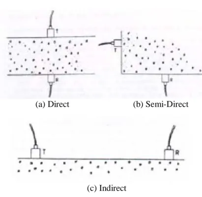
There are several types of ultrasonic testing systems. The Ultrasonic Pulse Echo (UPE) method uses a single transducer which acts as both the transmitter and receiver, whereas the Ultrasonic Pulse Velocity (UPV) method employs two transducers. One transducer acts as the transmitter and the other as the receiver (Im et al., 2010). The orientation of the transducers can be direct, semi-direct, or indirect, as detailed in Figure 2-1.
14
(a) Direct (b) Semi-Direct
(c) Indirect
Figure 2-1: UPV Transducer Orientation (Hoegh, 2013)
However, there are numerous issues that arise using the traditional UPV method, as the results are highly sensitive to small shifts in the locations of the transducers. This has led to the development of ultrasonic array technology. This alleviates some of the issues with the ultrasonic technique, as it provides consistency in transducer pair spacing and reduces signal variability, thus improving the reliability of test results (Hoegh, 2013). Ultrasonic Tomography (UST) involves “measuring the time-of-flight of an ultrasonic pulse along many ray paths” through a specimen (Martin et al., 2001). The mathematical theory dates back to 1917 and shows that the internal characteristics of a specimen can be reconstructed, given a complete set of projections through the object (Martin et al., 2001).
15
To test the plausibility of using ultrasonics to identify grout voids in external PT tendons, Im et al. (2012) set up 16 test specimens. The pitch-catch method of UPV was utilized, in which the transmitting and receiving transducers are on the same side of the specimen. This is also known as the indirect method and is illustrated in Figure 2-1c. Ultimately, this method has proven impractical and inefficient in testing external ducts for grout voids, as it was incapable of differentiating between voids and tiny gaps caused by an imperfect bond between the grout and HDPE duct. These results are attributed to the type of grout used in the experiments and the corresponding shrinkage. Additionally, traditional piezoelectric contact transducers require the use of a couplant, and the UPV method can be quite time consuming (Im et al., 2010). Other ultrasonic studies
conducted on internal PT ducts, however, show promise.
Martin et al. (2001) used UST to test a beam containing two 3.94-in. (100-mm) metal PT ducts. A tomographic grid was set up on the sides and top surface of the beam using numerous transducers spaced 3.94 in. (100 mm) apart. Cross-sectional images were obtained at three points along the length of the specimen. This experiment yielded fairly good results. However, the author notes the need for a more refined test grid, requiring even more transducers (Martin et al., 2001). Although the method employed by Martin et al. (2001) yielded good results, the procedure does suffer a few
disadvantages. Mainly, the need for many transducers makes it expensive. However, UST is believed to be a promising method provided some of the limitations be
16
One of the main limitations of ultrasonic methods is the requirement of a
coupling agent. A liquid couplant is often utilized between the transducer and specimen to assist in the transmission of the elastic wave, which cannot propagate through air efficiently. The development of low frequency, dry point contact (DPC) transducers has not only eliminated the need of a coupling agent, but also allowed for greater penetration depths (Hoegh, 2013). Williams (2014) used a phased-array UST device to identify voids, water infiltration, structural elements, cracks, and delaminations in concrete tunnel linings. The transverse transducers are dry contact and the results are reliable. This new UST device may be useful in identifying grout voids in internal PT ducts.
2.5Ground Penetrating Radar Technique
Ground Penetrating Radar (GPR) has proven to be a reliable NDT method with various applications in the civil engineering field. It has been successfully used in concrete void detection and the inspection of concrete linings (Williams 2014, Zhi-feng et al. 2012). GPR functions as follows: Electromagnetic waves are emitted from a transmitter antenna; the waves travel through the specimen, and are reflected at material interfaces due to a change in dielectric properties. The reflected waves are then detected by a receiver antenna. The amount of the wave that is reflected at the material interface depends on the contrast in the dielectric permittivity of the two materials. That is, the greater the contrast, the greater the reflection. The reflection coefficient, 𝑅𝑅, can be computed as:
17 𝑅𝑅 = 𝑣𝑣2−𝑣𝑣1
𝑣𝑣2+𝑣𝑣1 =
√𝜀𝜀2−√𝜀𝜀1
√𝜀𝜀2+√𝜀𝜀1 (2)
where 𝑣𝑣1 and 𝑣𝑣2 are the radiowave velocities of Material 1 and Material 2
respectively and 𝜀𝜀1 and 𝜀𝜀2 are the respective relative dielectric permittivities (Zhi-feng et al., 2012).
From Equation (2), it is apparent that the reflection coefficient can be negative or positive. If the wave travels from a medium with a higher dielectric constant to one with a lower dielectric constant, the reflection coefficient is negative. This corresponds to a phase change of the electromagnetic wave upon reflection. This occurs, for example, if the wave travels from concrete to air (i.e. a void is detected). If the wave travels from a material with a lower dielectric permittivity to a material with a higher dielectric
permittivity, then the wave experiences no phase change and the reflection coefficient is positive. This occurs if the wave travels from concrete to steel (i.e. rebar is detected). Thus, the sign of the reflection coefficient can be used to identify objects within a specimen (Zhi-feng et al., 2012).
Zhi-feng et al. (2012) experimented with GPR to test for grout voids in internal PT ducts. A small scale test specimen was created which contained both a plastic and a metal duct, 3.94 in. (100 mm) in diameter. The concrete cover was 1.96 in. (50 mm). A variety of soft foams were used to simulate grout voids. Ultimately, the researchers were able to identify the presence of voids in the plastic ducts. However, the voids in the metal ducts were not able to be identified as they produced “great electromagnetic shielding functions” which prevented the electromagnetic waves from propagating into
18
the ducts (Zhi-feng et al., 2012). Because most PT bridges constructed before the mid 1990’s were constructed using metal ducts, this could limit the application of GPR (Martin et al., 2001).
Pollock et al. (2008) also investigated the plausibility of using GPR to identify PT tendons and voids. Using a 1.5 GHz GPR system, they scanned 14 specimens varying in thickness. Ultimately, they were unable to identify any of the simulated voids in the steel ducts, consistent with previous research. However, the general location of the steel ducts, their size, and depth in the specimen were all accurately determined. The plastic ducts were identifiable, as were the simulated voids, given that the voids were oriented properly; that is, if the voids were located between the steel strands and the face of the specimen, as in Figure 2-2a, they were identifiable. However, if the voids were oriented as in Figure 2-2b, where the voids were adjacent to the steel strands, they were undetectable.
(a) Identifiable Void Orientation (b) Unidentifiable Void Orientation
19
Pollock et al. (2008) also note that the location of the ducts immensely effects whether or not they are detectable. The deeper the ducts are embedded, the weaker the reflections and the lower the image quality. Additionally, if the ducts are located too close to the top layer of reinforcement, it might have a “masking effect” on the detection of voids (Pollock et al., 2008).
2.6Infrared Thermography Technique
Infrared Thermography (IRT) is a very rapid NDT method that has been used in various civil applications, from inspecting bridge decks to concrete tunnel linings. Thermal imaging cameras can detect the thermal energy emitted from a specimen and convert it into an electrical signal, producing a thermal image (Pollock et al., 2008). The hotter an object is, the more infrared radiation it emits. As heat propagates through a specimen, any defects or voids will affect the transfer of thermal energy, as they have different rates of heat conduction than the surrounding concrete (Pollock et al., 2008). This will cause surface temperature variations which will be visible in the thermal image (Musgrove 2006, Williams et al. 2015).
A temperature gradient through the thickness of the specimen is mandatory for the IRT technique, as it induces the heat flow (Musgrove, 2006). There are various heat sources which can be utilized to obtain the required temperature gradient. These include the use of heating blankets, infrared heaters, and solar energy.
Musgrove (2006) used infrared thermography to detect PT tendons and simulated voids in concrete specimens. Eight rectangular concrete specimens were constructed,
20
each measuring 40 in. (1016 mm) by 64 in. (1625.6 mm). These slabs varied in thickness, duct material, concrete cover, and the number of steel strands and voids per duct. Before conducting any experiments, he developed 2-dimensional finite element models of heat flow through the cross-section of each specimen. He considered both insulated and uninsulated boundary conditions with temperature loading on a single surface. He also created models with and without voids to quantify the effect voids have on surface temperature. These models would provide the required thermal conditions necessary to detect tendons and voids.
According to the finite element models, detecting tendons in a 16 in. (406.4 mm) thick specimen would require an applied temperature of at least 500ºF (260ºC) or a temperature gradient of 425ºF (236ºC). Because of these extreme temperature
requirements, Musgrove (2006) decided to conduct physical experiments on only the 8 in. (203.2 mm) and 12 in. (304.8 mm) thick specimens. He considered three different heat sources, including solar energy, electric silicone rubber flexible heating blankets, and an infrared heater.
Ultimately, Musgrove (2006) was able to detect tendons and voids in the 8 in. (203.2 mm) specimens with a temperature differential of 20ºF (11.1ºC) given that the concrete cover was less than 2 in. (50.8 mm). HDPE ducts with low amounts of steel and steel ducts with large amounts of steel were the easiest to detect due to the large change in thermal conductivity. HDPE ducts with large amounts of steel were difficult to detect because the higher thermal conductivity of the steel is offset by the low thermal
21
conductivity of the plastic duct. Steel ducts with small amounts of steel were also difficult to detect.
The 12 in. (304.8 mm) thick specimens required much higher temperature gradients in order to detect tendons and voids. The only tendons that were detectable were those which caused a large difference in heat flow through the specimen. Tendons with a cover depth up to 6 in. (152.4 mm) were detectable with a temperature gradient of at least 135ºF (75ºC). At these temperatures, simulated voids could be detected with concrete covers of 2 in. (50.8 mm) or less.
Pollock et al. (2008) also experimented with thermal imaging. They considered three different methods. The first method was to direct an infrared heater at one face while recording thermal images of the unheated face. The second method was to direct the infrared heater at one face and take thermal images of the heated surface. The third method utilized solar energy, and thermal images were taken of the heated surface. Ten rectangular specimens were inspected using the methods described above. These specimens varied in thickness, duct material, concrete cover, and the number of steel strands and voids.
Simulated voids were detectable in the 8 in. (203.2 mm) specimens. The first method was most successful, identifying every tendon and most voids. The third method also provided some useful results, identifying voids two of the three times it was
utilized. However, while the PT tendons were usually detectable in the 12 in. (304.8 mm) specimens using the first method, a void was detected in only one instance.
22
Pollock et al. (2008) also discovered that the orientation of the void was critical to its detection. Images of the two different void orientations appear in Figure 2-3.
(a) Unidentifiable Void Orientation (b) Identifiable Void Orientation
Figure 2-3: Void Orientation (Pollock et al., 2008)
Only the voids orientated as in Figure 2-3b were detectable, when the void was positioned between steel tendon and the infrared camera. Voids orientated as in Figure 2-3a were not detectable because “the heat could bypass the voids by propagating though the adjacent tendons” (Pollock et al., 2008).
Additionally, Pollock et al. (2008) were only able to detect simulated voids in plastic ducts; that is, none of the simulated voids in steel ducts were identified. It is believed that most of the heat is transferred through the steel ducts, bypassing the simulated void. This observation seems consistent with the results obtained by
Musgrove (2006); when steel ducts were utilized, simulated voids were only detected in one instance.
Pollock et al. (2008) inspected a PT concrete box girder with 12 in. (304.8 mm) thick walls using both the first and second testing methods. Despite the success in the
23
small scale studies, none of the PT ducts were visible in the box girder. The thicker concrete makes it difficult to obtain a sufficient temperature gradient between the heated and unheated surfaces. The heat not only propagates through the wall thickness, but also along the length and height of the specimen. While this allows surface conditions to be evaluated, the internal conditions cannot be determined (Pollock et al., 2008).
24
CHAPTER III
CHOSEN NDT METHODS AND TEST SPECIMEN
3.1Chosen NDT Methods
Of the reviewed methods, three were selected for further exploration. These include Ultrasonic Tomography, Ground Penetrating Radar, and Infrared Thermography. These methods have proven to be reliable, safe, and easy to implement. Additionally, these methods can be executed with reasonable inspection times. GPR is not terribly time consuming nor is UST when compared to traditional ultrasonic methods. Furthermore, Infrared Thermography is an extremely quick inspection technique.
3.2Equipment
The MIRA 1040A Ultrasonic Tomographer has been selected to implement the ultrasonic testing, shown in Figure 3-1a. The device has a 4 by 12 array of
low-frequency broadband transverse transducers. These transducers are dry contract, have wear-resistant ceramic tips, and are spring loaded. Each row of transducers progressively emits shear waves while the remaining rows function as receivers. This process is illustrated in Figure 3-1b. The ultrasonic waves are reflected at the material interfaces due to a change in acoustic impedance. The device has a built-in computer that processes the data using the synthetic aperture focusing technique with combinational sounding (SAFT-C). This produces a 2D scan during operation. For further inspection, a 3D volumetric view of the data can be obtained by using the IDEALviewer software.
25
The operational frequency can be set to 25 kHz, 50 kHz, or 80 kHz, and the device can scan up to a depth of 8.20 ft (2.5 m). The A1040 MIRA is intended for monolithic concrete inspection and has been used for numerous applications, including the identification of voids, rebar, cracks and substance filled cavities (Ultrasonic Tomograph).
(a)
MIRA A1040 Device (Низкочастотный)
(b)
Wave Projections (Ultrasonic Tomograph)
Figure 3-1: MIRA A1040 Ultrasonic Tomographer
The GSSI StructureScan Mini HR device has been chosen to implement the GPR technique, shown in Figure 3-2. It has a 2600 MHz antenna which allows it to penetrate 16 in. (406.4 mm) into a concrete specimen with good resolution. Two-dimensional line scans are available while scanning. These scans can be post processed and combined using the companion RADAN software to produce a 3-dimensional volumetric solid of the specimen. A researcher can then step through the specimen in any direction to view slices of the interior cross-section (Ground Penetrating Radar).
26
Figure 3-2: GSSI StructureScan Mini HR Device (StructureScan Mini HR)
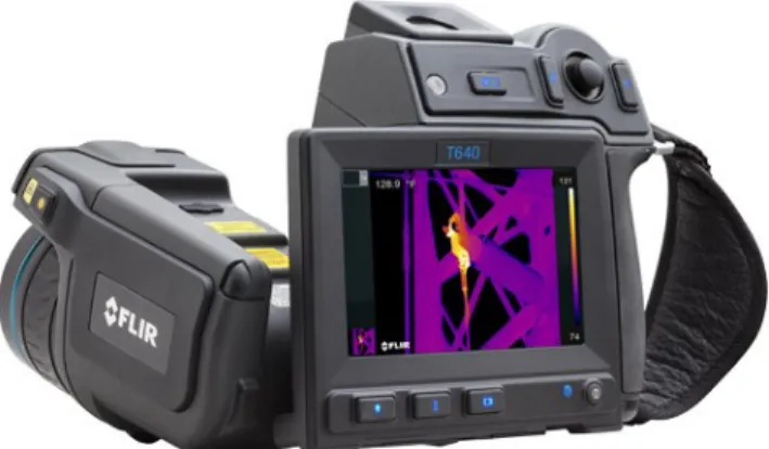
The last piece of equipment is the FLIR T640 Infrared Thermographer, shown in Figure 3-3. It was chosen for its broad temperature range and accuracy. It can detect temperatures in the range of -40oF to 3632oF with an accuracy of 2% or 3.6oF, whichever is larger. Once the thermal images have been collected, the FLIRTools+ software can be used for post-processing the data (FLIR T-Series).
27
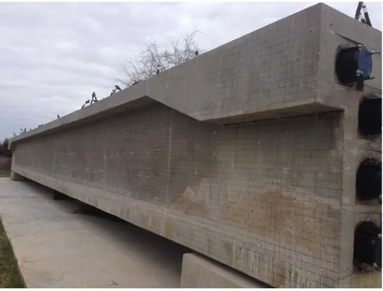
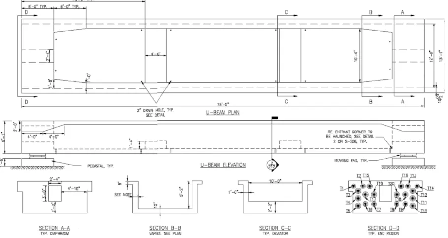
3.3Test Specimen
In order to test the effectiveness of the NDT methods, a 75-ft (22.86-m) long U-shaped bridge girder was constructed. A photograph of the constructed bridge girder appears in Figure 3-4, and the detailed construction drawings appear in Figure 3-5. The girder is 13 ft 9 in. wide and 6 ft 1 in. tall from the base of the slab to the top of the flange. The walls are typically 12 in. thick and the flanges overhang the outside walls by 10.5 in. The anchorage zones at each end are 6 ft long and contain standard sized access holes measuring 3 ft high by 2 ft 4 in. wide. The deviators are 10 ft wide, 4 ft long, and 16 in. high. The girder is simply-supported at its ends by two pedestals, each measuring 1 ft 6 in. above the work slab. Bearing pads are utilized between the pedestals and the girder.
28
29
Twenty PT ducts were utilized and are distributed as follows: six are external, four are located in the slab, two are located in each flange, and three are located in each girder wall. The external ducts and those in the walls of the specimen each contain 19 PT strands. The ducts in the slab and flange each consist of twelve PT strands. Each strand is 0.6 in. (15.24 mm) in diameter and consists of seven wires. The concrete cover for the internal ducts in the girder web is approximately 4 in., although it varies near the anchorage zones.
To test the effect of duct material on the NDT methods, both metal and high-density polyethylene (HDPE) ducts were utilized. The external tendons (T15, T16, T17, T18, T19, and T20) all have smooth 4-in. HDPE ducts with metal duct sections inside the deviator and anchorage regions. Conversely, corrugated ducts were utilized for all internal tendons, although they vary in material and size. The internal tendons on the North side of the specimen consist of metal ducts, while the tendons on the South side of the specimen have HDPE ducts. The duct specifications by tendon are detailed in Table 3-1.
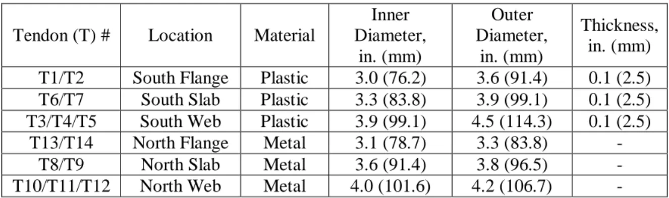
Table 3-1: Internal Duct Specification by Tendon
Tendon (T) # Location Material
Inner Diameter, in. (mm) Outer Diameter, in. (mm) Thickness, in. (mm) T1/T2 South Flange Plastic 3.0 (76.2) 3.6 (91.4) 0.1 (2.5) T6/T7 South Slab Plastic 3.3 (83.8) 3.9 (99.1) 0.1 (2.5) T3/T4/T5 South Web Plastic 3.9 (99.1) 4.5 (114.3) 0.1 (2.5)
T13/T14 North Flange Metal 3.1 (78.7) 3.3 (83.8) -
T8/T9 North Slab Metal 3.6 (91.4) 3.8 (96.5) -
30
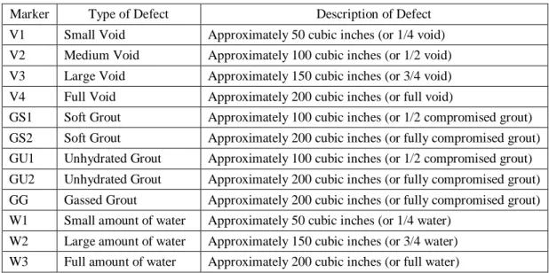
A complex defect design was developed and implemented. The defects include grout voids and water filled cavities of varying sizes, as well as several grout conditions, including soft grout, unhydrated grout, and gassed grout. Table 3-2 details each grout defect and gives its identifying marker.
Table 3-2: Grout Defect Marker and Description
Marker Type of Defect Description of Defect
V1 Small Void Approximately 50 cubic inches (or 1/4 void)
V2 Medium Void Approximately 100 cubic inches (or 1/2 void)
V3 Large Void Approximately 150 cubic inches (or 3/4 void)
V4 Full Void Approximately 200 cubic inches (or full void)
GS1 Soft Grout Approximately 100 cubic inches (or 1/2 compromised grout)
GS2 Soft Grout Approximately 200 cubic inches (or fully compromised grout)
GU1 Unhydrated Grout Approximately 100 cubic inches (or 1/2 compromised grout) GU2 Unhydrated Grout Approximately 200 cubic inches (or fully compromised grout) GG Gassed Grout Approximately 200 cubic inches (or fully compromised grout) W1 Small amount of water Approximately 50 cubic inches (or 1/4 water)
W2 Large amount of water Approximately 150 cubic inches (or 3/4 water) W3 Full amount of water Approximately 200 cubic inches (or full water)
In addition to grout defects, various amounts of corrosion and section loss were also included for future research. These defects are detailed in Table A-1 of Appendix A. The defect keys in Figure 3-6 show the types and location of defects for all internal tendons. Note that no defects were included in the slab tendons T6, T7, T8, and T9.
31
(a) North Wall: Tendons T10, T11, T12
(b) South Wall: Tendons T3, T4, T5
(c) Flange (plan view): Tendons T1, T2, T13, T14
32
CHAPTER IV
ULTRASONIC TOMOGRAPHY
4.1Introduction
Ultrasonic waves are reflected at material interfaces due to a change in acoustic impedance. Consequently, ultrasonic tomography (UST) was utilized in an effort to identify grout defects in the internal ducts of the 75-foot post-tensioned bridge girder.
4.2Procedure
A 1.97 x 1.97 in. (50 mm x 50 mm) grid system was applied to all regions of the bridge girder which were to be scanned. This included both the internal and external sides of the bridge girder walls, the flanges, and the deviators. When scanning, a horizontal step of 5.91 in. (150 mm) and a vertical step of 1.97 in. (50 mm) were utilized. The operational frequency was set to 50 kHz, and the specimen was scanned with the device oriented both parallel and perpendicular to the ducts. Because of the size of the specimen and the limited internal storage of the MIRA device, the data was
collected in sections and combined afterward. Concrete is a nonhomogeneous material, so to properly estimate the velocity of the shear wave emitted by the MIRA transducers, sample velocities were obtained and averaged for each section of the specimen. These velocities are documented in Table A-2 of Appendix A.
33
4.3Girder Wall Results
The results are presented for each wall, along with the corresponding defect keys. The depths of the presented scans are detailed in each caption. It is important to note that the regions shown in black were not accessible. This could be due to the physical limitations of the device and/or the design of the bridge specimen.
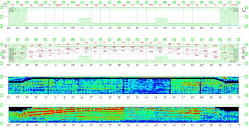
Figure 4-1 and Figure 4-2 present the results from testing the North Wall of the bridge girder. The metal ducts themselves are difficult to identify, particularly when the device was oriented parallel to the ducts, as in Figure 4-1c and Figure 4-2c. This is consistent with previous research which suggests that thin walled metal ducts are transparent to incident acoustic waves. However, from these figures, it appears as though the A1040 MIRA is unable to consistently identify any grout defects. In Figure 4-1c and Figure 4-1d, higher reflections are observed between markers S (54 ft) and V (63 ft), suggesting that the MIRA could possibly identify sizeable water defects; however, further exploration is needed before this can be concluded definitively.
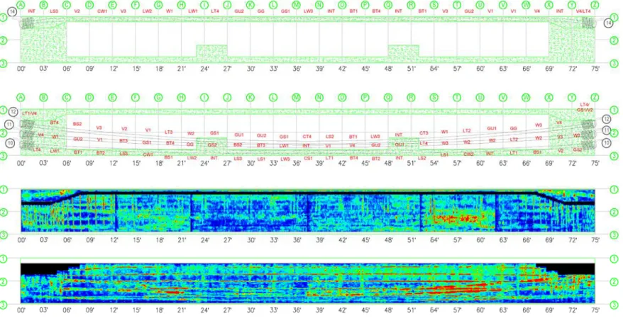
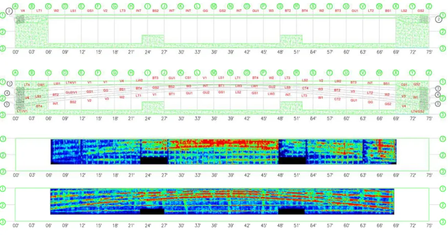
The results from testing the South Wall of the bridge girder appear in Figure 4-3 and Figure 4-4. The device was quite successful in identifying the HDPE plastic ducts when the device was oriented perpendicular to the ducts as in Figure 3d and Figure 4-4d. However, the large reflections caused by the plastic ducts make the grout defects unidentifiable using this method.
It should be noted that the external walls were scanned using six sections, and the internal walls were scanned using seven sections. In images where the device was oriented parallel to the ducts, such as Figure 4-1c, the division of these sections is clearly
34
apparent, as they are marked by small vertical blue regions. These regions correspond to areas with less information. With a horizontal step of 5.91 in. (150 mm), each scan overlaps the previous by 8.86 in. (225 mm). These blue regions correspond to the beginning of each new section and consequently to areas where there is no overlap in the data. Even in scans when the device was oriented perpendicular to the ducts, i.e. Figure 4-2d, some of the section divisions are also visible. This could be due to a number of factors, including but not limited to the change in velocity from section to section or possibly inconsistent pressure, as multiple individuals were used to scan the specimen.
35 (a)
(b)
(c)
(d)
Figure 4-1: North Wall Exterior Scans – MIRA: (a) Tendon 14 Defect Key; (b) North Wall Defect Key; (c) MIRA Device Parallel to Ducts (Wall Scan Depth: 2.88 – 9.66 in.; Flange Scan Depth: 6.51 – 9.66 in.); (d) MIRA Device Perpendicular to Ducts (Wall Scan Depth: 2.88 – 9.66 in.)
36 (a)
(b)
(c)
(d)
Figure 4-2: North Wall Interior Scans – MIRA: (a) Tendon 13 Defect Key; (b) North Wall Defect Key; (c) MIRA Device Parallel to Ducts (Scan Depth: 2.88 – 9.66 in.); (d) MIRA Device Perpendicular to Ducts (Scan Depth: 2.88 – 9.66 in.)
37 (a)
(b)
(c)
(d)
Figure 4-3: South Wall Exterior Scans – MIRA: (a) Tendon 1 Defect Key; (b) South Wall Defect Key; (c) MIRA Device Parallel to Ducts (Wall Scan Depth: 2.88 – 9.66 in.; Flange Scan Depth: 6.51 – 8.77 in.); (d) MIRA Device Perpendicular to Ducts (Wall Scan Depth: 2.88 – 9.66 in.)
38 (a)
(b)
(c)
(d)
Figure 4-4:South Wall Interior Scans – MIRA: (a) Tendon 2 Defect Key; (b) South Wall Defect Key; (c) MIRA Device Parallel to Ducts (Scan Depth: 4.04 – 9.66 in.); (d) MIRA Device Perpendicular to Ducts (Scan Depth: 2.88 – 9.66 in.)
39
4.4Deviator Results
The deviators were also scanned using the A1040 MIRA ultrasonic tomographer. While the ducts are identifiable, again the grout defects are not distinguishable from good grout. The images in Figure 4-6, when the device is oriented perpendicular to the ducts do have better resolution than the images in Figure 4-5, when the device is oriented parallel to the ducts. This is consistent with the results of the wall scans.
(a)
Dev. 1 Defect Key
(b) Dev. 1 Scan
(c)
Dev. 2 Defect Key
(d) Dev. 2 Scan
Figure 4-5:Deviator Scans – MIRA Device Oriented Parallel to Ducts (Dev 1 Scan Depth: 5.82 – 12.33 in.; Dev 2 Scan Depth: 5.82 – 12.33 in.)
40 (a)
Dev. 1 Defect Key
(b) Dev. 1 Scan
(c)
Dev. 2 Defect Key
(d) Dev. 2 Scan
Figure 4-6:Deviator Scans – MIRA Device Oriented Perpendicular to Ducts (Dev 1 Scan Depth: 5.82 – 12.33 in.; Dev 2 Scan Depth: 6.17 – 11.85 in.)
4.5Summary
Implementing the ultrasonic technique took approximately 278 hours. This includes applying the grid system, scanning the specimen, and processing the collected data. Applying the grid to the specimen took approximately 116 hours. The scanning and processing times for each orientation are detailed in Table 4-1.
41
Table 4-1: UST Scanning & Processing Times
UST Parallel UST Perpendicular Location Scanning Time (hours) Processing Time (hours) Scanning Time (hours) Processing Time (hours) North Wall Exterior (including Flange) 17.00 4.0 13.25 3.25
North Wall Interior 17.50 4.0 11.75 3.25
South Wall Exterior (including Flange) 19.00 4.0 11.50 3.25
South Wall Interior 17.00 4.0 11.00 3.25
Deviator 1 2.50 1.0 2.50 1.25
Deviator 2 2.50 1.0 2.50 1.25
In analyzing the processed data, it was discovered that the MIRA A1040
ultrasonic tomographer should be oriented perpendicular to the ducts for the best results. This orientation provides better quality images with higher resolution. The equipment was quite successful in identifying the HDPE plastic ducts. However, the large
reflections caused by the plastic ducts prevent the identification of grout defects. Conversely, the thin walled metal ducts appear transparent to the incident acoustic wave and produce little to no reflection. Consequently, the MIRA A1040 ultrasonic
tomographer may be able to identify sizeable water defects. Further studies to test this hypothesis are required. Other forms of grout defects, including unhydrated grout, gassed grout, soft grout, and voids were not identifiable, regardless of the size of the defect.
42
CHAPTER V
GROUND PENETRATING RADAR
5.1Introduction
High frequency radio waves are reflected at material interfaces due to a change in the dielectric properties. The size of this contrast determines the strength of the reflected wave. Consequently, ground penetrating radar (GPR) seems ideal for identifying grout defects in internal ducts of post-tensioned bridge girders.
5.2Procedure
The same grid system that was applied to the specimen for the ultrasonic
tomography testing is utilized for the GPR testing. Because of the size of the specimen, it was divided into several sections. Each line, both vertical and horizontal, was scanned and later combined in the RADAN software. A dielectric constant of 9 and a scan depth of 16 in. (406.4 mm) were selected.
5.3Girder Wall Results
The results are presented for each wall, along with the corresponding defect keys. It should be noted that the depth of each scan is provided in the figure captions and that each wall scan has a thickness of 3.54 in. (90 mm). Also note that any white or gray areas in the images were inaccessible. This could be due to the physical limitations of the device and/or the design of the bridge specimen.
43
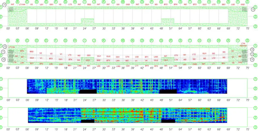
Figure 5-1 presents the GPR results for the North Wall. The metal ducts are clearly identifiable in both the interior and exterior wall scans, as they produce strong reflections. However, these reflections prevent the grout defects from being identified. These results are consistent with those observed by other researchers as detailed in Chapter II.
The South Wall results in Figure 5-2. The plastic ducts do not provide as strong reflections, making them more difficult to identify. This is especially true in the interior wall scan. While in theory this would allow for the grout defects to be better observed, they are not discernable in these images. This could partially be attributed to the orientation of the voids as reported by other researchers (Pollock et al., 2008).
44 (a)
(b)
(c)
(d)
Figure 5-1:North Wall Scans – GPR: (a) Flange Defect Key (Plan View); (b) North Wall Defect Key; (c) Exterior Wall Scan (Wall Scan Depth: 4.58 in.; Flange Scan Depth: 6.46 in.); (d) Interior Wall Scan (Scan Depth: 5.41 in.)
45 (a)
(b)
(c)
(d)
Figure 5-2: South Wall Scans – GPR: (a) Flange Defect Key (Plan View); (b) South Wall Defect Key; (c) Exterior Wall Scan (Wall Scan Depth: 4.78 in.; Flange Scan Depth: 6.08 in.); (d) Interior Wall Scan (Wall Scan Depth: 5.36 in.)
46
5.4Deviator Results
The deviator results appear in Figure 5-3 and are consistent with the wall data. The metal ducts within the deviators are clearly identifiable, but the defects themselves are not. It should be noted that the deviator scans are 1.77 in. (45 mm) thick and that the gray regions in Figure 5-3d were inaccessible due to the external tendons T15 and T16, which pass over the deviator rather than through it.
(a)
Dev. 1 Defect Key
(b) Dev. 1 Scan
(c)
Dev. 2 Defect Key
(d) Dev. 2 Scan
Figure 5-3:Deviator Scans – GPR
(Dev 1 Scan Depth: 4.44 in.; Dev 2 Scan Depth: 4.44 in.)
5.5Summary
Implementing the GPR technique took approximately 191 hours. This includes applying the grid system, scanning the specimen, and processing the data. The grid system which was applied for the ultrasonic method was utilized for the GPR testing.
47
The application of this grid took approximately 116 hours. The scanning and processing times are detailed in Table 5-1.
Table 5-1: GPR Scanning & Processing Times
GPR Location Scanning Time (hours) Processing Time (hours) North Wall Exterior (including Flange) 12.25 5.0
North Wall Interior 8.00 8.0
South Wall Exterior (including Flange) 13.75 5.0
South Wall Interior 8.75 8.0
Deviator 1 1.0 2.0
Deviator 2 1.0 2.0
The collected data revealed the capabilities and limitations of the GPR method. It is highly effective at locating embedded steel ducts, but it cannot locate grout defects due to the strong observed reflections. It is able to identify the plastic ducts, but
provided no information about the condition of the grouted tendons. This is possibly due to the size and orientation of the voids.
48
CHAPTER VI
INFRARED THERMOGRAPHY
6.1Introduction
Various materials absorb and release heat at different rates. Therefore, the uneven cooling or heating of the specimen due to the metal or HDPE plastic ducts, the surrounding concrete, the good grout, and the various defects, should be identifiable in a temperature profile. Infrared thermography (IRT) was thus chosen in an attempt to identify the various grout defects. Solar energy was chosen as the heat source due to the size of the specimen.
6.2Procedure
Williams’s (2014) research suggests that the IRT technique be applied when the ambient temperature is changing rapidly. This is when the method is most effective. Consequently, a temperature study of previous years was conducted to determine the most appropriate time to utilize this method. Figures of the collected data appear in Appendix B. The temperature study revealed that the images should be taken between the hours of 8:00 – 11:00 am and/or 4:30 – 7:30 pm. All infrared images were taken during these time frames. Experimentation proved that the evening pictures not only created safety concerns, as the sun set around 6:00 pm, but were also less useful, as the specimen took an immense time to cool.
49
Because of the size of the specimen, the angle of the camera lens, and physical limitations, eight images were required to capture the full length of each external wall, and twenty-one images were required to capture the full length of each interior wall. These photos were taken using a single temperature scale and later stitched together to produce one full length image. The walls were photographed numerous times in an effort to capture the uneven cooling/heating. Each round of images was taken
approximately 10 – 15 minutes apart. To maintain consistency, tripod locations were selected and marked along the perimeter of the specimen. Both the girder walls and the end caps were photographed.
6.3Results
The images of the North Wall are presented in Figure 6-1 and Figure 6-2, while Figure 6-3 and Figure 6-4 present the results from the South Wall. The East End Cap images are shown in Figure 5 and Figure 6. The West End Caps appear in Figure 6-7. A temperature scale for each image is provided.
6.3.1North Wall Results
The angled images of the North Wall in Figure 6-1 do not reveal any information about the ducts or the grout defects. However, from these images the surface condition can be assessed, as the uneven, grinded surfaces near the ends of the specimen and above the bottom slab are visible. These are simply features from the construction process.
50
(a) Photographed from the NE
(b) Photographed from the NW
Figure 6-1:North Wall Exterior IRT Image
The defect key for the North Wall appears in Figure 6-2, along with images of the interior and exterior. While the rough anchorage zones and slab line are again
51
visible, the metal ducts are not. In Figure 6-2c, a small warm rectangle appears on the flange near marker X (69 ft). This is actually a 2 in. x 4 in. piece of lumber used in the formwork that remains in the specimen. The piece of wood cools at a different rate than the surrounding concrete and so it is visible in the temperature profile.
It should be noted that Figure 6-2d shows a fairly large temperature differential between the two ends of the wall. In the morning, the interior west side of the North Wall receives direct sunlight while the east side is shaded. While ideally, the entire specimen should be shaded or in direct sunlight, the orientation of the specimen did not provide such an opportunity. This point becomes moot as the technology does not appear to be able to locate the internal ducts or their defects. Please note that an external duct is visible in this image due to its proximity to the internal wall.
52 (a)
(b)
(c)
(d)
Figure 6-2:North Wall Images – IRT: (a) Flange Defect Key (Plan View); (b) North Wall Defect Key; (c) Exterior Wall Image; (d) Interior Wall Image
53
6.3.2South Wall Results
The HDPE plastic ducts are not visible in the angled images of the South Wall in Figure 6-3. The rough anchorage zones and slab line are visible. There are two
anomalies in these images which are quite interesting. The anchorage zones appear to be comparatively warmer than the rest of the specimen. Warmer regions also appear along the wall surface on each side of center. A full length IRT image of the girder wall will likely provide further information and perhaps offer an explanation for these abnormally warm regions.
54
(a) Photographed from the SE
(b) Photographed from the SW
Figure 6-3:South Wall Exterior IRT Image
The South Wall defect key, as well as the full length infrared images, is presented in Figure 6-4. From this figure, it is apparent that the anchorage zones are
55
indeed warmer than the surrounding areas. The two warmer spots on either side of center, which were identified in Figure 6-3, are clearly visible and correspond to the deviator regions. It is possible that these regions are warmer due to the additional wall thickness. Due to the proximity of the external ducts to the interior walls, an external tendon is visible in Figure 6-4d. However, no internal ducts or grout defects are visible.
It is likely that the ducts are embedded too far into the wall to be visible using infrared thermography. These results are consistent with previous research. Musgrove (2006) discovered that a temperature gradient of at least 135ºF (75ºC) is required in order to detect simulated voids with concrete covers of 2 in. (50.8 mm) or less, and Pollock et al. (2008) noted the difficulty in obtaining the necessary temperature gradient in thicker concrete specimens, particularly when the heat can propagate along the length and height of a specimen. An exploration of the end cap regions should provide more promising results.
56 (a)
(b)
(c)
(d)
Figure 6-4:South Wall Images – IRT: (a) Flange Defect Key (Plan View); (b) South Wall Defect Key; (c) Exterior Wall Image; (d) Interior Wall Image
57
6.3.3East End Cap Results
From Figure 6-5 and Figure 6-6, it is apparent that the grout condition of the end cap regions is not consistent. By compiling data from each of the images, it appears as though tendons T4, T11, T12, T17, T18, T19, and T20 have large grout defects, as they appear much warmer than the other end caps. This might be expected if they are not completely grouted, but rather completely voided or filled with water. Tendon T5 appears to have a much smaller defect, as there is a distinct line across the end cap suggesting a material change. That is, the end cap appears to be mostly grouted, but also contain a slight void or small water-filled cavity.
After comparing with the defect key, these hypotheses are determined to be correct. However, not visible in these figures is the complete void in tendon T2. The end cap for tendon T2 appears to be pointed down and away from the eastern morning light. Thus, it does not heat up like the other end caps with voids.
58
(a) East End Cap Defect Key
(b) East End Cap Image - IRT
(c) East End Cap Image - IRT
59
(a) East End Cap Defect Key
(b) East End Cap Image - IRT
Figure 6-6: East End Cap Images – IRT
60
6.3.4West End Cap Results
From Figure 6-7, it appears as though tendons T1, T14, and T18 are completely ungrouted at the anchorage zone, while tendons T11, T12, T15, T16, T17, T19, and T20 are partially ungrouted. These regions are likely to be voided or contain water-filled cavities. After comparing with the defect key, these hypotheses are deemed to be correct. However, the small water defect in tendon T4 is not identifiable. Additionally, the IRT camera does not appear to be able to distinguish between the water-filled
cavities and voids or between “good grout” and soft grout. However, it seems extremely reliable in determining whether a duct’s cross-section is fully grouted or if a water/void defect is present.