Transition Detection at Cryogenic Temperatures Using a
Carbon-Based Resistive Heating Layer Coupled with
Temperature Sensitive Paint
A. Neal Watkins,1 Kyle Z. Goodman,2 and Sarah M. Peak3NASA Langley Research Center, Hampton, VA, 23681
This paper will highlight the development and application of a carbon-based resistive heating layer for use in transition detection at cryogenic temperatures at the National Transonic Facility (NTF) for full-flight Reynolds number testing. This study builds upon previous work that was successfully demonstrated at the 0.3-m Transonic Cryogenic Tunnel on a smaller-scale airfoil shape of regular geometry. However, the test performed at the NTF involved a semispan wing with complex geometry and significantly larger than previous tests. This required the development of new coatings to provide suitable resistances to provide adequate heating rates for transition detection. Successful implementation of this technology has the ability to greatly enhance transition detection experiments at cryogenic temperatures as well as reducing perturbation in the tunnel caused by more traditional transition detection methods.
I.
Introduction
For the validation of aerospace vehicle concepts and prediction tools, it is often desired to test in conditions that most closely resemble those of flight. This is generally performed in a high Reynolds number environment, in which the momentum of the fluid dominates the flow, and turbulent flow is present. High Reynolds number ground-based testing of aerospace models and concepts is often undertaken in facilities capable of operating at cryogenic conditions, in which cooling the test gas to near liquid nitrogen temperatures can achieve Reynolds numbers approaching 500 M/m. [1] One important aspect that is often desired in this type of testing is the knowledge of where the flow transitions on the surface from laminar to turbulent. The determination of this location can be critical for accurate drag estimation, and there are efforts underway to design wing shapes and vehicle concepts that can delay this transition for drag reduction (leading to decreased fuel usage). The location of transition is typically indicated by the change in the adiabatic wall temperature on the surface in areas of laminar versus turbulent flow.
There are several methods to determine transition location in ambient facilities, including multi-element hot-film sensor systems [2-4], sublimating chemicals, [5-6], and infrared (IR) thermography [7-9]. The multi-element hot-film sensors have been demonstrated down to cryogenic conditions [10]. However, these are point-based measurements that have difficulty providing global measurements on complex models. Both sublimating chemicals and IR thermography can provide these global measurements, but each suffers from distinct disadvantages operating in a cryogenic facility. Sublimating chemicals require frequent access to the model, and to date there are no chemicals that can be applied for cryogenic testing that will not sublimate immediately at ambient conditions. IR thermography can directly image these temperature changes, and measurements at cryogenic conditions have been accomplished using a commercially available IR camera in the 8-12 µm wavelength range [11] and using a specially designed long-wave IR camera (13-15 µm wavelength range) capable of operating at -173 oC [12]. However, standard IR thermography suffers from the inherent low amount of IR radiation present at cryogenic conditions, and the custom camera provided relatively small image sizes (128 x 192 pixels) and requires liquid helium cooling of the sensor for operation.
An alternative to these techniques for detecting transition at cryogenic temperatures is based on Temperature Sensitive Paint (TSP) [13-15]. TSP is typically composed of a gas impermeable binder in which a luminescent molecule is immobilized. [16] With a suitable binder, changes in the output of the luminescent molecule are due to the changes in the quantum yield due to changes in temperature (i.e. thermal quenching). The relationship between
1 Aerospace Technologist, Advanced Measurements and Data Systems Branch, Mail Stop 493, Senior Member AIAA. 2 Research Scientist, Advanced Measurements and Data Systems Branch, Mail Stop 493.
3 Research Scientist, Advanced Measurements and Data Systems Branch, Mail Stop 493.
the luminescence of the probe molecule and the absolute temperature generally follows Arrhenius behavior over a certain range [16] REF NR REF R T T E T I T I 1 1 ) ( ) ( ln (1)
where ENR is the activation energy for the non-radiative process, R is the universal gas constant, and TREF is the reference temperature. However, for some TSPs, Eq. (1) cannot fully describe the behavior, especially outside of temperature ranges where Arrhenius behavior occurs. Thus, it is also common to simply model the behavior of the TSP in a more generalized sense
) / ( ) ( / ) (T I TREF f T TREF I (2)
where f(T/TREF) is a function that can be linear, polynomial, exponential, etc., to fit the experimental data over a
suitable temperature range. This behavior is dependent on the nature of the probe, thus it is possible to select molecules that can lead to formulations that are temperature sensitive from cryogenic to 200 oC [13-15, 17,18].
Traditionally, for detecting transition at cryogenic conditions, a temperature step is introduced into the tunnel to enhance the natural temperature change due to transition (depending on flow temperature and local Mach number, this can be on the order of 0.1 oC or less). This is usually accomplished by rapidly changing the liquid nitrogen injection rate into the tunnel in either a positive (less nitrogen flow, resulting in a temperature ramp up) or a negative (more nitrogen flow, resulting in a temperature ramp down) direction. While quite effective in increasing the temperature experienced on the model, this can add a significant cost in terms of data acquisition time and facility operation. In addition, there can also be a significant change in the local flow conditions during the step.
Recently, however, work has been presented combining TSP with a carbon-based heating layer. [19-21]The heating layer acts as a resistive heater that can locally increase the temperature on the model surface when current is flowed through it. This provides a means to apply a temperature step directly to the model (as opposed to the flow), greatly decreasing the data acquisition time (as the tunnel does not need to recover after each temperature step) and stability in the flow conditions. Optimization of the technique has allowed demonstrations down to -163 oC on smaller airfoil shapes.
This work seeks to expand previous efforts and deploy this technology on a much larger scale. For this effort, a NASA Common Research Model with Natural Laminar Flow (CRM-NLF) was chosen. Not only was the area to be heated much larger (>1000 in2 vs. ~96 in2 for the airfoil), but the aspect ratio between the inboard region and the tip region was significantly different. This work will present results from this test including a description of the coatings employed. A full analysis of these results in regards to the aerodynamic implications can be found in Lynde, et. al. [22]
II.
Materials and Methods
A. Wind Tunnel Facility
This testing was carried out at the National Transonic Facility (NTF) at NASA Langley research Center. The NTF is a unique facility [23] that can provide high quality flight Reynolds number aeronautical data. The tunnel has a test section of 2.5 meters x 2.5 meters and is capable of operating at speeds from subsonic (M = 0.1) to transonic (M = 1.1) with Reynolds numbers from 13.1 x 10⁶/m to 476 x 106/m. While standard operation of the tunnel is performed using air as a test gas, the tunnel is also capable of operating at cryogenic conditions (down to -156 oC) by injecting liquid nitrogen into the tunnel circuit. In the cryogenic operating mode, the NTF is capable of providing full-scale flight Reynolds numbers without an increase in model size. Since the 1990s, the tunnel has mounting support and can test either full-span (typically sting-mounted) or semi-span models (mounted to the side-wall).
B. Model Description
The CRM-NLF model used in this testing is a semi-span wing and is a combination of a new NLF semispan wing and existing 5.2% Boeing 777 semispan hardware. The new wing was designed by Campbell and Lynde [24] and fabricated by Advanced Technologies, Inc. The new wing mounts to the existing 777 hardware with new fairings that were manufactured because the outer mold line of the new wing is different than the 777 wing at the wing-fuselage
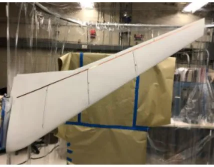
juncture. The wing mounted in the NTF is shown in Fig. 1. More details of the wing and testing philosophies can be found in Rivers et al. [24]
C. Carbon-based Heating Layer
Due to the relatively low resistance of the previous carbon-based heating layer [21], new formulations were developed to try and tailor the resistance so that the maximum power could be applied safely to the model surface. These formulations were based on the same polyurethane binder that the TSP is based on. However, instead of adding the TSP dye, the suitable carbon-based material was added. For this work, two different carbon-based materials were selected; carbon black and graphite. These materials exhibit relatively high conductivity and have been used previously in resistive heating applications. [26-28] The general method to make each formulation was to measure the appropriate pigment (either carbon black or graphite) amount and disperse it in a suitable solvent. This was then added to the polyurethane binder and applied using traditional airbrushing techniques. For the carbon black formulations, it was found that the pigment could be dispersed in toluene. However, when graphite is used as the pigment, it was found that xylene was required as the flashpoint of toluene was too
low so that the graphite-based films typically cracked. If higher concentrations of graphite are needed, it was generally found that the addition of small amounts of N-methyl-2-pyrrolidone (NMP) allowed for the creation of better films. The general components of each formulation is shown in Table 1.
Table 1. Composition of carbon-based heating layer formulations
Pigment Concentration (based on binder) Solvent System
Carbon Black 25% Toluene
Graphite 25% Xylene
Graphite 75% Xylene:NMP (80:20 v/v)
For this work, the final overall resistance of the carbon black-based system was typically 130-250 Ω, while that of the graphite-based system was typically 60-100 Ω. It should also be noted that this is dependent on many factors, including but not limited to: thickness of the heating layer, area, aspect ratio, etc.
D. TSP
For this test, the requested temperature range is from -100 oC to 40 oC, which is a greater range than most typical TSP formulations are sensitive. As such, an alternative formulation containing two different ruthenium dyes was developed. The overall formulation was based on those developed at NASA LaRC and have been used for transition detection at cryogenic conditions at the NTF [29] and for measurement of heating properties at hypersonic conditions. [30] For this work, the two dyes chosen were ruthenium terpyridine
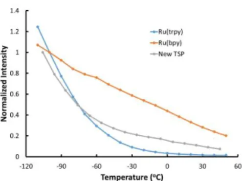
(Ru(trp)) and ruthenium bipyridine (Ru(bpy). The Ru(trp) dye is what is traditionally used in cryogenic testing, and shows excellent temperature sensitivity down to < -150 oC. However, the luminescence of the dye is highly quenched at ambient temperatures. To account for this, Ru(bpy) was selected, as it is traditionally used for temperature measurements at ambient conditions. This combination of dyes was selected mainly for the ease of integration with the existing instrumentation. Egami, Fay, and Quest demonstrated a TSP system capable of these temperature ranges by mixing multiple dyes. [31] However, it also required the use of separate excitation wavelengths depending on the temperature range in question. On the other hand, the mixture described here uses the same excitation and emission wavelengths. This is very important in the NTF facility as optical access is extremely limited. A typical response curve for the formulation is shown in Fig. 2. While the
Fig. 1. CRM-NLF wing mounted in the NTF.
Fig. 2. Response curve of new TSP compared with standard Ru(trpy) and Ru(bpy) TSPs
luminescent output is lower at ambient conditions, it is at least a factor of ten greater than just relying on Ru(trpy) alone. The amount of Ru(bpy) added was based on being able to achieve the largest signal increase at ambient temperatures while maintaining the higher sensitivity at cryogenic conditions.
E. Preparation of the TSP/Heating Layer System
The TSP/heating layer system consisted of several layers which are illustrated in Fig. 3. These layers are labelled in Fig. 3 and described below. First, an adhesion layer (1) was applied to the surface and allowed to cure in air. Next, a white polyurethane layer (2) was applied to act as an electrical insulation layer. This layer can be either air cured overnight or cured at 70 oC for 2 hours. After this layer is cured, the electrical connections (C) are applied. For this work, simple copper tape was employed. Then the
carbon-based polyurethane heating layer (3) was applied and allowed to cure in air overnight. Next, another layer of the white polyurethane was applied (4). This layer is needed as the heating layer is black in color. The white layer serves to scatter more of the emission light away from the surface for collection by the camera. Finally, the TSP topcoat (5) was applied and allowed to air cure. In this work, a thicker layer of TSP was applied to mitigate the possibility of leading edge damage. With a suitable thickness of TSP, the layer could be polished as needed without removing the entire TSP layer.
One of the requirements for a successful natural laminar flow test is that the surface must be extremely smooth so that the very thin boundary layers are not tripped by paint edges, roughness spots, etc. By using a TSP made from a harder polyurethane layer, the upper surface could be worked to a very smooth finish. Briefly this was done by first lightly wet-sanding with 1500-grit sandpaper to remove imperfections, blemishes, and debris that landed on the model. Once this is done, a random orbital polisher was used with gradually increasing orbit speed to produce a mirrored finish with typical roughness (Ra) on the order of 0.02 µm or better. This was typically measured at 50% chord. Measurements on the leading edge were more difficult to obtain with the equipment available, but these were typically on the order of 0.04 µm.
Current is applied to the carbon-based layer using thin copper tape strips as described above. These strips are placed directly on the electrically insulating layer prior to the application of the polyurethane layer with the carbon pigment. For this work, it was desired to keep the leading edge free of steps, which would be caused if the tape conductors were placed chordwise on the wing. Therefore, the copper tape strips were placed spanwise, with one strip placed on the upper surface and one placed on the lower surface. The placement of the strip on the upper surface is shown in Fig. 4. The copper strip on the lower surface was placed much closer to the leading edge. This greatly reduced the amount of area to be heated that would not be imaged.
F. Instrumentation
Illumination of the TSP layer was accomplished using custom light emitting diode (LED) arrays built to withstand the temperatures and pressures experienced in the NTF. The
LEDs emit at 400 nm (20 nm bandwidth at full width at half maximum). The LEDs were also equipped with a short pass optical filter to remove the red tail that is present in the output of the lamps.
Image acquisition was accomplished using a pair of 11 megapixel cameras (Imperx 11M5) equipped with a long pass filter to acquire the TSP signal. The cameras were interfaced with the computer via a fiber optic interface, and acquisition was triggered by the tunnel data systems.
Powering of the heating layer was accomplished using various programmable laboratory power supplies. For the first portion of the test, a single power supply capable of applying up to 600V at up to 2.6A (1560W). The overall resistance of
Fig. 3. Schematic of TSP/heating system layer. Components are; 1. Adhesion layer; 2. Polyurethane electrically insulating layer; 3. Carbon-based polyurethane layer; 4. White polyurethane layer; 5. TSP layer; C. Copper tape electrodes.
Fig. 4. Copper tape electrode placed near trailing edge on the upper surface of the CRM-NLF.
the coating system determined the maximum amount of power that could be applied and for this portion of the test, ~900W was power was applied. For the second portion of the test, a second identical power supply was employed, and the power supplied were placed in parallel. Thus the available power was 3120W. For this portion of the test, power up to ~2000W was applied.
G. Data Acquisition
In order to use TSP for transition visualization, it is often necessary to use an image that does not have a heating step applied to use a reference. This is typically done by taking an image (or set of images for averaging) before the temperature step is applied and then forming a ratio of the two images. For the more traditional temperature step runs, this is fairly simple as it takes a finite amount of time before the temperature step induced by nitrogen flow reaches the model. In this test, it was generally about 5 seconds. For these temperature step runs, the data acquisition procedures was:
1) Establish the proper flow conditions with the model in the correct position. 2) Initiate the tunnel data acquisition. This also starts the cameras acquiring images. 3) Initiate the temperature step by altering the nitrogen injection system.
4) Acquire tunnel (and image) data for 30 seconds. 5) Move the model to the next position.
6) Wait for the tunnel to recover to the correct flow conditions. 7) Collect the next point.
For these sets of data, the first several images can be used as the reference image as no temperature change is occurring. Therefore, the required ratio is calculated by simply dividing each image collected during the data point by the reference image chosen in the same data point.
For the heating layer runs, it was found that the most efficient way to acquire this data was to acquire a pair of polars. The first polar was with the heating layer unpowered and was used as the reference images. The second polar was acquired with the heating layer on. For these runs, the data acquisition procedure was:
1) Acquire a polar with the desired angle of attack values. For each angle of attack, images are acquired as triggered by the wind tunnel data acquisition system.
2) Return the model to the polar starting point.
3) Energize the heating layer and allow the layer to “pre-heat.” This typically required about 2 minutes. 4) Re-run the polar with the heating layer on.
5) Return the model to the original position, de-energize the heating layer and prepare for the next condition.
III. Results and Discussion
A. Carbon Black-Based Heating Layer
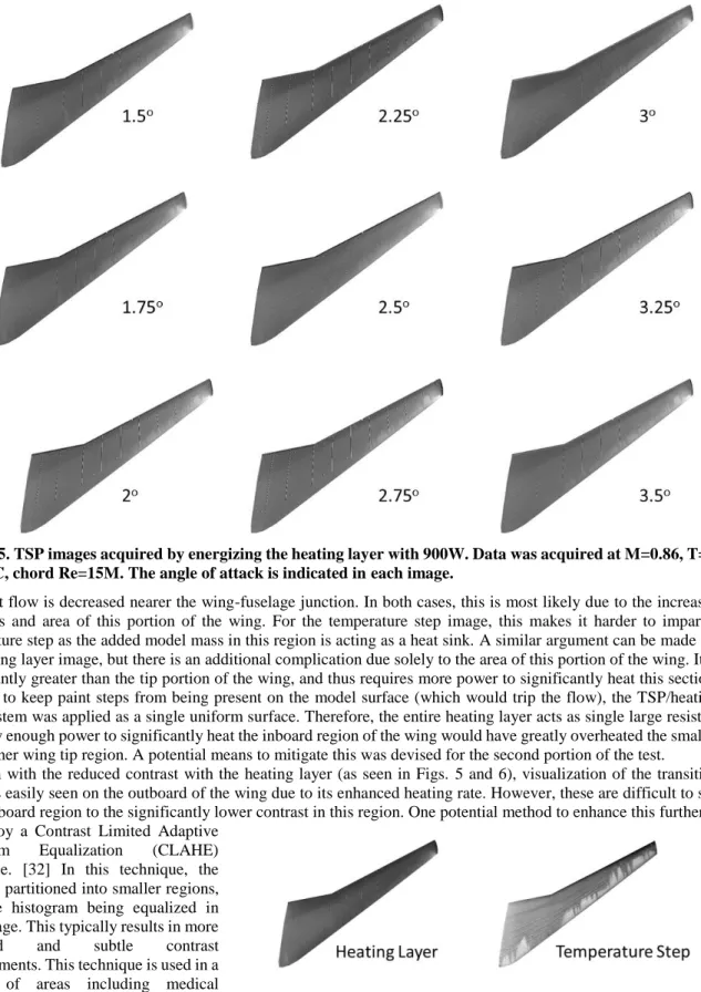
The carbon black-based heating layer was initially developed to replace a previous coating as its resistance would be higher, allowing more power to be applied using the existing power supplies. For the initial runs, data was acquired as the angle of attack was increased from 1.5o to 3.5o in 0.25o increments, for 9 total points. As described in the section above, an initial polar was acquired without the heating layer operational. After this polar, the heat was then applied (typically ~900W) and the model was allowed to heat for approximately 2 minutes. This was needed due to the larger area to be heated. After the preheat time, the model was pitched through the same angle of attack sweep. After processing the images using the steps outlined in the previous section, it was readily apparent where regions of laminar and turbulent flow existed on the wing surface. An example of the data results is shown in Fig. 5. For the figures presented in this work, the palette was adjusted so that the laminar flow regions are depicted as lighter in color than the turbulent regions.
Several observations can be made from Fig. 5. First, even with the added preheat time, the temperature change from laminar to turbulent flow is very small. In the case of the results shown in Fig. 5, the temperature change from laminar to turbulent flow is on the order of 1 oC. This is a direct result of the amount of heat that can be applied to the model. For comparison, a standard temperature step was induced into the tunnel flow by increasing the nitrogen flow, and this comparison is shown in Fig. 6. As can be seen, the contrast between laminar and turbulent flow is much greater in the case where the more traditional temperature step is employed. However, this is due to the fact that the temperature difference between laminar and turbulent flow is on the order of 2-5 oC. Careful inspection of the two images also shows other differences. First, there seems to be more turbulent wedges present in the heating layer image. This is due entirely to a flow phenomenon in the NTF. The temperature step image was acquired before the heating layer image. Several additional runs were made before the heating layer run, and at some point, damage occurred to the leading edge due to the failure of a piece of insulation in the tunnel. Second, the contrast between laminar and
turbulent flow is decreased nearer the wing-fuselage junction. In both cases, this is most likely due to the increased thickness and area of this portion of the wing. For the temperature step image, this makes it harder to impart a temperature step as the added model mass in this region is acting as a heat sink. A similar argument can be made for the heating layer image, but there is an additional complication due solely to the area of this portion of the wing. It is significantly greater than the tip portion of the wing, and thus requires more power to significantly heat this section. In order to keep paint steps from being present on the model surface (which would trip the flow), the TSP/heating layer system was applied as a single uniform surface. Therefore, the entire heating layer acts as single large resistor. To apply enough power to significantly heat the inboard region of the wing would have greatly overheated the smaller and thinner wing tip region. A potential means to mitigate this was devised for the second portion of the test.
Even with the reduced contrast with the heating layer (as seen in Figs. 5 and 6), visualization of the transition region is easily seen on the outboard of the wing due to its enhanced heating rate. However, these are difficult to see in the inboard region to the significantly lower contrast in this region. One potential method to enhance this further is to employ a Contrast Limited Adaptive
histogram Equalization (CLAHE) technique. [32] In this technique, the image is partitioned into smaller regions, with the histogram being equalized in each image. This typically results in more localized and subtle contrast enhancements. This technique is used in a variety of areas including medical imaging and microscopy. It has also been implemented in IR imaging of transition
Fig. 5. TSP images acquired by energizing the heating layer with 900W. Data was acquired at M=0.86, T=-45 oC, chord Re=15M. The angle of attack is indicated in each image.
Fig. 6. Comparison of heating layer with traditional temperature step. Conditions are the same as Fig. 5. Angle of attack is 1.5o.
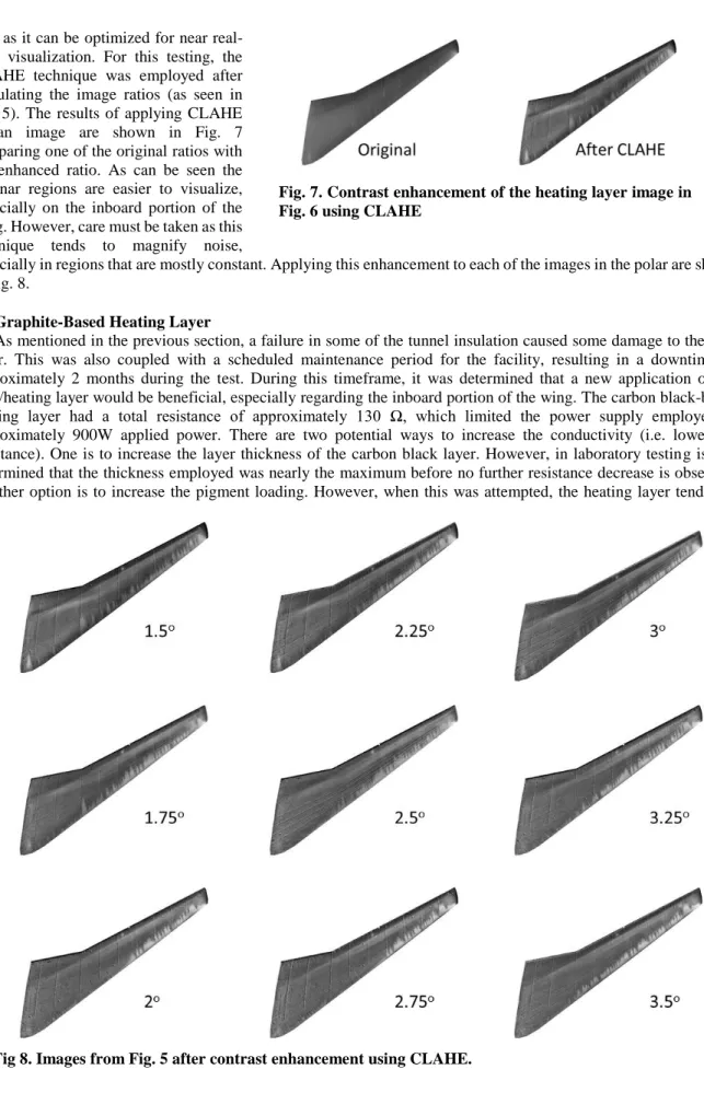
[33] as it can be optimized for near real-time visualization. For this testing, the CLAHE technique was employed after calculating the image ratios (as seen in Fig. 5). The results of applying CLAHE to an image are shown in Fig. 7 comparing one of the original ratios with the enhanced ratio. As can be seen the laminar regions are easier to visualize, especially on the inboard portion of the wing. However, care must be taken as this technique tends to magnify noise,
especially in regions that are mostly constant. Applying this enhancement to each of the images in the polar are shown in Fig. 8.
B. Graphite-Based Heating Layer
As mentioned in the previous section, a failure in some of the tunnel insulation caused some damage to the TSP layer. This was also coupled with a scheduled maintenance period for the facility, resulting in a downtime of approximately 2 months during the test. During this timeframe, it was determined that a new application of the TSP/heating layer would be beneficial, especially regarding the inboard portion of the wing. The carbon black-based heating layer had a total resistance of approximately 130 Ω, which limited the power supply employed to approximately 900W applied power. There are two potential ways to increase the conductivity (i.e. lower the resistance). One is to increase the layer thickness of the carbon black layer. However, in laboratory testing is was determined that the thickness employed was nearly the maximum before no further resistance decrease is observed. Another option is to increase the pigment loading. However, when this was attempted, the heating layer tended to
Fig. 7. Contrast enhancement of the heating layer image in Fig. 6 using CLAHE
crack when applied. Therefore, substituting carbon black with graphite was attempted. In this case, it was found that the resistance could be substantially lowered. In addition, using graphite as the pigment tended to produce an overall smoother heating layer coating than the carbon black.
While having a lower overall resistance would allow for more power to be applied, it was also desirous to be able to apply more power to the inboard region than the outboard region for reasons described in the previous section. However, since the layer had to be applied as a continuous layer, a new application protocol was devised. In this protocol, two separate graphite solutions (with different graphite loadings) were employed, as well as a gradient spraying technique. In general, more coats of the higher pigment loaded solutions were applied to the inboard portion of the model. In addition, slightly more of the heating layer was applied to the inboard section. For this test, the total thickness of
the TSP/heating layer system was approximately 400 µm on the inboard section and tapered to approximately 250 µm at the tip portion of the wing. The overall resistance of the system dropped to approximately 70 Ω. Using an alternative power supply (capable of providing up to 300V and 5.2A) would have allowed almost 1300W to be applied. However, it was decided to connect two of the existing power supplies in parallel, allowing up to 1900W to be applied.
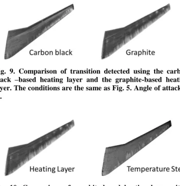
A comparison of the results from the carbon-based heating layer and the graphite-based heating layer are shown in Fig. 9. The images have been enhanced using the CLAHE technique described above. As can be seen, using the graphite-based heating layer, it is much easier to visualize the transition on the inboard portion of the wing. Considering this was a new application, a temperature step image was also acquired at these conditions to see how it compares with the heating layer. This comparison is shown in Fig. 10. While it is difficult to make specific comparisons due to the large number of turbulent wedges (which was an ongoing issue in this test and was not due to physical damage on the leading edge unlike the first portion of the test), the overall results between the two methods seem to qualitatively agree. Furthermore, in this case at least, it seems that the heating layer results are more pronounced than the temperature step results. This will be addressed in the next section.
The graphite-based heating layer was run through a variety of temperatures and Reynolds number conditions. For the lowest Reynolds number conditions (core Reynolds number of 15M at 4 oC), the transition experiments provided excellent images, as can be seen in Fig. 11. In this case, the laminar flow front is very easy to determine using the heating layer approach, especially since there are far fewer turbulent wedges at this condition. Additionally, it seems that the temperature step method actually
produces images with less contrast than the CLAHE-filtered heating layer images. To verify this, results from one of the higher Reynolds number cases (core Reynolds number of 20M at -100 oC) are shown in Fig. 12, showing that transition on the outboard of the wing is still evident, while the majority of the inboard has transitioned (except for a small
Fig. 10. Comparison of graphite-based heating layer with a traditional temperature step. The conditions are the same as Fig. 5, but with a new coating system applied.
Fig. 9. Comparison of transition detected using the carbon black –based heating layer and the graphite-based heating layer. The conditions are the same as Fig. 5. Angle of attack is 2o.
Fig. 11. Comparison of transition images collected using the heating layer and the traditional temperature step. Data was acquired at M=0.86, T=4 oC, chord Re=15M. Angle of attack
bubble right at the wing-fuselage junction). The heating layer method captured the outboard well, while this is almost absent in the temperature step method. In addition, it also shows that the graphite heating layer operates down to at least -100 oC, though this is no surprise as layers such as these have already been demonstrated down to -156 oC for transition experiments. [20,21]
C. Effect on Tunnel Measurements
One of the main concerns with using the heating layer method is the relatively
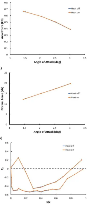
high level of power that must be applied. In initial demonstrations of the layers [19-21], this was not a critical issue as they tested areas were fairly small in area, thus mitigating the total power needed to achieve suitable heating rates. However, this work was on a much bigger scale, requiring upwards of 1900W to power properly (and could conceivably required even higher amounts). To achieve this, almost 400V was applied through the model, and there was concern about this large of voltage passing close to sensitive model instrumentation, such as the balance and the pressure transducers. To verify that voltages applied did not cause any adverse sensor readings, a comparison of data from a heat off polar and from a heat on polar were compared, and are shown in Fig. 13. As can be seen in Fig 13 (a) and Fig. 13 (b), there is no noticeable effect on the balance (which was used to calculate the axial and normal force), as there is essentially no difference in the two force measurements. In fact, the largest difference is most likely due to small changes in angle of attack between the two different polars. Likewise, the pressure transducers are measuring essentially the same pressures regardless of the heating layer status (Fig. 13 (c)).
D. Effects on Tunnel Conditions and Operation
Using the heating layer to generate the temperature step on the model should not cause any change to the actual flow conditions. To verify this, the Reynolds number measurements for each image acquired in Fig. 12 are shown in Fig. 14. For this comparison, the same number of images were acquired for the heating layer acquisition as for the temperature step acquisition (30 s total acquisition time). As can be seen in Fig. 14, the Reynolds number for the heating layer run is essentially constant, while the temperature step run has variations of up to 5%. Furthermore, the contrast of the heating layer run is actually better than that of the temperature step. Most likely a better temperature step image could have been acquired at this condition with a faster rate of change of temperature, but this would have caused an even bigger change in the Reynolds number during the run.
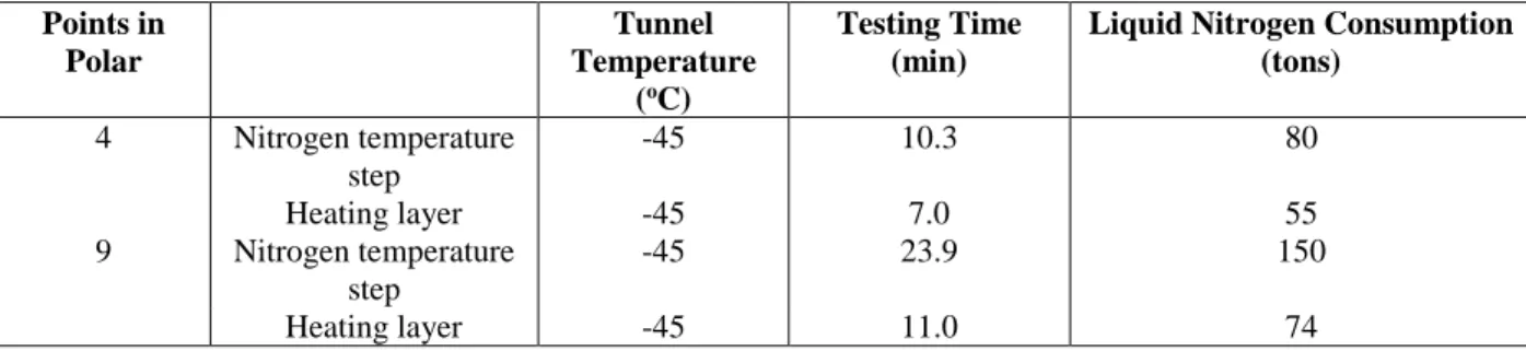
Another advantage of using the heating layer for the temperature step is an increase in tunnel operating efficiency. This should include both run time as well as liquid nitrogen usage. The savings in liquid nitrogen should be obvious; there is no increase in nitrogen usage without the nitrogen induced temperature step. For the time savings, even though there needs to be two polars run for the heating layer, there does not need to be a settling time for each point for the tunnel to recover, as is needed for the traditional temperature step run. A comparison of the two different types of polars (one with 9 points and one with only 4) is shown in Table 2.
Table 2. Testing time and liquid nitrogen consumption for the heating layer technique and traditional temperature steps Points in Polar Tunnel Temperature (oC) Testing Time (min)
Liquid Nitrogen Consumption (tons) 4 Nitrogen temperature step -45 10.3 80 Heating layer -45 7.0 55 9 Nitrogen temperature step -45 23.9 150 Heating layer -45 11.0 74
As can be seen, with a short polar (4 points), using the heating layer can improve the tunnel efficiency almost 50%. However, with longer polars (9 points), the efficiency can be increased by up to 100%.
Fig. 12. Comparison of transition images collected using the heating layer and the traditional temperature step. Data was acquired at M=0.86, T=-100 oC, chord Re=20M. Angle of attack
IV.Conclusions
This paper details the successful demonstration of a carbon-based heating layer applied to a wind tunnel model. This heating layer is used in conjunction with TSP for detection of flow transition. The more traditional w to perform this type of measurement in cryogenic facility has been to introduce a temperature step into the flow using liquid nitrogen. This has the unwanted effects of changing the flow conditions of the tunnel as well as greatly reducing testing efficiency.
The heating layer formulation is based on a polyurethane binder similar to the standard TSP formulations. However, instead of a luminescent dye dispersed in the binder, the pigment is a conductive material. For this testing, formulations using either carbon black or graphite were developed. Both pigments make a coating that has a suitable resistance (from about 50 Ω to > 200 Ω depending on pigment loading, layer thickness, etc.). The coatings are very robust to the heat that can be generated and operate in the full cryogenic conditions experienced in the NTF.
Demonstration of the coatings was performed on the CRM-NLF semi-span wing mounted in the NTF. The testing conditions for this work covered ambient temperatures down to -100 oC, requiring the development of a special TSP coating more capable of operating with this extended temperature range. The TSP/heating layer system was applied to the wing, and polished to produce a surface that was deemed suitable for transition work (Ra ~ 0.025 µm). The TSP layer was thick enough that additional polishing could be performed due to changes caused during the running of the facility.
The first coating tested was the carbon black heating layer. This performed adequately, especially when interrogating the outboard portion of the wing. However, with the increased thickness and area of the inboard region, heating this area proved difficult. To enhance the contrast, a CLAHE method was introduced as a post-processing step which greatly improved the contrast. However, it was determined that the heating layer could be improved for the second phase of the test.
Towards this goal, several improvements were made to the heating layer. First, the pigment was changed from carbon black to graphite. This served
two purposes; it decreased the resistance (to potentially allow more power to be applied with existing equipment) and it provided a generally smoother coating than the carbon black layer (which reduced preparation time). In addition, an application process was developed that significantly reduced the resistance in the inboard region compared to the outboard region. This allowed for a more constant heating over the entire surface. This coating was tested down to -100 oC, and provided excellent contrast images showing transition location. In addition, it was shown that applying the large voltage to the surface did not cause any anomalous readings from the balance or pressure transducers. Finally, looking at tunnel efficiency, using the heating layer can provide some significant operational savings, with shorter
a)
b)
c)
Fig 13. Comparison of model instrumentation readings with and without the heating layer energized. a) Axial force as measured with a lance; b) normal force as measured with a balance; c) one row of pressure transducer readings.
polars seeing up to 50% increase in efficiency, while longer polars saw 100% increase in efficiency in terms of both testing time and liquid nitrogen consumption.
Further improvements to the heating layer are possible and will be studied in the future. These include investigating other pigments (such as graphene or possibly carbon nanotubes) and developing a TSP/heating layer system that has decreased thickness (which is due to the large number of layers required to insulate the model as well as provide suitable light return to the camera). Additional tests of this heating layer concept are in development, including for rotor testing as well as a flight demonstration.
Acknowledgments
The authors would like to thank Michelle Lynde, Dick Campbell, Sally Viken, Melissa
Rivers, and David Chan at NASA LaRC for guidance and the opportunity to develop and demonstrate this technique on the semi-span model. The personnel at the NTF are also acknowledged for their assistance with the wind tunnel testing, especially Bill Goad, Scott Goodliff, and James O’Shaughnessy. Funding for this work was provided by the Advanced Air Transport Technology (AATT) Project, the Transformational Tools and Technologies (TTT) Project, and the Aerosciences Evaluation and Test Capabilities (AETC) Project.
References
[1] http://www.aeronautics.nasa.gov/aavp/aetc/transonic/ntf-quick-facts.html
[2] Sewall, W.G., Stack, J.P., McGhee, R.J., and Mangalam, S.M., “A New Multipoint Thin-Film Diagnostic Technique for Fluid Dynamic Studies,” SAE Technical Paper 881453, 1988.
doi:10.4271/881453
[3] Kuppa, S., Mangalam, S.M., Harvey, W.D., and Washburn, A.E., “Transition Detection on a Delta Wing with Multi-Element Hot-Film Sensors,” 13th Applied Aerodynamics Conference, San Diego, CA, 1995; AIAA-95-1782-CP.
doi:10.2514/6.1995-1782
[4] Olson, S.D. and Thomas, F.O., “Quantitative Detection of Turbulent Reattachment Using a Surface Mounted Hot-Film Array,”
Exp Fluids, Vol. 37, 2004, pp. 75-79. doi:10.1007/s00348-004-0786-2
[5] Dagenhart, J.R., Saric, W.S., Mousseux, M.C., and Stack, J.P., “Crossflow-Vortex Instability and Transition on a 45 Deg Swept Wing,” 20th Fluid Dynamics, Plasma Dynamics, and Lasers Conference, Buffalo, NY, 1989; AIAA-89-1892.
doi:10.2514/6.1989-1892
[6] Obara, C.J., “Sublimating Chemical Technique for Boundary-Layer Flow Visualization in Flight Testing,” J. Aircraft, Vol. 25, No. 6, 1986, pp. 493-498.
doi:10.2514/3.45611
[7] Quast, A., “Detection of Transition by Infrared Image Technique,” Proceedings of the 12th International Congress on Instrumentation in Aerospace Simulation Facilities, Williamsburg, VA, 1987, pp. 125-134.
[8] Le Sant, Y., Marchand, M., Millan, P., and Fontaine, J., “An Overview of Infrared Thermography Techniques Used in Large Wind Tunnels,” Aerospace Science and Technology, Vol. 6, 2002, pp. 355-366.
doi:10.1016/S1270-9638(02)01172-0
[9] Joseph, L.A., Borgoltz, A, and Devenport, W., “Transition Detection for Low Speed Wind Tunnel Testing Using Infrared Thermography,” 30th AIAA Aerodynamic Measurement Technology and Ground Testing Conference, Atlanta, GA, 2014; AIAA
2014-2939.
doi:10.2514/6.2014-2939
[10] Johnson, C.B., Carraway, D.L., Stainback, P.C., and Fancher, M.F., “A Transition Detection Study using a Cryogenic Hot Film System in the Langley 0.3-Meter Transonic Cryogenic Tunnel,” 25th AIAA Aerospace Sciences Meeting, Reno, NV, 1987;
AIAA-87-0049. doi:10.2514/6.1987-49
[11] Gartenberg, E. and Wright, R.E., “Boundary-Layer Transition Detection with Infrared Imaging Emphasizing Cryogenic Applications,” AIAA Journal, Vol. 32, No. 9, 1994, pp. 1875-1882.
doi:10.2514/3.1218
Fig 14. Chord Reynolds number measured during data acquisition for a heating layer run and a traditional temperature step. The conditions are the same as Fig. 12.
[12] Ansell, D., and Schimanski, D., “Non-Intrusive Optical Measuring Techniques Operated in Cryogenic Test Conditions at the European Transonic Windtunnel,” 37th AIAA Aerospace Sciences Meeting, Reno, NV, 1999; AIAA 99-0946.
doi:10.2514/6.1999-946
[13] Asai, K., Kanda, H., Kunimasu, T., Liu, T., and Sullivan, J.P., “Boundary-Layer Transition Detection in a Cryogenic Wind Tunnel Using Luminescent Paint,” J. Aircraft, Vol. 34, No. 1, 1997, pp. 34-42.
doi:10.2514/2.2132
[14] Popernack, T.G., Owens, L.R., Hamner, M.P., and Morris, M.J., “Application of Temperature Sensitive Paint for Detection of Boundary Layer Transition,” 1997 International Congress on Instrumentation in Aerospace Simulation Facilities, Pacific Grove, CA, 1997, pp. 77-83.
doi:10.1109/ICIASF.1997.644666
[15] Fey, U., Engler, R.H., Egami, Y., Iijima, T., Asai, K., Jansen, U.,and Quest, J., “Transition Detection By Temperature Sensitive Paint at Cryogenic Temperatures in the European Transonic Wind Tunnel (ETW),” 20th International Congress on Instrumentation in Aerospace Simulation Facilities, Göttingen, Germany, 2003, pp. 77-88.
doi:10.1109/ICIASF.2003.1274855
[16] Liu, T. and Sullivan, J. Pressure and Temperature Sensitive Paints (Experimental Fluid Dynamics); Springer-Verlag Berlin, Germany, 2004, pp. 8-11.
[17] Liu, T., Campbell, B.T., Sullivan, J.P., Lafferty, J., and Yanta, W., “Heat Transfer Measurements on a Waverider at Mach 10 Using Fluorescent Paint,” J. Thermophys. Heat Transf. Vol. 34, 1995, pp. 605-611.
[18] Nakakita, K., Osafune, T., and Asai, K., “Global Heat Transfer Measurement in a Hypersonic Shock Tunnel Using Temperature-Sensitive Paint,” 41st AIAA Aerospace Sciences Meeting, Reno, NV, 2003; AIAA 2003-743.
doi: 10.2514/6.2003-743
[19] Klein, C., Henne, U., Sachs, W., Beifuss, U., Ondrus, V., Bruse, M., Lesjak, R., and Löhr, M., “Application of Carbon Nanotubes (CNT) and Temperature-Sensitive Paint (TSP) for the Detection of Boundary Layer Transition,” 52nd AIAA Aerospace Sciences Meeting, National Harbor, MD, 2014; AIAA 2014-1482.
doi: 10.2514/6.2014-1482
[20] Klein, C.; Henne, U., Sachs, W., Beifuss, U., Ondrus, V., Bruse, M., Lesjak, R., Löhr, M., Becher, A., and Zhai, J., “Combination of Temperature-Sensitive Paint (TSP) and Carbon Nanotubes (CNT) for Transition Detection,” 53rd AIAA Aerospace Sciences Meeting, Kissimmee, FL, 2015; AIAA 2015-1558.
doi: 10.2514/6.2015-1558
[21] Goodman, K.Z., Lipford, W.E., and Watkins, A.N., “Boundary-Layer Detection at Cryogenic Conditions Using Temperature Sensitive Paint Coupled with a Carbon Nanotube Heating Layer,” Sensors, Vol. 16, No. 12, 2016, 2062.
doi: 10.3390/s16122062
[22] Lynde, M.N., Campbell, R.L., Rivers, M.B., Viken, S.A., Chan, D.T., Watkins, A.N., and Goodliff, S.L., “Preliminary Results from an Experimental Assessment of a Natural Laminar Flow Design Method,” AIAA Science and Technology Forum and Exposition (AIAA SciTech 2019), San Diego, CA, 2019.
[23] Gloss, B.B., “Current Status and Some Future Test Directions for the US National Transonic Facility,” Royal Aeronautical Society, London, 1992, pp. 3.1-3.7.
[24] Lynde, M.N. and Campbell, R.L., “Computational Design and Analysis of a Transonic Natural Laminar Flow Wing for a Wind Tunnel Model,” 35th AIAA Applied Aerodynamics Conference, Denver, CO, 2017; AIAA-2017-3058.
doi:10.2514/6.2017-3058
[25] Rivers, M.B., Lynde, M., Campbell, R., Viken, S., Watkins, N., and Goodliff, S., “Experimental Investigation of the NASA Common Research Model with Natural Laminar Flow Wing in the NASA Langley National Transonic Facility,” AIAA Science and Technology Forum and Exposition (AIAA SciTech 2019), San Diego, CA, 2019.
[26] Yihu, S., Xiao-Su, Y., and Yi, P., “The Electrical Self-Heating Behavior of Carbon Black Loaded High Density Polyethylene Composites,” Journal of Materials Science Letters, Vol. 19, 2000, pp. 299-301.
doi:10.1002/1099-0488(20000701)38:13<1756::AID-POLB90>3.0CO;2-P
[27] El-Tantaway, F., Kamada, K., and Ohnabe, H., “In Situ Network Structure, Electrical and Thermal Properties of Conductive Epoxy Resin-Carbon Black Composites for Electrical Heater Applications,” Materials Letters, Vol. 56, 2002, pp. 112-126. doi:10.1016/S0167-577X(02)00401-9
[28] El-Tantaway, F., Kamada, K., and Ohnabe, H., “Electrical Properties and Stability of Epoxy Reinforced Carbon Black Composites,” Materials Letters, Vol. 57, 2002, pp. 242-251.
doi: 10.1016/S0167-577X(02)00774-7
[29] Crouch, J.D., Sutanto, M.I., Witkowski, D.P., Watkins, A.N., Rivers, M.B., and Campbell, R.L., “Assessment of the National Transonic Facility for Laminar Flow Testing,” 48th AIAA Aerospace Sciences Meeting, Orlando, FL, 2010; AIAA 2010-1302.
doi:10.2514/6.2010-1302
[30] Watkins, A.N., Buck, G.M., Leighty, B.D., Lipford, W.E., and Oglesby, D.M., “Using Pressure- and Temperature-Sensitive Paint on the Aft-Body of a Capsule Entry Vehicle,” AIAA Journal, Vol. 47, No. 4, 2009, pp. 821-829.
doi:10.2514/1.37258
[31] Egami, Y., Fey, U., and Quest, J., “Development of New Two-Component TSP for Cryogenic Testing,” 45th AIAA Aerospace Sciences Meeting, Reno, NV, 2007; AIAA 2007-1062.
[32] Zuiderveld, K., “Contrast Limited Adaptive Histogram Equalization,” Graphics Gems IV, edited by Paul S. Heckbert, Academic Press International, Inc., San Diego, CA, 1994, pp. 474-485.
[33] Garbeff, T.J. and Baerny, J.K., “Recent Advances in the Infrared Flow Visualization System for the NASA Ames Unitary Plan Wind Tunnels,” 55th AIAA Aerospace Sciences Meeting, Grapevine, TX, 2017; AIAA-2017-1051.