S E D A P
A PROGRAM FOR RESEARCH ON
S
OCIAL AND
E
CONOMIC
D
IMENSIONS OF AN
A
GING
P
OPULATION
International Differences in Longevity and Health
and their Economic Consequences
P.-C. Michaud
D. Goldman
D. Lakdawalla
A. Gailey
Y. Zheng
For further information about SEDAP and other papers in this series, see our web site: http://socserv.mcmaster.ca/sedap
Requests for further information may be addressed to: Secretary, SEDAP Research Program
Kenneth Taylor Hall, Room 426 McMaster University Hamilton, Ontario, Canada
L8S 4M4 FAX: 905 521 8232 e-mail: [email protected]
September 2009
The Program for Research on Social and Economic Dimensions of an Aging Population (SEDAP) is an interdisciplinary research program centred at McMaster University with co-investigators at seventeen other universities in Canada and abroad. The SEDAP Research Paper series provides a vehicle for distributing the results of studies undertaken by those associated with the program. Authors take full responsibility for all expressions of opinion. SEDAP has been supported by the Social Sciences and Humanities Research Council since 1999, under the terms of its Major Collaborative Research Initiatives Program. Additional financial or other support is provided by the Canadian Institute for Health Information, the Canadian Institute of Actuaries, Citizenship and Immigration Canada, Indian and Northern Affairs Canada, ICES: Institute for Clinical Evaluative Sciences, IZA: Forschungsinstitut zur Zukunft der Arbeit GmbH (Institute for the Study of Labour), SFI: The Danish National Institute of Social Research, Social Development Canada, Statistics Canada, and participating universities in Canada (McMaster, Calgary, Carleton, Memorial, Montréal, New Brunswick, Queen’s, Regina, Toronto, UBC, Victoria, Waterloo, Western, and York) and abroad (Copenhagen, New South Wales, University College London).
International Differences in Longevity and Health
and their Economic Consequences
P.-C. Michaud
D. Goldman
D. Lakdawalla
A. Gailey
Y. Zheng
International Differences in Longevity and Health and their Economic Consequences
P.-C. Michaud, D. Goldman, D. Lakdawalla, A. Gailey, Y. Zheng RAND Corporation1
June 2009
Abstract
In 1975, 50 year-old Americans could expect to live slightly longer than their European counterparts. By 2005, American life expectancy at that age has diverged substantially compared to Europe. We find that this growing longevity gap is primarily the symptom of real declines in the health of near-elderly Americans, relative to their European peers. In particular, we use a microsimulation approach to project what US longevity would look like, if US health trends approximated those in Europe. We find that differences in health can explain most of the growing gap in remaining life expectancy. In addition, we quantify the public finance consequences of this deterioration in health. The model predicts that gradually moving American cohorts to the health status enjoyed by Europeans could save up to $1.1 trillion in discounted total health expenditures from 2004 to 2050.
Keywords: disability, mortality, international comparisons, microsimulation
JEL Codes: I10, I38, J26
1 We thank the Department of Labor and the National Institute of Aging for financial support. We also thank Michael Hurd, James Smith, Maggie Weden and Arthur van Soest as well as seminar participants at Tilburg University and the Michigan RRC. Corresponding author: Pierre-Carl Michaud, 1776 Main Street, Santa Monica, CA 90401: [email protected].
Résumé
En 1975, l’espérance de vie d’un américain âgé de 50 ans était pratiquement la même que celle d’un européen. En 2005, on pouvait constater que l’espérance de vie aux États-Unis avait considérablement divergé de celle observée en Europe. Nous rapportons que ce retard est en grande partie le résultat d’un déclin important de la santé de la population américaine approchant l’âge de la retraite. Nous utilisons un modèle de microsimulation pour prédire l’espérance de vie aux États-Unis sous l’hypothèse que les américains approchant la retraite partagent le même état de santé que la population européenne. Un de nos résultats important est que la différence d’espérance de vie entre américains et européens peut être entièrement expliquée par ces différences de santé aux alentours de l’âge de 50 ans. De plus, nous quantifions les conséquences économique des cette détérioration de la santé aux États-Unis. Notre modèle prédit que de graduellement faire converger la population américaine vers un niveau de santé équivalent à celui des européens pourrait avoir pour conséquence de réduire les dépenses de santé de $1.1 trillion entre 2004 et 2050.
A.
Introduction
The populations of the United States and Western Europe have experienced large gains in life-expectancy over the last century. For example, U.S. life expectancy at birth increased from 61 years in 1933 to 78 years in 2004.2 In most developed countries, age-specific death rates have declined exponentially at a constant rate (Tuljapurkar et al., 2000). Large declines in infectious diseases drove down mortality rates during the first half of the 20th century, particularly for the young. During this period, life expectancy across developed countries also converged (White, 2002).
The second half of the 20th century witnessed continued growth in longevity, but of a much different nature. Reductions in mortality among the elderly, rather than the young, dominated movements in life expectancy (Olshansky and Carnes, 2001). During this era, another difference emerged: the US began to fall behind other developed countries in terms of life expectancy (Oeppen and Vaupel, 2002). So far, little is known about the causes of this widening gap (Lee, 2003).
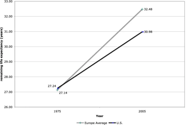
According to the Human Mortality Database (HMD), in 1975, life expectancy at age 50 was similar in the US and Europe. Americans lived on average 27.3 years, compared to 27.1 years for a representative group of Western European countries (Denmark, France, Italy, The Netherlands, Spain and Sweden).3 Over the ensuing
decades, however, European life expectancy grew more quickly. As Figure 1 shows, a 50 year-old American in 2004 could expect to live 31 years, compared to 32.5 years in Europe. A difference of 1.5 years in life expectancy implies a non-trivial welfare loss. For example, using $100,000 as a lower-bound estimate of the value of a statistical life year (Viscusi and Aldy, 2003), this represents at least a $700 million dollar disadvantage for the current generation of 50 year olds. While the cross-country longevity gap remains smaller than within-country differences along the lines of socioeconomic status, the
2 Based on life tables collected in the Human Mortality Database (www.mortality.org).
3 We used period life-table data from the Human Mortality Database (HMD, www.mortality.org). The HMD did not have data going back to 1975 for Germany.
surprise lies in the divergent paths of the US and Europe, in spite of their similar levels of economic development.
Over that same period, chronic illnesses associated with more sedentary lifestyles have spread, somewhat mitigating improvements in life expectancy (Goldman et al., 2005; Lakdawalla et al., 2005). Due to data limitations, it is hard to assess whether trends in chronic disease have spread more rapidly in the US, but historical data do exist on risky health behaviors that contribute to chronic disease. Using data from the OECD, Figure 2 shows tobacco consumption per capita (1960-2005) and obesity rates for the U.S. and European countries where data exist (1978-2005). While tobacco consumption is higher in Europe today, it was much higher in the US for the earliest years in the figure. While near-elderly Americans are less likely to be smoking now than their European counterparts, they are much more likely to have ever smoked. One plausible explanation for this rapid decrease is that smoking cessation programs have been more effective in the U.S. than in Europe but that take up as started earlier. For example, Cutler and Glaeser (2006) argue that 50% of the gap in current smoking status is due to
differences in beliefs about the health effects of smoking, Europeans thinking it is not as harmful for health as Americans do.
The second panel shows the obesity rate, defined as BMI>30, for the U.S. and a set of European countries for whom data is available. Both the level and slope are larger in the U.S. The U.S. and Europe have diverged starkly since the 70s.4 Reduction in the costs of food consumption and technological innovation which led to more sedentary work are two key explanations put forward to explain the U.S. trend (Lakdawalla and Philipson, 2002). Cutler et al. (2003) argue that these changes may have taken place more slowly in Europe due in particular to stricter food regulation.
Figure 3 displays what are perhaps the consequences of these divergent trends; the US prevalence of chronic disease and risky behavior is much higher than in European countries (Banks et al., 2006; Andreyeva et al., 2007). The figure displays these data
4 Data based on measured weight and height rather than self-reported. Data for the U.S. is from the NHANES survey. The OECD and WHO harmonize these measures across countries for survey and
among the 50-55 year old population using internationally comparable survey data.5 Except for current smoking status, Americans look worse in terms of health. Several of the differences are quite large. For instance, Americans are about twice as likely to have hypertension, twice as likely to be obese, twice as likely to have diabetes, and nearly 50% more likely to have ever smoked, As we demonstrate latter, these differences are
unlikely to be explained by differences in diagnosis or reporting. For example, the prevalence of stroke is twice as low in Europe as in the U.S., a condition which rarely goes undiagnosed.
Clearly, the apparent gaps in observed health status would contribute to a gap in longevity, but it is not obvious how big the contribution will be. For instance, there are well-documented longevity gaps across racial and socioeconomic lines, within countries. These are not fully explained by differences in observed health status. The question is whether “being American” is an independent mortality risk factor, in the same way that being poor or being black increase risk above and beyond observed health.
Furthermore, it is worth considering the fiscal consequences of these trends as the United States and Europe begin to grapple with the consequences of shifting population demographics. On the one hand, decreased longevity—especially due to higher mortality at older ages—can ease the burden on public pension programs such as Social Security and public insurance. However, if the longevity decrease comes at the expense of increased chronic disease and disability, then there is increased pressure on public health insurance and disability insurance programs. The net effects then are unclear.
This paper aims to address this and several related questions. First, we assess whether differences in near-elderly health are enough to explain the longevity gap across countries. From a policy perspective, it is important to know whether differences in life expectancy are due to differences in health before or after age 50. The answer to this question identifies the target population for health interventions, and provides insight into the relative value of preventive or curative care. While consistent historical data on health
5 We used the 2004 waves of the Health and Retirement Study in the U.S. and the Survey of Health Ageing and Retirement in Europe to produce these numbers. Properly weighted, both surveys are representative of the age 50+ population in each country. Questions on health conditions are very similar. The text of those questions is reproduced in Table A.1 of the appendix.
conditions are unavailable across countries, we use a dynamic microsimulation model calibrated to match historical U.S. health and longevity dynamics over the life course. We then simulate a counterfactual where the health of an American cohort mimics the health of Europeans observed in 2004. Second, we quantify the fiscal consequences of
differences in health and longevity across countries, using the detailed policy modules from the micro simulation model.
The paper is structured as follow. Section B describes the model that is used to describe the long-term economic consequences of these trends. Section C uses the model to quantify the effect of differences in health on longevity and government
expenditures/revenues, and Section D discusses the results.
B.
Microsimulation Model of Health and Economic Dynamics
B.1 Background
To link morbidity to longevity, one needs a transition model that relates current health to the future risk of mortality. Given our interest in fiscal consequences, we also need a model linking health and economic outcomes. Both the epidemiological and economic literatures contain complex models of each, but few integrate both.
The current social science literature features several well-known and
complementary approaches for measuring population health and projecting future disease burden and mortality—including models by Manton and co-authors (Manton, Singer et al. 1993), Lee (Lee 2000), and Hayward (Hayward and Warner 2005). Across these models, there is an underlying trade-off between the complexity of the data required, and the broad applicability of the model. For instance, early life table approaches like those of Sullivan (1971) require only age-specific population data as well as corresponding disability rates at those same ages; these elements are all present in cross-sectional data. However, these straightforward data requirements come at a cost, as the Sullivan method appears too insensitive to large changes in disability and mortality, and may thus
underestimate future trends in population health (Bonneux, Barendregt et al. 1994). Multistate life table models and microsimulation models that exploit longitudinal data, however, can accommodate richer dynamics than Sullivan’s method and thus provide
more flexibility in modeling the dynamic interplay between morbidity, disability, and mortality. Such dynamic models obtain population health trends as aggregates from individual stochastic processes underlying these outcomes.
We use a model that considers the dynamic interplay between a large number of health outcomes as well as economic outcomes. The model is an extension of the Future Elderly Model (FEM) (Goldman, Hurd et al. 2004). This is a reduced-form markovian model that allows for unobserved heterogeneity and correlation across outcomes. In that sense, it is well equipped to analyze the effect of the health differences on longevity and public financial liabilities, as it allows for complex interactions between
multi-dimensional measures of health and economic outcomes.
B.2 Functioning of the Dynamic Model
B.2.1 Overview
The Future Elderly Model (FEM) was developed to examine health and health care costs among the elderly Medicare population (age 65+) (Goldman, Hurd et al. 2004). The FEM has been used to assess the technological risk facing Medicare(Goldman, Shang et al. 2005), to forecast the costs of obesity in older Americans (Lakdawalla, Goldman et al. 2005); to model disability-related trends (Chernew, Goldman et al. 2005); to examine the future costs of cancer (Bhattacharya, Shang et al. 2005); to estimate the value of
preventing disease after age 65 (Goldman, Cutler et al. 2006), and to compare the impact of pharmaceuticals on longevity in Europe and the United States (Lakdawalla, Goldman et al. 2009). The most recent version now project these outcomes for all Americans aged 50 and older using data from the Health and Retirement Study. The defining
characteristic of the model is the use of real rather than synthetic cohorts, all of whom are followed at the individual level. This allows for more heterogeneity in behavior than would be allowed by a cell-based approach. The model has three core components:
The initial cohort module predicts the health and socio-economic outcomes of new cohorts of 50 year-olds. This module calibrates the Health and Retirement Study (HRS) to reflect population trends observed in younger populations from the National Health Interview Study (NHIS). It allows us to generate new cohorts as the simulation proceeds, so that we can measure outcomes for the age 50+ population in any given year.
The transition module calculates the probabilities of entering and exiting various health states, and the likelihood of various financial outcomes. The module takes as inputs risk factors such as smoking, weight, age and education, along with lagged health and financial states. This allows for a great deal of heterogeneity and fairly general feedback effects. The transition probabilities are estimated from the longitudinal data in the Health and Retirement Study (HRS). These probabilities are then used to simulate the path of individuals in the simulation.
The policy outcomes module aggregates projections about individual-level outcomes into policy outcomes such as taxes, medical care costs, pension benefits paid, and disability benefits. This component takes account of public and private program rules to the extent allowed by the available outcomes. Because we have access to HRS-linked restricted data from Social Security records and employer pension plans, we are able to realistically model retirement benefit receipt.
Figure 4 provides a schematic overview of the model. We start in 2004 with an initial population aged 50+ taken from the HRS. We then predict outcomes using our estimated transition probabilities. Those who survive make it to the end of that year, at which point we calculate policy outcomes for the year. We then move to the following year, when a new cohort of 50 year-olds enters (with a different health profile). These entrants, along with the survivors from the last period, constitute the new age 50+ population, which then proceeds through the transition model as before. This process is repeated until we reach the final year of the simulation. The model can be run for a single cohort, without entering cohorts, or at the population level where successive cohorts enter the simulation. In the population-level simulation, we can track both population as well as cohort outcomes. In what follows we give an overview of each component of the model. The technical appendix accompanying this paper contains more details on the implementation.
B.2.2 Initial Cohort Module
We aim to characterize outcomes for the age 50+ population. Hence, we need to predict the characteristics of the current and future 50 year-old population, in terms of health, demographics and economic outcomes. Unfortunately, the HRS does not include respondents younger than age 50; therefore, the characteristics of future 50 year-olds
must be modeled using data on younger individuals. It is not sufficient to merely replicate the 50-year olds observed today because of the non-stationarity of health in younger populations.
We estimate trends in the health of 50 year-olds using two methods. First, we use the method described in Goldman, Hurd et al. (2004) to calculate trends in disease prevalence from the National Health Interview Surveys (NHIS). The trends we estimate are relatively close to other independent estimates, as documented in the appendix. For outcomes other than disease prevalence, we use existing estimates, all of which are documented in the technical appendix.
Second, we use the 50 year-old HRS respondents from 2004 as a template for future cohorts of 50 year-olds. We adjust their health to match projected prevalence levels, using the trends estimated in the first step. For example, if obesity is projected to rise in 2020, we increase the rate of obesity within the cohort of 50 year-olds, by
reassigning enough non-obese individuals to obesity status. Since obesity is correlated with other outcomes such as hypertension and diabetes, we reassign obesity status so that those at greatest risk are more likely to acquire it.
The reassignment is governed by a latent health model with correlated unobservables. An individual’s disease status is a function of the mean population probability of the disease, along with a random error term. For an individual, the error terms are correlated across diseases. This builds in the possibility that, for instance, the occurrence of diabetes and hypertension are correlated. We jointly estimate the
population means and the covariance structure of the error terms by maximum simulated likelihood (more details appear in the technical appendix). Table 1 lists all the outcomes that we model. There are seven binary outcomes: hypertension, heart disease, diabetes, fair or poor self-reported health, labor force participation, insurance status and positive wealth. (The inclusion of this last indicator is necessary because of the observed spike in the distribution of net wealth at zero in the HRS.) There are three ordered outcomes: BMI status, smoking status and functional status in the transition model. Finally, there are five continuous outcomes: average indexed monthly earnings (AIME), the number of quarters of coverage; earnings, financial wealth, and defined contribution (DC) wealth. We also model respondents’ pension plan outcomes: whether they have a defined benefit
(DB) or DC plan on the current job; the earliest age at which they are eligible; and the conventional retirement age. We group the latter around peaks in the empirical
distribution. The most common early retirement age is 55, and the modal retirement age is 62. Finally, each of these outcomes depends on fixed characteristics such as race, education, gender and marital status. We also consider cancer, lung disease and stroke as fixed covariates, because their prevalence is very low in this population (age 50-53). Estimates are presented in the appendix.
Finally, the size of the entering cohort is adjusted to reflect population projections from Census by gender and race. We also adjust the size of the initial new cohort in 2004 to Census estimates by gender, race and ethnicity.
B.2.3 Transition Model
The transition model tracks movement among states as a function of risk and demographic factors. The technical appendix provides details on the parametric
structure, estimation, and validation of the model. Here we enumerate and discuss all the key inputs and outputs of the model, and how they are measured.
The data come from the 1992 to 2004 biennial waves of the HRS. We consider both health and economic outcomes, all of which are listed in Table 2. The table lists several groups of variables: diseases, risk factors, functional status, labor force and benefit status, financial resources, nursing home residence, and death. At a particular point in an individual’s life, the model takes as inputs the individual’s risk factors, along with her lagged disease status, functional status, labor force and benefit status, financial resources, and nursing home status. The outputs are current disease status, functional status, labor force and benefit status, financial resources, and nursing home status. More detail on variable measurement is presented below.
Transition rates are allowed to differ across demographic and economic groups. In particular, we allow differences by gender, race and ethnicity, education, and marital status. Transition equations are estimated on 7 waves of the HRS. We assess the fit of the model by simulating 2004 outcomes for the 1992 HRS respondents; these are then compared actual outcomes. We use half the sample for estimation and the other half for simulation. In general, the model fits the data quite well, with a close correspondence
between predicted and actual outcomes in most areas. Complete results can be found in Table A.9 of the technical appendix.
Measurement of Variables
The list of diseases includes the most prevalent conditions in the HRS survey: hypertension, stroke, heart disease, lung disease, diabetes and cancer. An individual’s disease status is estimated using the responses to questions of the form: "Has a doctor ever told you that you had…." Consistent with the chronic nature of these illnesses, we assume there is no chance of recovery and model the time until diagnosis (after age 50).
Second, we consider risk factors, focusing particularly on smoking and obesity. We model transitions across three “obesity” states: not obese (BMI<25), overweight (25-30) and obese (BMI>(25-30). This information is derived from self-reports on weight and height; while not as accurate as physical measurement, they are nonetheless highly predictive of population outcomes. For smoking, we model whether the respondent: has never smoked, has ever smoked but quit, or is still smoking at the time of the interview.
Third, we measure functional status using ADL (activities of daily living) and IADL (instrumental activities of daily living) limitations. These are counts of positive answers to questions (5 for ADL limitations and 7 for IADL limitations) such as whether the respondent has trouble walking, getting out of bed, dressing, etc. IADLs are typically less severe impairments than ADLs. We measure functional status by classifying
respondents into the following categories: no IADL or ADL limitations, 1-2 IADL limitations but no ADL limitations, 1-2 ADL limitations, or 3+ ADL limitations. This classification scheme yields four mutually exclusive categories (based on the data). These are not assumed to be absorbing states in that we allow for recovery.
Next, we add labor force and benefit receipt outcomes. (We express all monetary units in terms of 2004 dollars using the Consumer Price Index.) First, we track whether someone works for pay (any positive hours), and we track earnings on the main job. We also track whether the respondent has employer-based health insurance, or derives coverage from other sources (apart from Medicare). We do this for the population younger than age 65. After age 65, nearly all respondents have insurance through Medicare. An individual can derive coverage through his employer, the employer of his/her spouse, a private insurer, or a government assistance program such as Medicaid
(if disabled). We also record whether someone has a pension on his job, and whether this is a defined benefit (DB) or defined contribution (DC) type. If the respondent reports a DC pension, we also consider the self-reported account balance as another dependent variable. If the respondent reports a DB pension, we record the earliest age at which the pension can be claimed, as well as the number of years on the job and the normal
retirement age on that plan. We also construct a variable recording whether someone is claiming a DB pension on the current job (quitting a job with a DB pension). Hence, we have two binary state variables (DC and DB entitlement) and one continuous state-variable (DC account balance) to take account of private pensions.
We model Social Security retirement benefit receipt using the self-reported age at which benefits were first claimed. Since we have access to earnings records for
respondents in the HRS, we also determine who is eligible upon reaching age 62 using quarters of coverage. We construct the Average Indexed Monthly Earnings (AIME) for the initial interview and update the AIME in the simulation using a simplified rule as in French (2005).6 The AIME is the basis for computing benefits. We also model disability insurance (DI) benefit receipt and Supplemental Security Income (SSI) using self-reports from the HRS. When reporting SSI figures however, we use a measurement error
correction model estimated from merging self-reported with administrative data from SSA to correct for underreporting (see Technical Appendix for details).
We then add measures of financial resources. We construct a measure of net financial wealth using self-reports from the HRS and imputations performed by RAND (Hurd, Hoynes et al. 1998). Net financial wealth is defined as the value of financial assets (checking, savings, stocks, IRAs, Certificate deposits, bonds) plus the value of real assets (primary house, other real estate, other real assets) minus all debt (mortgage, home loans, credit cards, etc). We also track earnings, and whether wealth is positive. To account for the skewness of the wealth and earnings distribution, we use the generalized inverse hyperbolic sine transformation. For both wealth and earnings, we censor observations above the 99th percentile in 2004.
6 We estimate a regression function of next period’s AIME as a function of baseline AIME and earnings. We allow coefficients to be age specific and consider a second-order approximation. Estimates available upon request.
Finally, we track nursing home residence, and mortality. The HRS initially did not sample from the nursing home population. Because our simulations typically start at age 50, this is not a major limitation. More importantly, the HRS follows respondents into nursing homes and also records transition back to independent or assisted living outside nursing homes. Mortality is recorded in exit interviews in the HRS. Mortality hazards derived from the HRS correspond closely with life-table probabilities (Adams, Hurd et al. 2003; Michaud, Kapteyn et al. 2006)).
Model Restrictions
We make several restrictions on the transition risks permitted in the model. First, we only allow feedback from diseases where clinical research supports such a link based on consultation with several physicians from the Southern California Evidence-Based Practice Center. For example, we allow hypertensive patients to have higher risk of heart disease, but we do not allow hypertensive patients to have higher risk of cancer. These clinical restrictions are documented in the technical appendix and elsewhere (Goldman, Hurd et al. 2004).
Another important restriction we impose is that economic outcomes do not feedback to health. This is consistent with the findings from previous studies (Adams, Hurd et al. 2003). SES does not appear to have a causal effect on health outcomes in this age range. The correlation between SES and health appears to be generated by feedback effects from health to economic status, most notably through the effect of health shocks on labor supply and medical spending. Also playing a role are predetermined (earlier) events or common factors (genetics, etc) that induce a non-causal correlation between SES and health. These two factors are accounted for in the estimation.
B.2.4 Policy Outcomes
The model simulates a number of relevant health and economic outcomes for individuals. First, we consider a set of health outcomes such as life expectancy, healthy life
expectancy (no ADL limitations), and medical expenditures. Average medical expenditures by disease and demographic group are calculated from two sources. For those younger than age 65, we use the Medical Expenditure Panel Survey (MEPS) and include in medical expenditures the respondents’ medical care costs and the cost of drugs. For those above age 65, we use the Medicare Current Beneficiary Survey (MCBS). The
MEPS is known to under-predict expenditures compared to National Health Expenditure Accounts (NHEA) (Sing et al., 2006). We also find that the MCBS under-predicts expenditures from the NHEA. Without adjustment, we seem to under predict payments (by $59 billion for Medicare and $38 billion for Medicaid). Our cost estimates are based on average expenditures in the Medical Current Beneficiary Survey (MCBS) and total costs in the MCBS are also lower than in the NHEA. The MCBS is known to undercount medical spending by both the Congressional Budget Office and the CMS (Christensen and Wagner 2000).7 Hence, we adjust those numbers to match the NHEA, inflating costs by 15%. More detail can be found in the Appendix (section 5, p. 12).
In addition to the individual outcomes, the model predicts revenues and expenditures by the Federal Government, for the age 50+ population. As part of the predicted medical expenditures, we also predict expenditures by source, including those by Medicare and Medicaid. Next, we compute Social Security retirement benefits for those predicted to receive such benefits. Since we have the AIME of both respondent and spouse, we can precisely estimate the distribution of retirement benefits. We account for spouse and survivor benefits. We also compute disability insurance (DI) benefits and Supplemental Security Income (SSI). As Michaud et al. (2009) report, the simulation is able to replicate basic fiscal aggregates for 2004. We compute DB pension income from average pension payments by tenure, last earnings and early and normal retirement ages using Pension Plan characteristics reported by Employers of HRS respondents. Using all these income flows, for the respondent and the spouse (if present), we compute net household income where taxes include Federal, State, City income taxes as well as the Social Security taxes (OASDI and Medicare). More detail is provided in the appendix. B.2.5 Simulation Methods
For population scenarios, the simulation starts with the existing age 50+ population in the 2004 wave of the HRS. The microsimulation is stochastic, meaning that transitions are randomly drawn from the joint distribution of state variables which is estimated from the HRS. There are two stochastic elements in the model: the simulation of new cohorts and the simulation of transitions. To generate new cohorts, we make use of the estimated joint
7The Congressional Budget Office, for example, inflated MCBS prescription drug spending by 15 percent to produce its official forecast of the cost of Part D.
distribution and use random draws from the correlated errors to generate a new cohort. Second, for each respondent in a given year, we calculate transition probabilities. We then draw random numbers to attribute new outcomes. This process is repeated a number of times to ensure independence from any particular sequence of random numbers. We average over 10 replications. For cohort scenarios, we only use the 2004 age 50 cohort and simulate outcomes until everyone has died.
C.
Results
As noted earlier, our objectives are to assess whether health differences explain the longevity gap, and to quantify the fiscal consequences of gradually closing the health gap. To meet the first objective, we examine the 2004 cohort of 50 year-olds, and consider the counterfactual in which Americans have the same health as Europeans. The resulting longevity is compared to the longevity predicted using the baseline health status of Americans. We also assess the total differences in public spending generated by these underlying differences in health. The second experiment requires analyzing population-level projections for health and economic outcomes if we gradually moved American health levels to those of Europeans.
C.1 Explaining Longevity Differences
We use the prevalence rates presented in Figure 3 to construct the first counterfactual cohort. We simulate the baseline outcomes of the cohort using the adjusted prevalence rates from European data. Using the methodology outlined in B.2.2, we preserve the correlation between health and other outcomes in the model. We keep other socio-economic characteristics constant at American levels while varying health status of the cohort. We then simulate transitions until every one dies in the simulation. We compare this counterfactual with the status quo case where American health is unchanged.
Our baseline projection of remaining life-expectancy at age 50 is 31 years. This is very close to the 30.98 years estimate from life tables presented in Figure 1. In Figure 5, assigning European health status levels to Americans increases healthy life expectancy (years without ADLs) by 1.3 years, and decreases unhealthy life expectancy (years with 1+ ADLs) by a tenth of a year. The overall effect is to increase life expectancy by 1.2
years, which is 92% of the difference in life expectancy reported in World Health Organization data.
These gaps in health and longevity have important fiscal consequences. The resulting change in life expectancy may increase both revenues and expenditures, while possibly reducing medical care costs. Table 3 computes the overall fiscal effects on a per capita basis. Revenue would increase by $2,425 per capita, partly due to the increase in life expectancy and increase in earnings/labor force participation. On the expenditure side, there are two effects. First, old age pension benefits increase by a substantial
amount ($6593 per capita). This is roughly the size of the average annual Social Security benefit payment. But, there is a larger decrease in Medicare, Medicaid and Disability insurance (DI) benefit payments. Total lifetime health care expenditures decrease by a stunning $17,791. This represents an 8.5% reduction in lifetime medical expenditures. The average reduction in lifetime payments is $4,717 for Medicare and $3,687 for Medicaid. Adding the reduction in DI costs, the net effect on government expenditures is $2,477 per capita. Overall the net fiscal impact of this scenario is an increase in per capita net revenue of $4,902 for the government.
C.2 Long-Term Financial Consequences
The experiment above computes the contribution of health differences to longevity, and public spending. We are also interested in the more practical question concerning the consequences of gradually, rather than immediately, moving cohorts of near-elderly Americans towards the health status of their European counterparts.
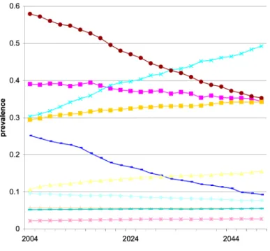
To implement a gradual scenario we allow prevalence rates in the entering cohort to reach European levels by 2030. This is compared to a status quo scenario in which current trends observed and projected among the new elderly persist. Hence, this scenario can be interpreted as a transition from the current steady-state to a new one. The fiscal effects have a direct economic interpretation for policies that would help reach that steady-state. Figure 6 provides the time path for various conditions among entering cohorts in the baseline and the counterfactual scenario. Each year, the population alive is representative of the age 50+ population alive in the U.S.
We report the results for the status quo in Table 4. Given current trends, we project the size of the population aged 50+ will increase by nearly 75% from 80.7 million in 2004 to 144 million in 2050. The population forecast for 2050 is very close to that of the Social Security Administration (80.8 million). Life expectancy is projected to
increase from 31 years in 2004, to 31.6 years in 2050. However, as estimated in Michaud et al. (2009), this improvement is likely to coincide with more time spent in a disabled state, since disability-free life expectancy is projected to be lower in 2050.
We compare the baseline to the scenario described in Figure 6, of gradual movement towards European prevalence levels. Table 5 reports the results. Because of longevity gains, the population age 50+ is 4%, or 5.75 million, larger in 2050. The population is also much healthier in 2030 and 2050 than under the status quo. For example, the obesity rate falls by 24 percentage points, while the prevalence of lifetime smoking and of diabetes both fall by roughly 10 percentage points each.
Government revenue rises by 10%, or $30 billion, by 2050, as a result of the longevity gains. As before, there are two offsetting expenditure effects. On one hand, longer lives imply larger annuity burdens: OASI benefits go up by $70.4 billion. On the other hand, medical costs decrease by $124 billion, or 6.7%, in 2050. Medicare saves $36.4 billion despite the increase in longevity. The overall effect on expenditures is initially negative, but turns positive by 2050. As found in Michaud et al. (2009), a transition to better health first decreases expenditures, but gains in longevity eventually exert upward pressure on spending.
In Figure 7, the gains in health expenditure materialize quickly, while the annuity burden takes longer to emerge. This is essentially a timing issue, cost savings due to lower disability appear before extensions in life expectancy. The total effect on expenditures is largest around 2030 and goes to zero by 2050. Since revenue rises as well, the net fiscal effect is positive in 2050 but slowly converging to zero. Hence, the transition to better health involves important fiscal effects, but these largely vanish once the new equilibrium is reached.
Figure 8 shows that, in present value terms from the 2004 perspective, the increase in tax revenue almost entirely offsets the annuity burden. The effect on health expenditures remains. The present discounted value of Medicare and Medicaid savings
combined is $632 billion, or 1.6 years of combined 2004 spending on the two programs. In terms of total medical spending, the present value of those savings is $1.1 trillion dollars.
C.3 Robustness to Cross-Country Differences in Diagnosis
An alternative interpretation of cross-country differences in health focuses on differences in rates of diagnosis, rather than real differences in health status. The literature
documents under-diagnosis of diseases like diabetes and hypertension in the US (Smith, 2007), but it is difficult to find comparable European studies. However, one direct analysis of this question suggests that differences in diagnosis are relatively modest. Banks et al. (2006) compare objective clinical diagnosis among men, using commonly used thresholds on biomarkers, to self-reports of whether respondents have previously been diagnosed. For diabetes among those aged 40-70, they find a clinical prevalence of 4.8% in the UK and 8.9% in the US, but self-reported prevalence of 4.4% and 8.6%, respectively. The cross-country difference is similar using self-reports or clinical measurements (4.2% versus 4.1%). They find a similar result for hypertension. These discrepancies are not large relative to the differences we observe in the data.
Of course, the Banks et al. evidence is somewhat narrow in its focus on diabetes and hypertension, and on the US-UK difference specifically. To test the sensitivity of our results to diagnostic differences, we ran the cohort analysis under various assumptions about differential diagnosis. We defined 6 scenarios in which the difference between the U.S. and Europe prevalence rates for doctor-diagnosed diseases went from 0% to 100% of the differences we found in the data. In all these scenarios, we kept differences in obesity and smoking constant, as differential reporting across countries seems less clearly linked to systematic institutional factors. Figure 9 reports the variation in computed life expectancy across these various scenarios. If all of the difference we observed was due to under-reporting, life expectancy would only increase by 0.25 years, as a result of
differences in baseline obesity and smoking. On the other hand, the absence of
differential diagnosis yields an effect of 1.2 years. If the Banks et al., result holds more generally, and there is at most a 5% difference in diagnosis, the effect drops to about 1.1
year. This suggests that the differences are likely to remain meaningful under reasonably assumptions about differential diagnosis.
D.
Conclusion
There is a growing longevity gap between the US and Europe with no settled
interpretation. We have demonstrated that differences in observed disease prevalence can almost entirely account for this difference. In this sense, the international longevity gap appears much easier to explain than, for instance, the racial or socioeconomic longevity gaps, which are not well explained by health differences. Internationally, however, there is no “American-specific” effect on longevity, above and beyond differences in disease at age 50. This suggests further that addressing the health gap will likely erase the
longevity gap, although the same cannot necessarily be said for analogous disparities within countries.
Clearly, further research is needed into the cause of the gap in good health, although several candidates have emerged through our investigation. The expansion of the gap in longevity and health coincided with relative increases in obesity among the US population. Moreover, near-elderly cohorts of Americans took up smoking at much higher rates than their European counterparts.
The gap in health and longevity has obvious private costs to the citizens suffering from disease. There are also significant public finance consequences, to the tune of $17,800 in per capita medical costs, and net public finance costs of roughly five thousand dollars per capita. Gradual transitions of US cohorts towards European levels could generate large fiscal benefits. In the long-run, medical expenditures may fall by $1.1 trillion on a present value basis. It is not clear which policies could help reach this goal. But if history is a guide, looking back at the success of anti-smoking campaigns, it shows that changing behaviors is possible. The costs of such policies will need to be weighted against the welfare and economic consequences we have analyzed in this paper.
References
Adams, P., M. D. Hurd, et al. (2003). "Healthy, wealthy, and wise? Tests for direct causal paths between health and socioeconomic status." Journal of Econometrics 112(1): 3-56.
Andreyeva, T., P.-C. Michaud and A. van Soest: “Obesity and Health in Europeans aged 50 years and older”, Public Health, 2007, 121, pp. 497-509.
Banks, J., M. Marmot, et al. (2006). "Disease and Disadvantage in the United States and in England." JAMA 295(17): 2037-2045.
Bhattacharya, J., B. Shang, et al. (2005). "Technological advances in cancer and future spending by the elderly." Health Affairs 24 Suppl 2: W5R53-66.
Bonneux, L., J. J. Barendregt, et al. (1994). "Estimating clinical morbidity due to ischemic heart disease and congestive heart failure: the future rise of heart failure." Am J Public Health 84(1): 20-8.
Calle, E. E., M. J. Thun, et al. (1999). "Body-Mass Index and Mortality in a Prospective Cohort of U.S. Adults." N Engl J Med 341(15): 1097-1105.
Chernew, M. E., D. P. Goldman, et al. (2005). "Disability and health care spending among medicare beneficiaries." Health Affairs 24 Suppl 2: W5R42-52. Christensen, S. and J. Wagner (2000). "The costs of a Medicare prescription drug
benefit." Health Aff 19(2): 212-218.
Colditz, G. (1995). ‘Weight Gain as a Risk Factor for Clinical Diabetes Mellitus in Women, Annals of International Medicine’, 122, 7, 481-6
Cutler, D. M., Glaeser, E. L. and J. M. Shapiro (2003). ‘Why Have Americans Become More Obese?’, Journal of Economic Perspectives, 17(3), 93-118.
Cutler, D.M. and E.L. Glaeser (2006): "Why Do Europeans Smoke More than Americans?", NBER working paper 12124.
Goldman, D., D. Cutler, et al. (2006). "The Value of Elderly Disease Prevention." Forum for Health Economics & Policy 9(2).
Goldman, D., M. Hurd, et al. (2004). Health status and medical treatment of the future elderly: Final Report. Santa Monica, CA, RAND Corporation.
Goldman, D. P., B. Shang, et al. (2005). "Consequences of health trends and medical innovation for the future elderly." Health Affairs 24 Suppl 2: W5R5-17. Hayward, M. D. and D. F. Warner (2005). Demography of Population Health. The
Handbook of Demography. D. L. Poston Jr and M. Micklin. New York, Springer:
809-825.
Hurd, M., H. Hoynes, et al. (1998). Household Wealth of the Elderly under Alternative Imputation Procedures. Inquiries in the Economics of Aging. D. Wise. Chicago, University of Chicago Press: 229-257.
Lakdawalla, D. N., D. P. Goldman, et al. (2009). "U.S. pharmaceutical policy in a global marketplace." Health Affairs 28(1): w138-50.
Lakdawalla, D. N., D. P. Goldman, et al. (2005). "The health and cost consequences of obesity among the future elderly." Health Affairs 24 Suppl 2: W5R30-41.
Lakdawalla, D., and T. Philipson (2002): "The Growth of Obesity and Technological Change: A Theoretical and Empirical Examination", NBER Working paper w4986.
Lee, R. (2003), "Mortality Forecasts and Linear Life Expectancy Trends" (March 25, 2003). Center for the Economics and Demography of Aging. CEDA Papers: Paper 2003-0003CL.http://repositories.cdlib.org/iber/ceda/papers/2003-0003CL Lee, R. D. (2000). "The Lee-Carter Method for Forecasting Mortality, With Various
Extensions and Applications." North American Actuarial Journal 4: 80-91. Manton, K., B. Singer, et al. (1993). Forecasting the Health of Elderly Populations. New
York, Springer-Verlag.
Michaud, P.-C., A. Kapteyn, et al. (2006). The Effects of Attrition and Non-Response in the Health and Retirement Study. RAND Working Paper 407. Santa Monica, CA. Michaud, P.-C., D. Goldman, D. Lakdawalla, Y. Zheng, A. Gailey (2009) :
Understanding the Economic Consequences of Trends in Public Health, RAND manuscript.
Oeppen, J. and J. W. Vaupel. (2002): Broken limits to life expectancy. Science 296:1029- 31.
Oshlansky, S.J., D. Passaro, R. Hershow et al. (2005): “A Potential Decline in Life Expectancy in the United States in the 21st century. New England Journal of Medicine 352:1138-1145.
Oshlansky, S.J. and B. Carnes (2001): “The Quest for Immortality: Science at the Frontiers of Aging”, New York, W.W. Norton.
Preston, S.H. and H. Wang (2006): “Changing Sex Differentials in Mortality in the United States: The Role of Cohort Smoking Patterns” Demography Vol. 43(4). 413-34. Rogers, R. G. and E. Powell-Griner (1991). "Life Expectancies of Cigarette Smokers and
Nonsmokers in the United States." Social Science and Medicine 32(10): 1151-9. Smith, J. (2007) : « Nature and Causes of Trends in Male Diabetes Prevalence,
Undiagnosed Diabetes and the Socioeconomic status health gradient », Proceedings of the National Academy of Science, 104 :33, pp.13225-13231. Sullivan, D. F. (1971). "A single index of mortality and morbidity." HSMHA Health
Reports 86(4): 347-354.
Tuljapurkar, S., N. Li and C. Boe (2000): “A Universal Pattern of Mortality Decline in the G7 Countries”, Nature 405, pp. 789-792.
Viscusi, K. and J.E. Aldy (2003): "The Value of a Statistical Life: A Critical Review of Market Estimates throughout the World," Journal of Risk and Uncertainty, Vol. 27, No. 1 pp. 5-76.
White, K. (2002): “Longevity Advances in High-Income Countries, 1955-1996”, Population and Development Review, 28:1, pp. 59-76.
Willett, W. (1995). ‘Weight, Weight Change and Coronary Hearth Disease in Women’,
Figure 1 Remaining Life Expectancy at Age 50: U.S. Europe Differences from 1975 to 2006
Source: Human Mortality Database period life tables for 1975 and 2005. European countries are Denmark, France, Italy, The Netherlands, Spain and Sweden. Weighted average using population size age 50.
Figure 2
Smoking measured as grams of tobacco consumed per capita, age 15+
Obesity measured as BMI>=30, age 15+
Source: OECD Health data 2008. Obesity European countries: Denmark, France, Germany, Italy, Spain, Sweden. Greece and Spain are not included in tobacco figure for lack of data.
Figure 3 Health Differences between U.S. and SHARE-Europe Population Aged 50-53
Source: Health and Retirement Study 2004 and Survey of Health Ageing and Retirement in Europe (SHARE) 2004 (Demnark, France, Germany, Greece, Italy, The Netherlands, Spain, Sweden). Sample weights used. Question text and definition available in Technical Appendix. Obese status defined as body-mass index greater than 30. ADL are limitations in activities of daily living.
Figure 4
Overview of the Future Elderly Model
2006 t ransition s 2005 t ransition s 2004 t ransition s Pop Age 50+, 2004 Pop Alive 50+, 2005 New age 50 2005 Policy Outcomes 2004 Pop Alive 50+, 200 6 New age 50 2006 Policy Outcomes 2005 Pop Alive 50+, 200 7
Figure 5
Source: Authors’ calculations using the microsimulation model on the cohort entering the model in 2004. WHO difference is between remaining life expectancy in the age range 50-54 of Europeans compared to Americans. We used the World Health Organization’s WHOSIS database to calculate this difference. Population weighted for Europe (Denmark, France, Germany, Greece, Italy, The Netherlands, Spain and Sweden).
Figure 6 Population Scenarios
Status Quo Scenario (Prevalence in Entering Cohort)
Figure 7
Source: Authors’ own calculations using the microsimulation model.Health expenditure include Medicare and Medicaid. Social Security includes SSI,DI and OASI expenditures. Net Fiscal Impact is the revenue change minus the total expenditure change. All amounts in billions $2004 and refer to the difference between the European scenario and the status quo defined in Figure 6.
Figure 8
Source: Authors’ calculations using the microsimulation model. Amounts in billion $2004 and represent the difference between the European scenario and the status quo scenario as defined in Figure 6. Present discounted value calculated using a 3% real discount rate from 2004 to 2050. Tax revenue includes Federal, State and Social Security amd Medicare Taxes. SS stands for Social Security Benefit Payments, DI for disability insurance payments, SSI for Supplemental Security Income payments.
Figure 9
Source: Authors’ calculations using the microsimulation model. The figure shows the average life expectancy of a 50 year old under different scenarios regarding the difference between Americans and Europeans in terms of doctor diagnosed diseases. 0% refers to a scenario where Americans and Europeans have the same prevalence of doctor diagnosed diseases. They have however different levels of obesity and smoking. The 100% scenario refers to the scenario considered in the analysis: there is no relative
Table 1
Outcomes in the Transition Model
Health S ES & Other Disease LFP & Benefit S tatus
heart disease working
hypertension DB pension receipt
stroke SS benefit receipt
lung disease DI benefit receipt
cancer Any Health insurance
diabetes ssi receipt
Risk factors Financial Resources
Smoking Status financial wealth never smoked earnings ever smoked wealth positive current smoker
BM I Status nursing home residence
normal death overweight obese Functional status No ADL iADL only 1-2 ADL 3+ ADL
Table 2
Outcomes in the Model for New Cohorts
Binary Censored Discrete
working for pay Any db plan
positive wealth Any dc plan
hypertension Censored Ordered
heart disease Early Age eligible DB
diabetes <52
any health insurance 52-57
SRH fair/poor 58>
Normal Age eligble DB
Ordered <57
BM I status 57-61
normal 62-63
overweight 64>
obese Covariates
Smoking status hispanic
never smoked black
ever smoked male
current smoker less HS
Functional status college
No ADL single
iADL only widowed
1+ ADL cancer
Continuous lung disease
AIM E (Nominal $USD) stroke
quarters of coverage earnings
wealth dc wealth
Table 3
Per Capita Lifetime Fiscal Effects of European Health Scenario for Cohort in 2004
Expenditure Category Status Quo European Scenario Difference Government Revenues Federal Tax 46,289 47,637 1,348 State Tax 16,035 16,535 500
Social security payroll taxes 16,566 17,031 465
Medicare payroll taxes 4,020 4,132 112
Total 82,910 85,335 2,425
Government Expenditures
Old Age and Survivors Insurance benefits (OASI) 138,123 144,716 6,593 Supplementary Security Income (SSI) 3,454 3,471 17 Disability Insurance benefits (DI) 6,356 5,673 -683
Medicare costs 73,391 68,674 -4,717
Medicaid costs 21,745 18,058 -3,687
Total 243,069 240,592 -2,477
Net Fiscal Effect 4,902
Total Health Care Expenditures 210,993 193,202 -17,791
Source: authors' calculations using the microsimulation model for the cohort entering the model in 2004. Amounts reported in $2004 USD. Present discounted values computed using a real discount rate of 3%. Total Health Care Expenditures include private health insurance and other expenditures not covered by Medicare and Medicaid.
Table 4
Population Level Outcomes Under Status-Quo Scenario (2004-2050)
Status Quo Estimates
Year
2004 2030 2050
Population size (Million) 80.71 122.13 145.05
Population 65+ (Million) 36.25 66.87 81.37
Prevalence of selected conditions
obesity (BMI >=30) (%) 28.1% 41.1% 45.8%
over weight (25<=BMI<30) (%) 38.1% 37.8% 36.3%
Ever-smoked 58.6% 48.0% 38.6%
Smoking now 16.9% 9.6% 6.2%
Diabetes 17.0% 24.8% 27.8%
Heart disease 23.0% 28.1% 29.9%
Hypertension 50.9% 58.9% 62.2%
Government revenues from aged 51+ (Billion $2004)
Federal personal income taxes 216.44 228.62 249.33 Social security payroll taxes 73.82 86.79 96.63
Medicare payroll taxes 18.67 20.98 23.33
Government expenditures from aged 51+ (Billion $2004)
Old Age and Survivors Insurance benefits (OASI) 417.15 992.47 1,272.07 Disability Insurance benefits (DI) 36.99 36.02 40.77 Supplementary Security Income (SSI) 17.06 26.44 37.94
Medicare costs 290.24 549.44 735.69
Medicaid costs 118.72 152.66 228.44
Total medical costs for aged 51+ (Billion $2004) 851.05 1,412.58 1,826.03 Source: authors' calculation using the microsimulation model under the status quo scenario described in the text. All dollars are in 2004 values. Output reported for the years 2004, 2030 and 2050.
Table 5
2030 2050 2030 2050
Population size (Million) 123.74 150.81 1.605 5.752
Population 65+ (Million) 67.95 86.52 1.072 5.147
Prevalence of selected conditions
obesity (BMI >=30) (%) 27.5% 21.6% -0.136 -0.242
over weight (25<=BMI<30) (%)36.4% 35.6% -0.013 -0.007
Ever-smoked 38.2% 28.0% -0.098 -0.107
Smoking now 7.9% 5.3% -0.016 -0.010
Diabetes 19.1% 17.0% -0.057 -0.108
Heart disease 25.1% 25.7% -0.030 -0.042
Hypertension 50.3% 48.3% -0.086 -0.139
Government revenues from aged 51+ (Billion $2004)
Federal personal income taxes 244.59 275.97 15.970 26.644
Social security payroll taxes 88.75 99.11 1.957 2.481
Medicare payroll taxes 21.46 23.95 0.480 0.620
Government expenditures from aged 51+ (Billion $2004)
Old Age and Survivors
Insurance benefits (OASI) 1,004.97 1,342.42 12.499 70.358
Disability Insurance benefits
(DI) 32.29 35.94 -3.732 -4.837
Supplementary Security Income (SSI)25.55 38.83 -0.890 0.890
Medicare costs 527.96 699.21 -21.481 -36.488
Medicaid costs 133.50 201.49 -19.158 -26.951
Net Fiscal Effect 51.169 26.773
Total medical costs for aged 51+ (Billion
$2004) 1,327.72 1,701.61 -84.854 -124.422
Source: authors' calculations using the microsimulation model under the European scenario. All dollars in 2004 values
Population Level Outcomes under European Scenario (2004-2050) Absolute Change European Scenario
Appendix
Table A.1 Question Text for Prevalence of Chronic Conditions
HRS SHARE
Question Has a doctor ever told you
that you have …
Has a doctor ever told you that you had any of the conditions on this card? Please tell me the number or numbers of the conditions. Heart disease ...a heart attack, coronary
heartdisease, angina, congestive heart failure, or other heart problems?
...A heart attack including myocardial infarction or coronary thrombosis or any other heart problem including congestive heart failure
Hypertension ...high blood pressure or hypertension?
...High blood pressure or hypertension
Stroke ...a stroke? ...A stroke or cerebral vascular
disease
Diabetes ...diabetes or high blood
sugar?
...Diabetes or high blood sugar
Lung disease ...chronic lung disease such
aschronic bronchitis or emphysema?
...Chronic lung disease such as chronic bronchitis or emphysema
Cancer ...cancer or a malignant
tumor, excluding minor skin cancers?
...Cancer or malignant tumour, including leukaemia or lymphoma, but excluding minor skin cancers Notes: Extract from Questionnaire from each survey.
SEDAP RESEARCH PAPERS: Recent Releases
Number Title Author(s)
(2007)
No. 168: Health human resources planning and the production of health: Development of an extended analytical framework for needs-based health human resources planning
S. Birch G. Kephart G. Tomblin-Murphy L. O’Brien-Pallas R. Alder A. MacKenzie No. 169: Gender Inequality in the Wealth of Older Canadians M. Denton
L. Boos
No. 170: The Evolution of Elderly Poverty in Canada K. Milligan
No. 171: Return and Onwards Migration among Older Canadians: Findings from the 2001 Census
K.B. Newbold
No. 172: Le système de retraite américain: entre fragmentation et logique financière
D. Béland
No. 173: Entrepreneurship, Liquidity Constraints and Start-up Costs R. Fonseca P.-C. Michaud T. Sopraseuth No. 174: How did the Elimination of the Earnings Test above the
Normal Retirement Age affect Retirement Expectations?
P.-C. Michaud A. van Soest No. 175: The SES Health Gradient on Both Sides of the Atlantic J. Banks
M. Marmot Z. Oldfield J.P. Smith No. 176: Pension Provision and Retirement Saving: Lessons from the
United Kingdom
R. Disney C. Emmerson M. Wakefield
No. 177: Retirement Saving in Australia G. Barrett
Y.-P. Tseng No. 178: The Health Services Use Among Older Canadians in Rural
and Urban Areas
H. Conde J.T. McDonald No. 179: Older Workers and On-the-Job Training in Canada:
Evidence from the WES data
I.U. Zeytinoglu G.B. Cooke K. Harry No. 180: Private Pensions and Income Security in Old Age:
An Uncertain Future – Conference Report
M. Hering M. Kpessa
SEDAP RESEARCH PAPERS: Recent Releases
Number Title Author(s)
No. 181: Age, SES, and Health: A Population Level Analysis of Health Inequalitites over the Life Course
S. Prus
No. 182: Ethnic Inequality in Canada: Economic and Health Dimensions
E.M. Gee K.M. Kobayashi S.G. Prus
No. 183: Home and Mortgage Ownership of the Dutch Elderly: Explaining Cohort, Time and Age Effects
A. van der Schors R.J.M. Alessie M. Mastrogiacomo No. 184: A Comparative Analysis of the Nativity Wealth Gap T.K. Bauer
D.A. Cobb-Clark V. Hildebrand M. Sinning No. 185: Cross-Country Variation in Obesity Patterns among Older
Americans and Europeans
P.C. Michaud A. van Soest T. Andreyeva No. 186: Which Canadian Seniors Are Below the Low-Income
Measure?
M.R. Veall
No. 187: Policy Areas Impinging on Elderly Transportation Mobility: An Explanation with Ontario, Canada as Example
R. Mercado A. Páez
K. B. Newbold No. 188: The Integration of Occupational Pension Regulations: Lessons
for Canada
M. Hering M. Kpessa No. 189: Psychosocial resources and social health inequalities in
France: Exploratory findings from a general population survey
F. Jusot M. Grignon P. Dourgnon No. 190: Health-Care Utilization in Canada: 25 Years of Evidence L.J. Curtis
W.J. MacMinn No. 191: Health Status of On and Off-reserve Aboriginal Peoples:
Analysis of the Aboriginal Peoples Survey
L.J. Curtis
No. 192: On the Sensitivity of Aggregate Productivity Growth Rates to Noisy Measurement
F.T. Denton
No. 193: Initial Destination Choices of Skilled-worker Immigrants from South Asia to Canada: Assessment of the Relative Importance of Explanatory Factors
L. Xu K.L. Liaw
No. 194: Problematic Post-Landing Interprovincial Migration of the Immigrants in Canada: From 1980-83 through 1992-95
L. Xu K.L. Liaw
SEDAP RESEARCH PAPERS: Recent Releases
Number Title Author(s)
No. 195: Inter-CMA Migration of the Immigrants in Canada: 1991-1996 and 1991-1996-2001
L. Xu
No. 196: Characterization and Explanation of the 1996-2001 Inter-CMA Migration of the Second Generation in Canada
L. Xu
No. 197: Transitions out of and back to employment among older men and women in the UK
D. Haardt
No. 198: Older couples’ labour market reactions to family disruptions D. Haardt No. 199: The Adequacy of Retirement Savings: Subjective Survey
Reports by Retired Canadians
S. Alan K. Atalay T.F. Crossley No. 200: Underfunding of Defined Benefit Pension Plans and Benefit
Guarantee Insurance - An Overview of Theory and Empirics
M. Jametti
No. 201: Effects of ‘authorized generics’ on Canadian drug prices P. Grootendorst No. 202: When Bad Things Happen to Good People: The Economic
Consequences of Retiring to Caregive
P.L. McDonald T. Sussman P. Donahue No. 203: Relatively Inaccessible Abundance: Reflections on U.S.
Health Care
I.L. Bourgeault
No. 204: Professional Work in Health Care Organizations: The Structural Influences of Patients in French, Canadian and American Hospitals
I.L. Bourgeault I. Sainsaulieu P. Khokher K. Hirschkorn No. 205: Who Minds the Gate? Comparing the role of non physician
providers in the primary care division of labour in Canada & the U.S.
I.L. Bourgeault
No. 206: Immigration, Ethnicity and Cancer in U.S. Women J.T. McDonald
J. Neily No. 207: Ordinary Least Squares Bias and Bias Corrections for iid
Samples
L. Magee
No. 208: The Roles of Ethnicity and Language Acculturation in Determining the Interprovincial Migration Propensities in Canada: from the Late 1970s to the Late 1990s
X. Ma K.L. Liaw
No. 209: Aging, Gender and Neighbourhood Determinants of Distance Traveled: A Multilevel Analysis in the Hamilton CMA
R. Mercado A. Páez
SEDAP RESEARCH PAPERS: Recent Releases
Number Title Author(s)
No. 210: La préparation financière à la retraite des premiers boomers : une comparaison Québec-Ontario
L. Mo J. Légaré No. 211: Explaining the Health Gap between Canadian- and
Foreign-Born Older Adults: Findings from the 2000/2001 Canadian Community Health Survey
K.M. Kobayashi S. Prus
No. 212: “Midlife Crises”: Understanding the Changing Nature of Relationships in Middle Age Canadian Families
K.M. Kobayashi
No. 213: A Note on Income Distribution and Growth W. Scarth
No. 214: Is Foreign-Owned Capital a Bad Thing to Tax? W. Scarth
No. 215: A review of instrumental variables estimation in the applied health sciences
P. Grootendorst
No. 216: The Impact of Immigration on the Labour Market Outcomes of Native-born Canadians
J. Tu
No. 217: Caregiver Employment Status and Time to Institutionalization of Persons with Dementia
M. Oremus P. Raina No. 218: The Use of Behaviour and Mood Medications by
Care-recipients in Dementia and Caregiver Depression and Perceived Overall Health
M. Oremus H. Yazdi P. Raina No. 219: Looking for Private Information in Self-Assessed Health J. Banks
T. Crossley S. Goshev
No. 220: An Evaluation of the Working Income Tax Benefit W. Scarth
L. Tang No. 221: The life expectancy gains from pharmaceutical drugs: a
critical appraisal of the literature
P. Grootendorst E. Piérard M. Shim No. 222: Cognitive functioning and labour force participation among
older men and women in England
D. Haardt
No. 223: Creating the Canada/Quebec Pension Plans: An Historical and Political Analysis
K. Babich D. Béland No. 224: Assessing Alternative Financing Methods for the Canadian
Health Care System in View of Population Aging
D. Andrews
No. 225: The Role of Coping Humour in the Physical and Mental Health of Older Adults
E. Marziali L. McDonald P. Donahue
SEDAP RESEARCH PAPERS: Recent Releases
Number Title Author(s)
No. 226: Exploring the Effects of Aggregation Error in the Estimation of Consumer Demand Elasticities
F.T. Denton D.C. Mountain (2008)
No. 227: Using Statistics Canada LifePaths Microsimulation Model to Project the Health Status of Canadian Elderly
J. Légaré Y. Décarie No. 228: An Application of Price and Quantity Indexes in the Analysis
of Changes in Expenditures on Physician Services
F.T. Denton C.H. Feaver B.G. Spencer No. 229: Age-specific Income Inequality and Life Expectancy: New
Evidence
S. Prus R.L. Brown No. 230: Ethnic Differences in Health: Does Immigration Status
Matter?
K.M. Kobayashi S. Prus
Z. Lin No. 231: What is Retirement? A Review and Assessment of Alternative
Concepts and Measures
F.T. Denton B.G. Spencer No. 232: The Politics of Social Policy Reform in the United States: The
Clinton and the W. Bush Presidencies Reconsidered
D. Béland A. Waddan No. 233: Grand Coalitions for Unpopular Reforms: Building a
Cross-Party Consensus to Raise the Retirement Age
M. Hering
No. 234: Visiting and Office Home Care Workers’ Occupational Health: An Analysis of Workplace Flexibility and Worker Insecurity Measures Associated with Emotional and Physical Health I.U. Zeytinoglu M. Denton S. Davies M.B. Seaton J. Millen No. 235: Policy Change in the Canadian Welfare State: Comparing the
Canada Pension Plan and Unemployment Insurance
D. Béland J. Myles
No. 236: Income Security and Stability During Retirement in Canada S. LaRochelle-Côté J. Myles
G. Picot No. 237: Pension Benefit Insurance and Pension Plan Portfolio Choice T.F. Crossley
M. Jametti No. 238: Determinants of Mammography Usage across Rural and
Urban Regions of Canada
J.T. McDonald A. Sherman