An adaptive optimization strategy based on mixture of
experts for wing aerodynamic design optimization
N. Bartoli
∗, T. Lefebvre
∗, S. Dubreuil
†, R. Olivanti
‡,
ONERA, The French Aerospace Laboratory, Toulouse, FranceN. Bons
§, J. R. R. A. Martins
¶, M.-A. Bouhlel
k University of Michigan, Ann Arbor, Michigan, 48109, United StatesJ. Morlier
∗∗,
Universit´e de Toulouse, Institut Cl´ement Ader, CNRS, ISAE-SUPAERO, Toulouse, France
In aircraft design, the last few decades have focused on incremental improvements to conventional tube-and-wing designs to reduce cost, noise, and emissions. Nevertheless, the growing expectations in terms of environmental impact for the next generation of aircraft motivates more radical changes in the design. For unconventional aircraft configurations, there is a need to integrate higher fidelity analysis earlier in the design process. The use of high-fidelity tools are usually associated with a large number of design variables and con-straints. This means we can potentially solve what we define as higher-dimensional (HD) aerodynamic shape optimization. Therefore, these optimizations require gradient-based algorithms to decrease the number of function calls and thus the overall computational cost. In addition, the adjoint method is often used to accurately and efficiently compute derivatives with respect to large numbers of design variables. However, adjoint-computed gradients are not always available, and more important, gradient-based methods do not ensure to converge to global optima. At the same time, new derivative-free methods have been investigated to obtain optimized configurations at a reasonable computational cost (so called budget in this paper) and moreover independently of the initial starting point. The work presented in this paper focuses on the use of a new algorithm capable of tackling complex design optimization problems through the use of an enrichment strategy approach based on mixture of experts coupled to adaptive surrogate models. SEGOMOE means Su-perEGO coupled to Mixture Of Experts. This is optimizer is an interesting alternative for investigating multimodality in aerodynamic shape optimization problems, especially when adjoint gradient computation is not available, or when the convergence of the global opti-mum depends strongly on the initial starting point. Two aerodynamic shape optimization test cases, proposed by the AIAA Aerodynamic Design Optimization Discussion Group (ADODG) are considered: one with a single global minimum, and another one with sev-eral local minima. Both problems are nonlinear constrained problems that involve a large number of design variables. Results are compared to one of the best actual gradient-based optimizers: SNOPT. A hybrid approach combining the advantages of both SEGOMOE and gradient-based optimization is also proposed to reduce the number of function calls and also to ensure the convergence toward the global optimum. Our preliminary results show that the total number of function calls for the proposed hybrid approach is similar to that of the gradient-based algorithm while converging to the global minimum and indepen-dently of the chosen starting point. This new approach has huge potential for industrial applications requiring fast and reliable optimization.
∗Research Engineer, Information Processing and Systems Department, AIAA Member. †Post Doctoral Researcher, Information Processing and Systems Department.
‡Internship student ISAE–SUPAERO, Information Processing and Systems Department. §PhD Candidate, Department of Aerospace Engineering, AIAA Student Member. ¶Professor, Department of Aerospace Engineering, AIAA Associate Fellow. kPost Doctoral Researcher, Department of Aerospace Engineering ∗∗Professor, Structural Mechanics, AIAA Member.
1 of17
Downloaded by UNIVERSITY OF MICHIGAN on April 5, 2018 | http://arc.aiaa.org | DOI: 10.2514/6.2017-4433
18th AIAA/ISSMO Multidisciplinary Analysis and Optimization Conference 5-9 June 2017, Denver, Colorado
10.2514/6.2017-4433 AIAA AVIATION Forum
I.
Introduction
I
nthe last decade, there has been a growing interest in improving the efficiency of vehicle design processesthrough the use of multidisciplinary design optimization (MDO) numerical tools and techniques. The European Clean Sky project1 envisions large improvements in emissions, noise reduction, and life cycle
environmental impact for the next generation of aircraft. These ambitious objectives require more than merely incremental changes to current aircraft: they call for revolutionary modifications and the discovery of entirely new designs. The prospect of unconventional aircraft configurations increases the importance of aircraft MDO based on high-fidelity simulations and motivates research in new methods to optimize coupled systems. High-fidelity simulations such as structural finite-element modeling and Computational Fluid Dynamics (CFD) increase the value of optimization results by providing the optimizer with an accurate prediction of the true performance of a given design. The computational cost of these analyses motivates the development of efficient optimization algorithms that minimize the number of function calls and reduce the turnaround time of the design cycle.
The objective of this paper is to demonstrate an efficient optimization algorithm for CFD-based aerody-namic shape optimization that is able to handle multimodal problems. Two kinds of problems are addressed here: one with a single global minimum, and another with several local minima. Both problems are non-linear constrained problems that involve a large number of design variables. The proposed optimization approach is based on sequential enrichment applied to Efficient Global Optimization (EGO)2 to handle the
constraints, using an adaptive surrogate model. EGO is a heuristic method for global optimization prob-lems. This method provides a good trade-off between computational cost (proportional to the number of objective and constraint function calls) and the number of iterations to reach global optimum. However, like other gradient-free methods for global optimization, EGO suffers from the curse of dimensionality: its performance is acceptable for lower dimensional problems, but deteriorates quickly as the dimensionality of the design space increases. For realistic aircraft wing shape optimization problems, the required number of design variables exceeds 2003 and, thus, trying to directly solve the problems using EGO is ruled out. Sasena4 proposed SuperEGO as an extension of EGO to handle constraints.
The key idea in this paper is to combine Mixture of Experts (MOE) technique with specialized Kriging models adapted to high-dimensional problems.5,6 The combination of SuperEGO4 and MOE has previously been presented with some preliminary results on analytical functions.7 The objective of the present paper is
to benchmark the approach on more complex test cases with a much larger number of design variables and constraints on botha prioriunimodal and multimodal objective function. The final algorithm is implemented within the NASA OpenMDAO framework .8
In Section II, we describe SEGOMOE, the proposed surrogate-based optimization technique that is suitable for high-dimensional problems. The framework used to perform the aerodynamic shape analysis is described in Section III. The two aerodynamic shape optimization benchmark cases, derived from cases established by the AIAA Aerodynamic Design and Optimization Discussion Group (ADODG),9 are then
presented in Sections IV and V. The first case is the Common Research Model (CRM) wing (ADODG Case 4) and the second is a simplified version of ADODG Case 6, which deals with multimodality in subsonic wing design. We compare the gradient-based approaches to SEGOMOE in SectionsIV-B andV-B. A hybrid approach is also investigated that combines domain exploration with SEGOMOE and domain exploitation with SNOPT.
II.
SEGOMOE approach
Adaptive surrogate models have become more and more popular in engineering optimization problems10
The proposed method in this paper consists of coupling the SuperEGO (SEGO) algorithm4with a mixture of experts model (MOE) well suited to high-dimensional problems. We start by constructing the best surrogate model by combining automatic clustering and best expert selection. Then we approach the solution iteratively by balancing the exploration/exploitation phase. It leads to a restricted number of calls of time-consuming high-fidelity models (so called budget).
Bayesian optimization approaches usually use a Kriging model11,12as a substitute for high-fidelity models.
One of the advantage of the Kriging method is that it provides both analytic expression of the prediction and also the variance of the prediction. So we can easily use Bayesian approaches. On the other hand, estimating the hyperparameters of the Kriging correlation matrix using the maximum likelihood is
consuming, especially when the number of design variables is high (>10). Indeed, the likelihood function is multimodal and requires multiple inversions of the correlation matrix during its maximization.
A recently developed surrogate technique, called KPLS (for Kriging combined with Partial Least Squares), is proposed to handle the large number of design variables involved in the optimization problems. It is a combination of the Partial Least Squares (PLS) method and the Kriging model.5 The PLS method is a
well-known tool13 for high-dimensional problems that searches the direction that maximizes the variance
between the input and output variables. This is done by a projection in a smaller space spanned by the so-called principal components. KPLS integrates the information provided by PLS into the Kriging correlation matrix to scale the number of inputs by reducing the number of hyperparameters. The number of principal componentsq, that corresponds to the number of hyperparameters for the KPLS approach, usually does not exceed 4. Thus, this reduction of the number of hyperparameters accelerates the construction of the model while maintaining a good accuracy with the use of PLS information.
Bouhlel et al.6 developed a variant of KPLS to improve the accuracy of high-dimensional multimodal problems by adding a new step in the KPLS construction. By a change of variables, this technique expresses the solution of the KPLS hyperparameters (withqdimensions) into the original space (withddimensions), and then uses this solution as a starting point for a gradient-based optimization of the likelihood function in the original space. This technique, called KPLS+K, improves the likelihood solution provided by the KPLS method by allowing more flexibility in the estimation of the hyperparameters in the original space.
In this paper, we use several surrogate models of types KPLS and KPLS+K, and consider each one of them as a local expert that approximates a specific part of the design space. Interested readers can find detailed information of the surrogate models available in the Surrogate Modeling Toolbox (SMT).14We then
combine all of these local experts in an automatic way for the construction of a global surrogate model over the whole design space, the so-called mixture of experts (MOE). A general introduction about the mixture of experts can be found in15and a first application with generalized linear models in 16.
Based on Kriging properties to predict both the output variable and an estimate of variance, the Efficient Global Optimization (EGO) algorithm relies on an Expected Improvement (EI) criterion accounting for the exploration-exploitation trade-off. One major problem of using the EGO algorithm is that it cannot handle constraints in its standard version. We have proposed some enhancements to the SEGO algorithm4according to three major steps:
1. Replace the Kriging model by a MOE model17,18based either on KPLS or KPLS+K models to approx-imate the objective function. For the constraints, we use all available surrogates (polynomial regression models, Radial Basis Function, Kriging, KPLS, KPLS+K...) using some in-house surrogate models14
or some of the Python Scikit-Learn Toolbox19 as local experts.
2. Use the Watson and Barnes criterion20(WB2) that gives slightly more merit to local search.
3. Find the optimum using the Jacobian calculation of the mixture of experts for the objective and the constraints functions with an optimizer capable of considering nonlinear constraints. This optimizer could be gradient-free method (such as COBYLA for Constrained Optimization BY Linear Approxi-mation21) or gradient-based method (e.g., SLSQP22).
The nonlinear optimization problem to solve is:
min x∈Rd f(x) s.t. c1(x)≤0 .. . cm(x)≤0 (1)
wheref(x) is the objective function,ci(x) corresponds to theithconstraint (∀i∈[1, . . . , m]) wheremis the
number of constraints andx∈Rd. We consider the objective and constraint functions as time-consuming
simulators (PDE-based) such as high-fidelity aerodynamic or aerostructural models. The proposed method
SEGOMOE replaces the Eq. (1) by the following one: max x∈Rd WB2(x) s.t. ˆc1(x)≤0 .. . ˆ cm(x)≤0 (2)
where ˆci is the prediction of the constraintci given by the mixture of experts surrogate. The WB2 objective
criterion combines the EI criterion and the prediction ˆf(x) of the objective function (relative to Eq. (1)) as following:
WB2(x) =−fˆ(x) + EI(x). (3) We select an optimizer from the libraries SciPy,23pyOPt24or pyOptSparse.25 The most commonly used are
COBYLA and SLSQP.
The EI criterion considers the objective function value at x as a realization of a random variable with a mean and a standard deviation provided by the MOE, and assesses the improvement compared with the current best solution (please see26,27for more details on this criterion). As the uncertainty of the objective MOE increases for high-dimensional problems, the EI criterion emphasizes the exploration of the surrogate model. Therefore, we use the WB2 criterion where the additional term−fˆ(x) allows a more local research compared to EI.
Figure 1 shows a 1-dimensional example of how the EI and WB2 criterion work. The maximum of EI function (resp. WB2) locates the next sampling point, see Figure1-b (resp. Figure1-c). In this 1-D example, the enrichment point is the same, the main advantage of the WB2 criterion is that it is smoother than the EI function since it does not return to zero at the sampled point.
(a) 1-D function. (b) EI criterion. (c) WB2 criterion.
Figure 1. The EGO enrichment for a black box function (1D functionf(x) = (6x−2)2sin(12x−4), x∈[0,1]) with the EI and WB2 criteria. (a) The green line is the true function, the red line the predicted Kriging model interpolating the observed data (7 blue points). (b) The EI function when only 7 points have been sampled. (c) The WB2 function when only 7 points have been sampled seems to be smoother.
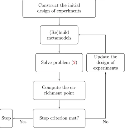
The main steps of SEGOMOE used in this paper are as follows:
1. Construct the initial DOE and build the associated MOE models relative to the objective and constraint functions.
2. Solve the optimization problem by maximizing the WB2 criterion subject to the design constraints and variable bounds, and propose the new enrichment point. In the original EGO algorithm,26 the mean and the variance of the objective function are required to compute the objective criterion (WB2). In our case, they are given in exactly the same way by the Kriging-based mixture of experts.
3. Compute the values of the objective and constraint functions at the new enrichment point.
4. Check if the new point is in the feasible domain or not, and identify inactive, active, and violated constraints.
5. Return to Step 2 and update the DOE if the stopping criterion is not reached.
SEGOMOE iterates until the stopping criterion is met. Due to the high computational cost of actual simulations, it is common to impose a maximum number of function calls as the stopping criterion. Finally, Figure2 summarizes the SEGOMOE algorithm steps.
Construct the initial design of experiments
(Re)build metamodels
Solve problem (2)
Compute the en-richment point
Stop criterion met? Stop
Update the design of experiments
Yes No
Figure 2. Overview of SEGOMOE algorithm.
In order to decrease the CPU time, two major improvements have been proposed concerning the updates of the surrogate models to build at each iteration step, their number has been reduced and their computation is done in parallel. At each iteration step, an identification of the active, respected and not-respected constraints is performed from the outputsci(x).
This selection is based on the distance between the constraint output (given by the solver) and the threshold value imposed by the user in order to check if the new point is in the feasible domain (or one of its boundaries) or not. Only the surrogate models relative to the objective function and to the active or not-respected constraints are updated taking into account the enriched database. Concerning the respected constraints, it is not useful to update their surrogate models at each iteration step of SEGOMOE but only after a fixed number of enrichment iterations (every 10 iterations by default if not specified by the user). Note that at each iteration step, the updates of the surrogate models relative to the objective function and the selected constraints can now be performed in parallel which is very powerful when a large number of constraints is involved.
SEGOMOE can easily be used as a global optimizer. The objective of the present paper is to illustrate its behaviour on two specific optimization problems. In the first problem, the objective function is unimodal (with a single global minimum), and the final solution obtained with a gradient-based optimizer such as SNOPT28or NLPQL29does not depend on the starting point. For the second problem, the objective function
is multimodal and thus we use a multistart approach to reach the global optimum with the gradient-based optimizer SNOPT. We describe these two test cases in the next sections and discuss the corresponding results.
III.
High-fidelity aerodynamic shape optimization framework
To demonstrate the capability of the SEGOMOE approach, we apply it to two aerodynamic shape optimization problems. To perform the aerodynamic shape optimization, we use a framework that combines
a Reynolds-averaged Navier–Stokes (RANS) CFD solver, a geometry parametrization engine, and a mesh perturbation algorithm. The CFD solver is ADflow, which uses a second-order finite-volume scheme to solve the compressible Euler equations, laminar Navier–Stokes, and RANS equations (steady, unsteady, and time periodic) on overset meshes.30,31 The Spalart–Allmaras turbulence model32 is used to complete the RANS
equations. The solver combines a Runge–Kutta method for the initial iterations with a Newton–Krylov algorithm that increases the convergence rate in the later iterations.
ADflow is especially effective when used in conjunction with gradient-based optimization because it ef-ficiently computes accurate gradients with respect to large numbers of design variables using an adjoint method. The adjoint method is implemented using a hybrid approach that selectively uses automatic differ-entiation to generate the code that computes the partial derivatives in the adjoint equations.31
The geometry is parametrized using an implementation of free-form deformation (FFD),33and the mesh
deformation is performed with an efficient analytic inverse distance method.34
The integration of ADflow with the optimization algorithms is achieved through pyOpt, a common Python interface that facilitates the use of different optimization algorithms.24,25 This enabled us to re-use the same Python scripts when benchmarking SEGOMOE against gradient-based optimizer. The gradient-based optimizers we used are SNOPT,28a sequential quadratic programming optimizer that can handle large-scale nonlinear constrained problems, and the Non-Linear Programming by Quadratic Lagrangian (NLPQL).29
This aerodynamic shape optimization framework has been used to solve various problems3,35–38 and has
also been extended to perform aerostructural design optimization.36,39–42
IV.
Twist optimization of the Common Research Model wing
A. Problem definition
As a first aerodynamic shape optimization problem, we solve a simplified version of the ADODG Case 4.9
This case consists in minimizing the drag coefficient of a wing by varying airfoil shapes and twist distributions subject to a lift coefficient constraint. The initial wing geometry is based on NASA’s Common Research Model (CRM) wing,3,43 which was created as a database for the purpose of validating specific applications
of CFD. The wing features a blunt trailing edge and is representative of a modern transonic commercial transport wing, with a size similar to that of a Boeing 777.
Since this case has been solved extensively using SNOPT,3,38 we decided to use this same case to bench-mark SEGOMOE using SNOPT as a reference. To limit the size of the optimization problem, we first remove the airfoil shape variables which leads to 8 variables (twist only). The optimization problem can be stated as,
min Drag coefficient, CD×104
w. r. t. 8 twist variables∈[−10,10] s. t. CL= 0.5
(4)
The 8 twist variables are given in degrees, and rotate the corresponding airfoil cross sections about the trailing edge. The trailing edge line is fixed. The angle-of-attack (AoA) is set at 2.8 degrees. The volume is constant with this formulation, since variations in twist do not change the wing thickness, so the volume constraint specified in the ADODG Case 4 does not need to be enforced. We only retain the lift coefficient constraint (CL= 0.5) from the original problem.
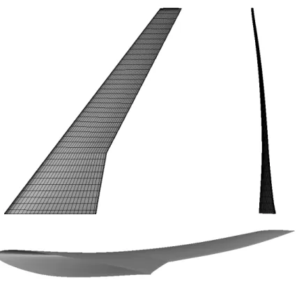
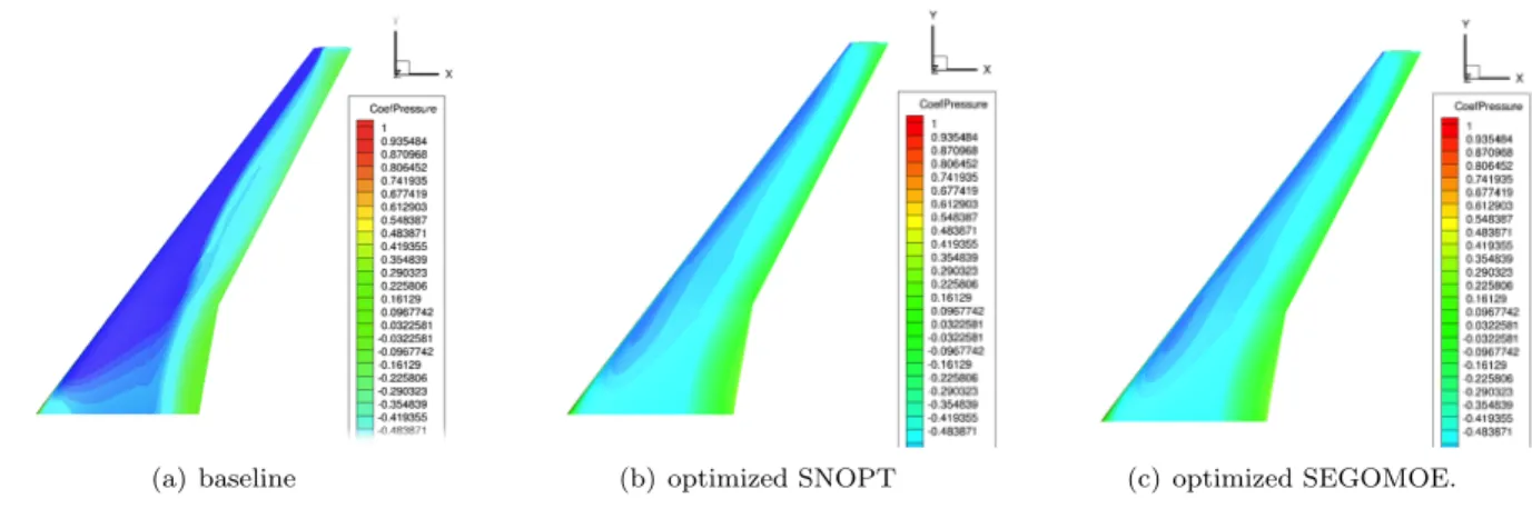
The baseline geometry of CRM wing is shown in Fig.3. This is identical to the CRM wing, except that all the twist variables are set to zero. We do this to verify that the optimizations are able to converge to the optimal twist distribution when starting far away from the optimal distribution. Figure7-a shows the CFD solution for this baseline at the nominal design flight condition. The solution shows a strong shockwave along the whole wing span that incurs a large drag penalty. This is not surprising because the CRM wing is designed to have decreasing twist towards the tip and this untwisted wing is far from optimal.
B. Results
The results obtained with SEGOMOE are compared with results obtained using the gradient-based op-timizers SNOPT and NLPQL. These gradient-based opop-timizers require an initial guess for the starting configuration and the derivatives of the objective function. On the other hand, SEGOMOE performs a DOE before allowing the optimizer to enrich the model, and therefore it does not need a starting point.
Figure 3. CRM baseline configuration used as starting point for gradient-based optimization.
The criterion chosen for comparison is the number of function calls required to minimize the drag coeffi-cient. SEGOMOE starts with a 9-point DOE (corresponding to the dimension of the design spaced+ 1) and the first step consists in finding a design point for which the constraints are satisfied. Then, the iterative process generates feasible points while reducing the objective function.
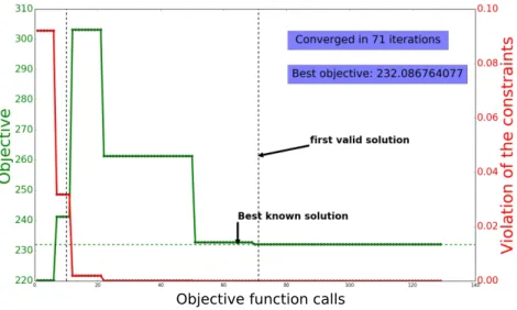
The results of the different steps are shown in Figs.4and5. The readers should notice that SEGOMOE optimization results are unconventional since they can be decomposed in an exploration phase (left part of the graph), then an exploitation phase (right part). These plot the objective values of the consecutive best points calculated throughout the optimization and the sum of the constraints violation. They also show the number of iterations required to converge, the value of the best calculated objective, and the number of iterations it took to find the first feasible point.
Two phases can be distinguished in these plots.
1. Before a first feasible point is found: This phase is characterized by a nonzero sum of the violation of the constraints (red line). During this phase, the consecutive best points are the ones that make this sum decrease. Hence, the objective function of the consecutive best points is not necessarily decreasing, and can have a lower value than the final best found point.
2. After the first feasible point is found: This phase is characterized by a sum of the violation of the constraints that remains zero and a decreasing objective function. The two phases are separated by a dotted vertical line with the label “first valid solution”.
As seen in Figs. 4 and 5, the optimizer is not deterministic, that is, two consecutive runs of the same optimization under the exact same circumstances do not yield the exact same results, or at least they do not have the same DOE and enrichment points. In this example, COBYLA algorithm with a multistart procedure is used to maximize the WB2 enrichment criterion given by Eq. (2). Although the convergence histories look very different, the two best objective values are very similar (10−4 relative error) and the
optimizations converged using a similar number of objective function calls.
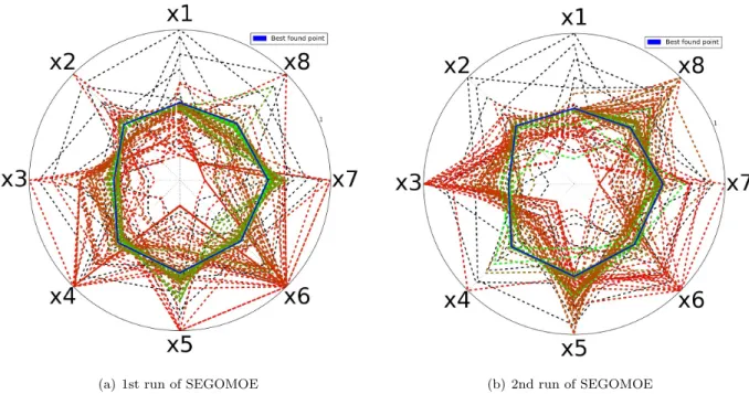
Now let’s have a look to how the optimizer explores the design space over iteration steps. We propose to represent the design space using a radar chart, where each direction of this chart represents a design variable. Figure6displays the radar chart for the optimization with 8 twist design variables (x1, x2, . . . , x8).
Objective function calls
Figure 4. Optimization convergence history using SEGOMOE and a 9-point DOE (Run 1). The best points are displayed in green, and the sum of the constraint violations is displayed in red (which is zero when a feasible point is found). Before the first feasible solution is found, the best points are those for which the sum of the constraints violation is smaller than the previous one.
Objective function calls
Figure 5. Optimization convergence history using SEGOMOE and a 9-point DOE (Run 2). The best points are displayed in green, the sum of the constraint violations is displayed in red (zero for feasible points). Before the first feasible solution is found, the best points are those for which the sum of the constraints violation is smaller than the previous one.
The DOE points are represented with black dotted lines. The iteration steps (timeline) of the enrichment points is represented by coloring the corresponding lines from red to green. Finally, the best found point is represented by a solid blue line.
As can be seen on Fig. 6, the optimizer explored the design space in very distinct ways, and spent some time looking for the optimum in different areas. However, the best points found are the same and this was the case for every SEGOMOE run. Therefore, we can conclude that the final results are consistent despite variations in the optimization history.
The results presented above are consistent, but they provide no information about the quality of the optimum that it found. To assess the quality of the optimal design, we then compare to the optimum found
(a) 1st run of SEGOMOE (b) 2nd run of SEGOMOE
Figure 6. Radar charts for the two SEGOMOE optimizations (Run 1 and 2), using COBYLA algorithm to max-imize the WB2 criterion. The timeline of the enrichment process is represented by coloring the corresponding lines from red to green. The blue line represents the best design found.
with SNOPT.
Table1summarizes the performance of SNOPT, NLPQL and SEGOMOE for the CRM twist optimization case. To get a final value close to the reference one (with a relative error of 10−6 compared to the SNOPT
value), SEGOMOE requires a few more evaluations (about 20) than SNOPT, but again no initial starting point is required. To get a relative error of 10−3, SEGOMOE requires fewer iterations (about 30, depending
on the run) than SNOPT. This behavior is due to one of SEGOMOE’s skills: smart exploration of the domain to propose rapidly a solution near the global optimum. Once again, we emphasize the fact that SEGOMOE does not need the objective or constraint derivatives, or a starting point. However, SEGOMOE can be adapted to use derivatives by using a gradient-enhanced kriging technique.44 Also, the results and computational cost of both SNOPT and NLPQL are dependent on the starting point, and the search for a suitable starting point can sometimes be time consuming for complex cases.
Optimization run Number of calls Best objective
SNOPT 97 232.0884
NLPQL 103 232.0993
SEGOMOE run 1 119 (10−6rel. error) 69 (10−3 rel. error) 232.0867
SEGOMOE run 2 114 (10−6rel. error) 71 (10−3 rel. error) 232.0884
Table 1. Performance of the various optimizers for the 8-variable twist optimization problem. The reference objective value is the SNOPT result shown in bold and is used to compute the relative error. The number of calls for gradient-based optimizers (SNOPT and NLPQL) include adjoint computation.
As illustrated on Fig. 7, the pressure distribution over the optimized wing is much smoother and does not have a shockwave anymore. The optimized shapes obtained by SNOPT and SEGOMOE are very close and lead to the same pressure distributions.
(a) baseline (b) optimized SNOPT (c) optimized SEGOMOE. Figure 7. Comparison of the surface pressure distributions on the CRM wing: baseline wing for SNOPT (left), wing optimized with SNOPT (middle), wing optimized with SEGOMOE (right).
V.
Multimodal wing shape optimization
A. Problem definition
This new test case is based on the ADODG Case 6 benchmark (“Multimodal Subsonic Inviscid Optimiza-tion”).9,45 This case was devised to explore the existence of multiple local minima in aerodynamic wing
design. The baseline geometry is a rectangular wing with a chord of 1.0 m and a NACA 0012 airfoil cross-section with a sharp trailing edge. The semispan is 3.06 m and the wing is fitted with a rounded wingtip cap. In the full benchmark problem, the optimizer is given freedom to change twist, chord, dihedral, sweep, span, and sectional shape variables. In the modified version used for this study, we reduced the variables to twist and dihedral. The geometry is parameterized using the FFD approach implemented in pyGeo,33
which allows the definition of global design variables with control of sections of B-spline control points. Nine sections are defined along the span of the wing with heavier clustering towards the tip of the wing. Twist variables rotate eight of these sections (excluding the root section) about the quarter-chord. Likewise, the eight dihedral variables each control the vertical displacement of one of the spanwise sections, excluding the root section. The angle of attack can be varied to allow the optimizer to satisfy the lift constraint. The optimization problem we solve is
min drag coefficient: CD×104
w. r. t. 8 twist variables∈[−3.12,3.12] 8 dihedral variables ∈[−0.25,0.25] 1 angle-of-attack ∈[−3.0,6.0] s. t. CL= 0.2625 (5) B. Results
We used two optimization approaches to obtain the results in this section.
SEGOMOE : This consists in using solely SEGOMOE as a global optimizer to assess its performance in terms of ability to find the global optimum within a limited budget (i.e., number of calls to the CFD solver).
Hybrid : In this approach, we use SEGOMOE as a first exploration stage and then switch to a gradient-based optimizer, such as SNOPT. The idea is to quickly identify a design that is close to the global minimum, and then use a gradient-based algorithm to precisely converge to that minimum.
1. SEGOMOE-only results
As for the previous use case on CRM wing, the SEGOMOE approach is compared to SNOPT on the same test case. These gradient-based results, as well as other cases related to ADODG Case 6, are presented in
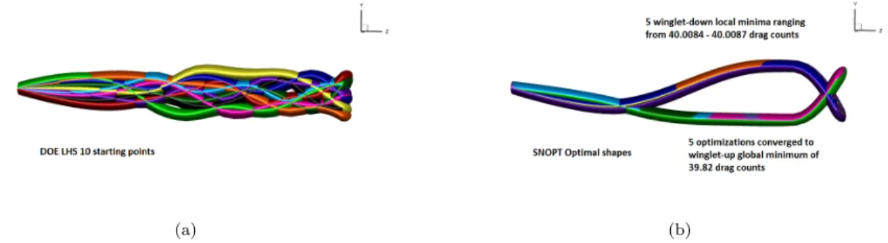
more detail by Bons et al.45 Here we just compare the SEGOMOE results for the Euler-based twist and dihedral optimization case, and summarize the corresponding results from Bons et al.45 for completeness. The optimization problem was solved using SNOPT28 starting from 10 random shapes, as illustrated in
Fig.8-a.
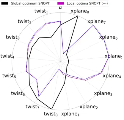
The optimal results are shown on Fig.8-b. It appears that this problem does have multiple local optima and a single global one, although the designs are very close in terms of drag value: 39.820 drag counts for the global optimum and 40.001 drag counts for the local one. Of the 10 runs, 5 converged towards the global optimum, which is characterized by an upward winglet. For the 5 other runs, multiple local minima were found for shapes with a downward winglet. The radar chart in Fig.9 provides more details on the optimal designs with the values of the 17 design variables; we can see that all local minima differ only slightly on twist parameters and on dihedral parameters in the inner part of the wing (the dihedral variables are denoted as “xplane”).
(a) (b)
Figure 8. SNOPT results for wing optimization with respect to twist and dihedral variables. Multiple local minima were found when starting from 10 randomly generated initial configurations.
All the computations converged to a constraint violation below 10−8(10−11for some runs) for the equality
constraint, resulting in an average number of iterations around 100, corresponding to 200 calls to the ADflow solver (which requires an adjoint computation in addition to the flow solution). Table 2 summarizes the reference target, in terms of best objective and computational budget achieved by the SNOPT algorithm.
Optimizer Best objective Number of calls Constraint violation SNOPT 39.820 Mean≈200 ≈10−09–10−11
min= 180; max =220
Table 2. Result achieved by SNOPT for a 200 function call budget, where the number of calls is the average of 5 runs. The min and the max value of the ADFlow calls for the 5 runs are also reported.
A set of SEGOMOE computations was launched to benchmark its performance for a budget similar to that of an average SNOPT optimization (200 calls to the CFD solver), and also to assess the robustness of the approach. With that goal in mind, two different DOE sizes were tested:
• 3 runs for an initial 18-point DOE
• 3 runs for an initial 30-point DOE
Table3summarizes the performance of all SEGOMOE runs. These results should be compared with reference value given in Table2. These results show that, within the available budget, all SEGOMOE runs reached objective value close to the optimal one with a constraint violation between 10−7 and 10−10. The lowest
values of objective function with SEGOMOE are reached by the optimization using an initial DOE size of 30. Nevertheless, among the runs that use the smaller initial DOE (18 points), one point is more interesting to study as its objective value is 39.833 and its equality constraint is satisfied with a tolerance of 9.78 10−08
(which is very close to the reference one obtained with SNOPT).
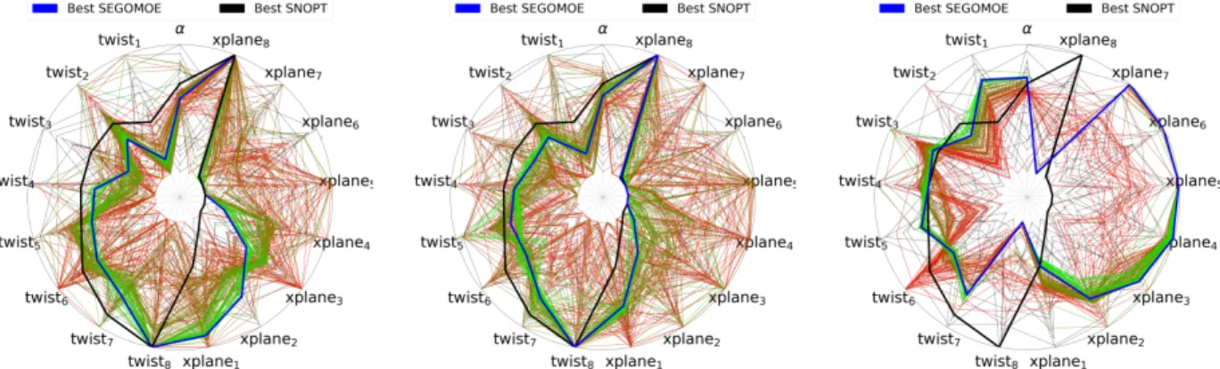
Figure10shows the radar charts for the best configurations from the 6 trials listed in Table3. The global minimum obtained by SNOPT is shown in each plot in black. None of the optimizations reached the global optimum shape, but most of them converge to a point nearby. Of the 6 resulting shapes, 5 converged to an upward winglet as the configuration providing the best result. For the runs starting from a 18-point DOE,
Figure 9. Reference optimal designs obtained using the SNOPT optimizer (multistart of 10 random configu-rations). Each direction of the radar chart represents one of the 17 design variables (“twist” refers to twist variables and “xplane” refers to dihedral variables), with the inner and outer radii limiting the design space. The continuous black line refers to the the global optimum in the design space. The dashed lines (magenta or blue) refer to the local optimal points.
Reference objective value given by SNOPT:39.820
SEGOMOE run number Initial DOEs Best objective Number of calls Constraint violation 1 18 39.941 197 (18+179) 1.82×10⁻⁷ 2 18 39.859 174 (18+156) 4.49×10⁻¹⁰ 3 18 40.038 184 (18+166) 9.95×10⁻⁹ 1 30 39.848 167 (30+137) 4.74×10⁻⁸ 2 30 39.833 198 (30+168) 9.78×10⁻⁸ 3 30 39.867 194 (30+164) 9.62×10⁻⁸
Table 3. SEGOMOE results, where the number of calls includes both the DOE sampling and optimization iterations. Comparisons are made with two different DOE sizes for a fixed budget of 200 calls to the solver. The reference value form SNOPT and the best objective value with SEGOMOE are given in bold
.
runs 1 and 2 found the same area of the design space, which was close to the SNOPT reference. On the other hand, run 3 identified the design space where the local minima found by SNOPT are located. The shape discrepancies between run 1, run 2, and the local exploration done by run 3, indicate that the convergence was not achieved by these runs. One would expect that with more iterations, run 3 of SEGOMOE could change its current exploration area to the one identified by the other runs and achieve a lower objective function value and lower constraint violation. For the three runs starting from the larger 30-point DOE, the global minimum region is successfully found in all trials. The final shapes seem closer to one another, and both objective value and constraint violation are within a limited range. According to these results, a larger DOE size is more efficient for this case when the budget of calls forces a premature termination.
(a) 1st run SEGOMOE with 18-point DOE
(b) 2nd run SEGOMOE with 18-point DOE
(c) 3rd run SEGOMOE with 18-point DOE
(d) 1st run SEGOMOE with 30-point DOE
(e) 2nd run SEGOMOE with 30-point DOE
(f) 3rd run SEGOMOE with 30-point DOE
Figure 10. Radar charts for the six SEGOMOE optimizations (18- and 30-point initial DOE, for three different runs). Each direction of the chart represents one of the 17 design variables, with the inner and outer radii limiting the design space. The timeline of the enrichment process is represented by coloring the corresponding lines from red to green. The blue line is the best found point from SEGOMOE and the black one is the reference SNOPT optimal design.
Figures 11and12show the geometry for each of the six configurations compared to the SNOPT global optimum. These are consistent with the radar chart presented above, and we conclude that:
• For the SEGOMOE optimizations based on a DOE of 18 points, the run 3 best configuration (pink) is located in a local minimum area (see Fig. 8), whereas the two other runs (red and blue) exhibit a positive dihedral shape.
• For the SEGOMOE optimizations based on a DOE of 30 points, the three runs get closer to the global optimal shape; the best configuration identified by SEGOMOE is shown in blue.
These investigations confirm SEGOMOE’s global exploration capabilities, since 5 out of 6 computations find the global optimum area in a limited budget.
2. Hybrid approach: SEGOMOE followed by SNOPT
Based on the results above, we decided to take the best of both worlds and combine SEGOMOE and SNOPT in a hybrid approach. The idea is to use SEGOMOE as a first exploration stage and then use SNOPT starting from the SEGOMOE best point from the first stage. For this study, two different starting points were extracted from previous SEGOMOE optimization runs. The best wings obtained after a fixed budget of 100 calls were selected from the two best SEGOMOE combinations of options identified in the previous paragraph—namely, SEGOMOE 30 run 1, and SEGOMOE 30 run 2. Figure13 shows the radar
(a) 3D view of best configurations (b) Side view of best configurations
Figure 11. Comparison of SEGOMOE best wing shapes obtained from an initial 18-point DOE with SNOPT global optimum.
(a) 3D view of best configurations (b) Side view of best configurations
Figure 12. Comparison of SEGOMOE best wing shapes obtained from an initial 30-point DOE with SNOPT global optimum.
chart of the two retained initial configurations. We can see that even with a limited budget in terms of CFD calls, the wings are already close to the best shape of each run and are in the vicinity of the global optimum given by SNOPT.
(a) 1st run (b) 2nd run
Figure 13. Radar charts corresponding to two best configurations obtained with SEGOMOE with a 30-point DOE and a maximum budget of 100 calls.
After the exploration stage performed by SEGOMOE, the exploitation is done with SNOPT in two optimizations starting from the two best designs found by SEGOMOE. The performance of the hybrid approach is compared to SNOPT-only results in Table4.
SEGOMOE SEGOMOE SNOPT calls SNOPT Constraint Total ADflow starting point calls (including adjoint) Objective violation calls 30-point DOE, run 1 100 129 (65+64) 39.820 4.42×10⁻⁹ 229
30-point DOE, run 2 100 123 (62+61) 39.820 −5.68×10⁻⁹ 223
Table 4. SNOPT results starting from two different SEGOMOE selected designs.
As expected, both SNOPT optimizations converged towards the global optimum that we had already identified, using about 60 iterations. In this hybrid approach, the metric to be considered is the total number of calls to the CFD solver (including the adjoint computations), which are listed in Table4. For the cases considered, the total number of calls of the hybrid approach is ranged from 220 to 230, compared to an average of 200 for the SNOPT-only approach. However, recall that only 5 out 10 SNOPT runs converged towards the global optimum, whereas, with the hybrid approach, we can run the procedure only once and ensure convergence to the global optimum. To assess the robustness of this hybrid approach, more numerical experiments should be performed to check if using a well-chosen starting point from SEGOMOE ensures the SNOPT convergence towards the global minimum. A compromise between the allocated budget for SEGOMOE and for SNOPT should also be investigated to reduce the total number of calls and achieve a fast and reliable optimization strategy.
VI.
Conclusion
In order to create a breakthrough in aircraft design, researchers need to integrate more accurate data from computer simulation of higher fidelity at the very beginning of the design process. Thus we have developed an original method so called SEGOMOE to obtain optimized configurations at a reasonable computational cost. This approach can tackle complex design optimization problems through the use of an adaptive surrogate modeling approach based on Kriging. The results prove that SEGOMOE is a promising algorithm for solving expensive high-dimensional constrained optimization. The first test case (wing aerodynamic shape optimization case with 8 design variables) demonstrated the efficiency of our approach in locating the global minimum using a limited number of function calls. Then we also propose a second set of results using the ADODG Case 6 benchmark to identify the different local minima. SEGOMOE succeed in obtaining fast and reliable solution. Within a similar budget of function calls, the optimal global minimum was found to be very close from the SNOPT reference solution. SEGOMOE seems very interesting for locating the global minima zone under constrained budget. Further works will focus on adding the multi-point approach46 for
the EI enrichment process and thus perform parallel computations.
Finally the proposed hybrid approach can combine the advantages of SEGOMOE and SNOPT method. SEGOMOE is capable of locating the global optimum area very quickly. SNOPT excels in finding the best solution when its starting point is in the general vicinity of the global optimum. From those conclusions, when it is possible, i.e., when objective function derivatives are available, the best optimization strategy is to let SEGOMOE find a good starting point for SNOPT. The preliminary results for this hybrid approach show a total number of function calls similar to the SNOPT-only optimization. This new approach could be well adapted to industrial needs requiring fast and reliable optimization, especially for innovation in aircraft design where researchers want to use optimizers capable of large exploration of the design space.
VII.
Acknowledgments
We would like to thank the following internship students for their work on the SEGOMOE optimizer: R´emy Priem, Vivien Stilz, Marie Gibert, and Valentin Fievez. We are also grateful to R´emi Lafage for his support with the SEGOMOE framework and the ADflow installation at ONERA. This work was supported by the AGILE project (Aircraft 3rd Generation MDO for Innovative Collaboration of Heterogeneous Teams of Experts) and has received funding from the European Union Horizon 2020 Program (H2020-MG-2014-2015) under grant agreement no636202. Additional support was provided by the Air Force Office of Scientific
Research (AFOSR) MURI on “Managing multiple information sources of multi-physics systems,” Program Officer Jean–Luc Cambier, Award Number FA9550-15-1-0038.
References
1“Clean Sky project,”http://www.cleansky.eu/.
2Jones, D., “Large-scale multi-disciplinary mass optimization in the auto industry,”MOPTA 2008 Conference (20 August
2008), 2008.
3Lyu, Z., Kenway, G. K., and Martins, J. R., “Aerodynamic Shape Optimization Investigations of the Common Research Model Wing Benchmark,”AIAA Journal, Vol. 53, No. 4, 2014, pp. 968–985.
4Sasena, M. J., Papalambros, P. Y., and Goovaerts, P., “The Use of Surrogate Modeling Algorithms to Exploit Disparities in Function Computation Time Within Simulation-Based Optimization,” In the Fourth World Congress of Structural and Multidisciplinary Optimization, 2001, pp. 1–6.
5Bouhlel, M. A., Bartoli, N., Otsmane, A., and Morlier, J., “Improving kriging surrogates of high-dimensional design models by Partial Least Squares dimension reduction,”Structural and Multidisciplinary Optimization, Vol. 53, No. 5, 2016, pp. 935–952.
6Bouhlel, M. A., Bartoli, N., Otsmane, A., and Morlier, J., “An Improved Approach for Estimating the Hyperparameters of the Kriging Model for High-Dimensional Problems through the Partial Least Squares Method,”Mathematical Problems in Engineering, Vol. 2016, 2016.
7Bartoli, N., Kurek, I., Lafage, R., Lefebvre, T., Priem, R., Bouhlel, M.-A., Morller, J., Stilz, V., and Regis, R., “Improve-ment of efficient global optimization with mixture of experts: methodology develop“Improve-ments and preliminary results in aircraft wing design,”17th AIAA/ISSMO Multidisciplinary Analysis and Optimization Conference, Washington D.C., USA, June 2016 2016.
8Heath, C. M. and Gray, J. S., “OpenMDAO: Framework for Flexible Multidisciplinary Design, Analysis and Optimization Methods,”8th AIAA Multidisciplinary Design Optimization Specialist Conference (MDO), Honolulu, Hawaii, 2012, pp. 1–13. 9“Aerodynamic Design Optimization DG,”https://info.aiaa.org/tac/ASG/APATC/AeroDesignOpt-DG/default.aspx. 10Forrester, A. I. and Keane, A. J., “Recent advances in surrogate-based optimization,”Progress in Aerospace Sciences, Vol. 45, No. 1, 2009, pp. 50–79.
11Matheron, G., “Principles of geostatistics,”Economic geology, Vol. 58, No. 8, 1963, pp. 1246–1266.
12Sacks, J., Welch, W. J., Mitchell, T. J., and Wynn, H. P., “Design and analysis of computer experiments,”Statistical
science, 1989, pp. 409–423.
13Wold, H., “Soft modeling by latent variables: the nonlinear iterative partial least squares approach,” Perspectives in
probability and statistics, papers in honour of MS Bartlett, 1975, pp. 520–540.
14University of Michigan, ONERA, and ISAE-SUPAERO, “Surrogate Model Toolbox,”https://github.com/SMTorg/SMT/. 15Hastie, T., Tibshirani, R., Friedman, J., and Franklin, J., “The elements of statistical learning: data mining, inference and prediction,”The Mathematical Intelligencer, Vol. 27, No. 2, 2005, pp. 83–85.
16Jordan, M. I. and Jacobs, R. A., “Hierarchical mixtures of experts and the EM algorithm,”Neural computation, Vol. 6, No. 2, 1994, pp. 181–214.
17Bettebghor, D., Bartoli, N., Grihon, S., Morlier, J., and Samuelides, M., “Surrogate modeling approximation using a mixture of experts based on EM joint estimation,” Structural and Multidisciplinary Optimization, Vol. 43, No. 2, 2011, pp. 243–259, 10.1007/s00158-010-0554-2.
18Liem, R. P., Mader, C. A., and Martins, J. R. R. A., “Surrogate Models and Mixtures of Experts in Aerodynamic Performance Prediction for Mission Analysis,”Aerospace Science and Technology, Vol. 43, 2015, pp. 126–151.
19Pedregosa, F., Varoquaux, G., Gramfort, A., Michel, V., Thirion, B., Grisel, O., Blondel, M., Prettenhofer, P., Weiss, R., Dubourg, V., Vanderplas, J., Passos, A., Cournapeau, D., Brucher, M., Perrot, M., and Duchesnay, E., “Scikit-learn: Machine Learning in Python,”Journal of Machine Learning Research, Vol. 12, 2011, pp. 2825–2830.
20Watson, A. G. and Barnes, R. J., “Infill sampling criteria to locate extremes,”Mathematical Geology, Vol. 27, No. 5, 1995, pp. 589–608.
21Powell, M. J., “A direct search optimization method that models the objective and constraint functions by linear inter-polation,”Advances in optimization and numerical analysis, Springer, 1994, pp. 51–67.
22Kraft, D. et al.,A software package for sequential quadratic programming, DFVLR Obersfaffeuhofen, Germany, 1988. 23Jones, E., Oliphant, T., Peterson, P., et al., “SciPy: Open source scientific tools for Python,” 2001–, [Online; accessed 2016-04-27].
24Perez, R. E., Jansen, P. W., and Martins, J. R. R. A., “pyOpt: A Python-Based Object-Oriented Framework for Nonlinear Constrained Optimization,”Structures and Multidisciplinary Optimization, Vol. 45, No. 1, 2012, pp. 101–118.
25Kenway, G. K. W., “pyOptSparse - PYthon OPTimization (Sparse) Framework,” 2014,https://bitbucket.org/mdolab/
pyoptsparse.
26Jones, D. R., Schonlau, M., and Welch, W. J., “Efficient global optimization of expensive black-box functions,”Journal
of Global optimization, Vol. 13, No. 4, 1998, pp. 455–492.
27Sasena, M.,Flexibility and efficiency enhancements for constrained global design optimization with Kriging
approxima-tions, Ph.D. thesis, University of Michigan, 2002.
28Gill, P. E., Murray, W., and Saunders, M. A., “SNOPT: An SQP algorithm for large-scale constrained optimization,”
SIAM review, Vol. 47, No. 1, 2005, pp. 99–131.
29Schittkowski, K., “NLPQL: A FORTRAN subroutine solving constrained nonlinear programming problems,”Annals of
operations research, Vol. 5, No. 2, 1986, pp. 485–500.
30Kenway, G. K. W., Secco, N., Martins, J. R. R. A., Mishra, A., and Duraisamy, K., “An Efficient Parallel Overset Method for Aerodynamic Shape Optimization,”Proceedings of the 58th AIAA/ASCE/AHS/ASC Structures, Structural Dynamics, and Materials Conference, AIAA SciTech Forum, Grapevine, TX, January 2017.
31Lyu, Z., Kenway, G. K. W., Paige, C., and Martins, J. R. R. A., “Automatic Differentiation Adjoint of the Reynolds-Averaged Navier-Stokes Equations with a Turbulence Model,”43rd AIAA Fluid Dynamics Conference and Exhibit, June 2013, AIAA 2013-2581.
32SPALART, P. and ALLMARAS, S., “A one-equation turbulence model for aerodynamic flows,”30th Aerospace Sciences
Meeting and Exhibit, Aerospace Sciences Meetings, American Institute of Aeronautics and Astronautics, jan 1992.
33Kenway, G. K., Kennedy, G. J., and Martins, J. R. R. A., “A CAD-Free Approach to High-Fidelity Aerostructural Optimization,”Proceedings of the 13th AIAA/ISSMO Multidisciplinary Analysis Optimization Conference, Fort Worth, TX, Sept. 2010, AIAA 2010-9231.
34Luke, E., Collins, E., and Blades, E., “A Fast Mesh Deformation Method Using Explicit Interpolation,” Journal of
Computational Physics, Vol. 231, No. 2, Jan. 2012, pp. 586–601.
35Kenway, G. K. W. and Martins, J. R. R. A., “Buffet Onset Constraint Formulation for Aerodynamic Shape Optimization,”
AIAA Journal, 2017, (In press).
36Liem, R. P., Martins, J. R. R. A., and Kenway, G. K., “Expected Drag Minimization for Aerodynamic Design Optimization Based on Aircraft Operational Data,”Aerospace Science and Technology, Vol. 63, April 2017, pp. 344–362.
37Chen, S., Lyu, Z., Kenway, G. K. W., and Martins, J. R. R. A., “Aerodynamic Shape Optimization of the Common Research Model Wing-Body-Tail Configuration,”Journal of Aircraft, Vol. 53, No. 1, January 2016, pp. 276–293.
38Kenway, G. K. W. and Martins, J. R. R. A., “Multipoint Aerodynamic Shape Optimization Investigations of the Common Research Model Wing,”AIAA Journal, Vol. 54, No. 1, January 2016, pp. 113–128.
39Kenway, G. K. W., Kennedy, G. J., and Martins, J. R. R. A., “Scalable Parallel Approach for High-Fidelity Steady-State Aeroelastic Analysis and Derivative Computations,”AIAA Journal, Vol. 52, No. 5, May 2014, pp. 935–951.
40Kenway, G. K. W. and Martins, J. R. R. A., “Multipoint High-Fidelity Aerostructural Optimization of a Transport Aircraft Configuration,”Journal of Aircraft, Vol. 51, No. 1, January 2014, pp. 144–160.
41Brooks, T. R., Kennedy, G. J., and Martins, J. R. R. A., “High-fidelity Multipoint Aerostructural Optimization of a High Aspect Ratio Tow-steered Composite Wing,” Proceedings of the 58th AIAA/ASCE/AHS/ASC Structures, Structural Dynamics, and Materials Conference, AIAA SciTech Forum, Grapevine, TX, January 2017.
42Burdette, D. A., Kenway, G. K., and Martins, J. R. R. A., “Performance Evaluation of a Morphing Trailing Edge Using Multipoint Aerostructural Design Optimization,”57th AIAA/ASCE/AHS/ASC Structures, Structural Dynamics, and Materials Conference, American Institute of Aeronautics and Astronautics, January 2016.
43Vassberg, J. C., DeHaan, M. A., Rivers, S. M., and Wahls, R. A., “Development of a common research model for applied CFD validation studies,”AIAA paper, Vol. 6919, 2008, pp. 2008.
44Mortished, C., Ollar, J., Jones, R., Benzie, P., Toropov, V., and Sienz, J., “Aircraft Wing Optimisation based on Computationally Efficient Gradient-Enhanced Kriging,”57th AIAA/ASCE/AHS/ASC Structures, Structural Dynamics, and Materials Conference San Diego, California, USA, 2016.
45Bons, N. P., He, X., Kenway, G. K. W., and Martins, J. R. R. A., “Multimodality in Aerodynamic Wing Design Optimization,” 18th AIAA/ISSMO Multidisciplinary Analysis and Optimization Conference, Denver, Colorado, USA, June 2016 2017.
46Chevalier, C.,Fast uncertainty reduction strategies relying on Gaussian process models, Theses, Universit¨at Bern, Sept. 2013.
![Figure 1. The EGO enrichment for a black box function (1D function f (x) = (6x − 2) 2 sin(12x − 4), x ∈ [0, 1]) with the EI and WB2 criteria](https://thumb-us.123doks.com/thumbv2/123dok_us/1882645.2774814/4.918.112.811.534.729/figure-ego-enrichment-black-box-function-function-criteria.webp)