An Approach to Solving Large-Scale
SLAM Problems with a Small Memory Footprint
Benjamin Suger
Gian Diego Tipaldi
Luciano Spinello
Wolfram Burgard
Abstract—In the past, highly effective solutions to the SLAM problem based on solving nonlinear optimization problems have been developed. However, most approaches put their major focus on runtime and accuracy rather than on memory consumption, which becomes especially relevant when large-scale SLAM problems have to be solved. In this paper, we consider the SLAM problem from the point of view of memory consumption and present a novel approximate approach to SLAM with low memory consumption. Our approach achieves this based on a hierarchical decomposition consisting of small submaps with limited size. We perform extensive experiments on synthetic and publicly available datasets. The results demonstrate that in situations in which the representation of the complete map requires more than the available main memory, our approach, in comparison to state-of-the-art exact solvers, reduces the memory consumption and the runtime up to a factor of 2 while still providing highly accurate maps.
I. INTRODUCTION
Map building and SLAM is one of the fundamental problems in mobile robotics as being able to learn what the environment looks like is typically regarded as a key prerequisite to truly autonomous mobile systems. In the past highly effective SLAM methods have been developed and state-of-the-art SLAM solvers are able to achieve accurate solutions in a minimum amount of time [20, 12, 6]. In this paper we look at the SLAM problem from an additional perspective and seek for a SLAM solver that can quickly produce accurate solutions while also being efficient with respect to the memory consumption. We regard this aspect as particularly relevant when one has to solve large-scale SLAM problems or for memory-restricted systems. In the case of large mapping problems, an algorithm that is not designed to be memory efficient will eventually try to allocate more than the available main memory on the computer. This typically triggers paging mechanisms of the operating system, during which parts of the memory are stored to or retrieved from the hard disk, thus largely slowing down the execution. We are convinced that the memory efficiency is highly relevant for the development of low-cost robotic systems where hardware resources are often extremely limited to be competitive on the consumer market.
Due to the robustness of approaches to robot navigation and SLAM, the range of autonomous navigation for robots is rapidly increasing. City-scale autonomous navigation [16] is already possible and autonomous cars have travelled hundreds of kilometers through the desert [24] and navigated for hours
All authors are with the University of Freiburg, Institute of Computer Science, 79110 Freiburg, Germany. This work has partly been supported by the European Commission under the grant no. ERC-AG-PE7-267686.
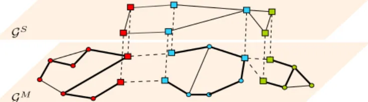
Fig. 1. The proposed small memory footprint approach is based on a hierarchical graph partition. In each partitionGM
i (same color) we identify
separator nodesVS(squares) and interior nodesVM(circles). This implicitely
partitions the edges into separator edgesES(dashed lines) and interior edges
EM (solid lines). We build the graph of the separator nodes inGS by using
a tree approximation on each subgraph (thick lines). We optimize on each layer and on disjoint subgraphs, from bottom to top and vice versa. With our algorithm, we never optimize the entire graph as a whole.
in city-like traffic environments [25]. There are several modern techniques that address the problem of learning large-scale maps required by such applications [1, 3, 7, 19]. However, these approaches mostly concentrate on accuracy and runtime and the memory consumption has not been their major focus. In this paper we present a novel algorithm that is able to solve large mapping problems with low memory consumption. Our method employs adivide-and-conquer principle to hierar-chically subdivide the problem in many submaps of small size with limited dependencies and to solve a fine-to-coarse followed by a coarse-to-fine least-squares map optimization. At each level of the hierarchy, we subdivide the graph into subgraphs. We optimize each subgraph independently from the others and approximate it coarsely (fine-to-coarse approximation). All the approximated subgraphs, along with the edges that connect them, constitute the graph at the next level. We iterate this process until we reach a desired top level. Then, we carry out coarse-to-fine map adjustments by traversing the hierarchy in a top-down manner and performing an optimization at each level. Our algorithm does not require a specific graph clustering technique. Rather, every technique that is able to limit the number of nodes per cluster constitutes a valid choice. We present extensive experiments in which we evaluate metric accuracy, memory footprint and computation time. The results obtained by running the methods on publicly available datasets demonstrate that our approach yields a precision that compares to that of other state-of-the-art methods. In addition, we perform evaluations on large-scale datasets consisting of hundreds of thousands of nodes and demonstrate that our method exhibits lower memory consumption than the state-of-the-art implementations. For memory-constrained systems,
for which the entire data do not fit into main memory, our approach is able to solve problems 2 times faster.
II. RELATEDWORK
Over the past years, SLAM has been an enormously active research area and a variety of approaches to solve the SLAM problem has been presented. More recently, optimization meth-ods applied to graph-based SLAM formulations have become popular. Lu and Milios [17] were the first to refine a map by globally optimizing the corresponding system of equations to reduce the error introduced by constraints. Subsequently, Gutmann and Konolige [9] proposed a system for constructing graphs and for detecting loop closures incrementally. Since then, several approaches for minimizing the error in the constraint network have been proposed, including relaxation methods [10, 4], stochastic gradient descent [20] and similar variants [6] as well as smoothing techniques [12]. In a recent approach, Kaesset al. [11] provide an incremental solution to the SLAM problem that relies on Bayes Trees.
Closely related to our work presented here are hierarchical SLAM methods. And several of them perform the optimization on multiple hierarchies. For example, the ATLAS framework [1] constructs a two-level hierarchy combining a Kalman filter and global optimization. Estrada et al.proposed Hierarchical SLAM [3] as a technique for using independent local maps, which they merge when the robot re-visits a place. Frese [5] proposed an efficient strategy to subdivide the map in a tree of subregions. In the case of an unbalanced tree and when the leaves contain many poses, his method suffers from high computational demands. HogMan [7] builds up a multi-layer pose-graph and employs a lazy optimization scheme for online processing. The hierarchy generated is always fixed and is based on special decimation principles. One can modify HogMan so as to address low-memory situations at the price of performing optimization only on levels that can be loaded in memory. A divide and conquer approach has been presented by Ni
et al. in [18], who divide the map into submaps, which are independently optimized and eventually aligned. This method was later extended by Ni et al. [19], which turns out to be the closest approach with respect to technique presented here. They employ nested dissection to decompose the graph in a multi-level hierarchy by finding node separators and perform inference with the cluster tree algorithm.
Kretzschmar et al.[14], apply graph compression using an efficient information-theoretic graph pruning strategy. They build a constant size map by actively removing nodes in the map. After pruning them away, their information can not be recovered any longer. In contrast with them, our method stores all the information in the hierarchy. In a visual SLAM context, Strasdat et al.[23] presented a double window optimization approach. They perform local bundle adjustment (inner window) and approximate pose-graph minimization (outer window). They reduce the complexity of full map optimization but do not bound the size of the outer window. Our approach can be seen as a multiple window optimization, where each window is one level of the hierarchy. Lately, a similar approach to
approximating subgraphs with tree-like subgraphs has been independently proposed by Grisetti et al.[8]. The condense
local submaps in a set of virtual measurements to improve the initial estimate for a non-linear minimization algorithm on the whole graph. Note that the aim of our work is different: we aim to provide an accurate and efficient solution to large-scale SLAM problems in situations in which the entire map does not fit into main memory.
III. MAPPING WITHLOWMEMORYCONSUMPTION In this paper we consider the SLAM problem in its probabilistic graph-based interpretation. Letx= [x1, . . . ,xn]T be the vector of robot poses, wherexiis the pose of the robot at timei. Letzij andΩijbe the mean and information matrix of a measurement between posexi and posexj. This measurement can arise from odometry or be the resulting estimate of a local matching algorithm. Without loss of generality, we only consider pose-to-pose constraints in this paper. For more general constraints, virtual measurements [8] can be used.
Finding a solution to the SLAM problem is then equivalent to minimize the negative log-likelihood of the joint distribution
x∗= argmin x (−log (p(x|z)) ) = argmin x −log Y zij∈z φzij(xi,xj) = argmin x X zij∈z 1 2kˆz(xi,xj)−zijk 2 Ωij (1)
where ˆz(xi,xj) is the prediction of a measurement given a configuration of xi and xj, the function φ(xi,xj) = exp−1
2kˆz(xi,xj)−zijk 2
Ωij
is the pairwise compatibility function, and z is the set of all measurements. Our idea is to address the problem of mapping with low memory consumption by building a hierarchical data structure with decreasing amount of detail such that, at each level, inference is always performed on subgraphs of bounded size. Our method applies the following inference procedure: First, a bottom-up inference process propagates information from the lower levels to the upper one (similar in spirit to Gaussian elimination). Second, a top-down inference procedure solves the top-most system and propagates the resulting information down to the lower levels (similar in spirit to back-substitution).
In the remainder of the section and for the sake of simplicity, we restrict the description of the approach to a two-level hierarchy. We can deal with multi-level hierarchies by iteratively applying this approach.
A. Graph Partitioning
Let the whole pose graph be G = (V,E) where V =
{x1, . . . ,xn} denotes the set of nodes andE ={(i, j)|zij ∈ z} denotes the set of edges. Two nodesxiandxj are adjacent iff there exists a measurementzij∈zor zji∈zbetween the two poses. We partition the set of nodes V intom pairwise disjoint subsets VI ={VI
1, . . . ,VmI} by an edge-cut, such that
VI
i ∩ VjI =∅ for 1≤i < j≤m andV =
S
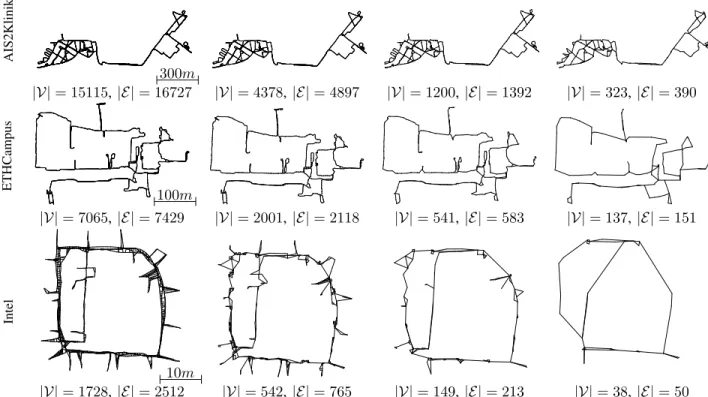
AIS2Klinik
300m
|V|= 15115,|E|= 16727 |V|= 4378,|E|= 4897 |V|= 1200,|E|= 1392 |V|= 323,|E|= 390
ETHCampus
100m
|V|= 7065,|E|= 7429 |V|= 2001,|E|= 2118 |V|= 541,|E|= 583 |V|= 137,|E|= 151
Intel
10m
|V|= 1728,|E|= 2512 |V|= 542,|E|= 765 |V|= 149,|E|= 213 |V|= 38,|E|= 50
Fig. 2. Hierarchies computed by SMF for different datasets. The picture shows the separator graph at different levels, with the number of nodes and edges.
partition induces a partitioning on the edge set into two subsets:
ES andEM, with EM =EM
1 ∪ · · · ∪ EmM andES∪ EM =E. The setEM
i contains edges which connect only the nodes in
VI
i andES is the edge-cut set that connects nodes from two different subgraphs. EachVI
i is then subdivided in the set of boundary nodes VS
i and a set of interior nodes V M i , where VI i =V M i ∪ V S i ,V S
i are those nodes ofV I
i which are incident with at least one edge fromES, andVM
i ∩ V S i =∅. Let xM n = S j∈VM n xj and x S n = S j∈VS nxj. We can
decompose the distributionp(z|x)in Eq. (1) according to: p(x|z) = p(xM,xS |z) Bayes = p(xM |xS,z)p(xS |z) M arkov = m Y n=1 p(xMn |xSn,zMn )p(xS|z), (2) where xM = S nx M n , xS = S nx S n, zMn = {zij | {i, j} ∈ EM
n } and the rightmost part stems from the global Markov property.
Equation Eq. (2) defines the building blocks of our hierarchy. The bottom level of the hierarchy consists of the mdisjoint subgraphs GM
n induced from the distributionsp(xMn |xSn,zMn ). The top level is the graph of the separatorsGS and is induced by the distribution p(xS |z). Figure 1 shows an example of a two-level hierarchy. Multiple levels are then iteratively built, considering the previously computed separator graph GS as the input graph G and performing the decomposition on it.
To design a low-memory-consumption algorithm, we require that the size of all the partitions on every level is small enough to fit into memory. In principle, one can use every
partitioning algorithm with this property. Potential candidates are METIS [13] or Nibble [22]. In our current implementation we have opted for Nibble because it is a local algorithm and it is able to generate graph partitions in an incremental fashion. Accordingly it does not require to store the whole graph in memory.
B. Leaves-to-Root Coarsening
The purpose of the leaves-to-root inference is to compute, at each level of the hierarchy, the marginal distributionp(xS |z) of the separator graphGS. Exploiting the pairwise nature of the SLAM graphical model, as been done for Eq. (1), we have
p(xS |z) = Z p(xM,xS|z)dxM ∝ Y zij∈zS φzij(xi,xj) m Y n=1 Z Y zuv∈zMn φzuv(xu,xv)dxMn . (3)
This decomposition tells us that the marginal distribution of the separator nodes is composed of the factors coming from the separator edges, connecting the boundary nodes of two different partitions, and the factors computed by marginalizing out the inner nodes of each partition, connecting the boundary nodes of the same partitions. The process of marginalization may destroy the original sparseness of the pose-graph, leading to high computational costs and memory requirements. To avoid this, we propose to approximate the full marginal distribution of the boundary nodes with a tree-structured distribution that preserves the marginal mean.
Chow and Liu [2] showed that the tree-structured distribution that minimizes the Kullback-Leibler divergence can be obtained
Fig. 3. Example construction of the approximate separator graph for a single partition. The left image shows the original graph, where the separators are displayed as squares and thicker lines depict the maximum spanning tree. The right image shows the resulting separator graph obtained by performing the depth-first visit.
by computing the maximum spanning tree on the mutual information graph. Although their proof considers discrete distributions, the result holds also for continuous densities. Unfortunately, computing the mutual information between boundary nodes involves inverting the information matrix relative to the entire subgraph, resulting in a computationally expensive operation.
We instead build a maximum spanning tree of the measure-ment information, where the graph structure is the same as
GM
n and the edges are weighted according to det(Ωij). We build the approximate separator graph incrementally. First, we optimize the partition without considering the separator edges. Second, we compute the maximum spanning tree T with one of the separators as root node and the path Pij on the tree connecting the nodesiandj. By performing a depth-first visit on the tree, we select the edges of the graph such that any separator is connected to its closest parent in T, resulting in the edge set ET. For each edge (i, j) ∈ ET, we compute a
virtual measurement z∗ij = M k∈Pij ˆ zk,k+1 (4) Ω∗−ij 1=JΩ−P1ijJ T, (5)
where J is the Jacobian of Eq. (4), ˆzk,k+1 = ˆxk xˆk+1 is
the transformation between node k and k+ 1 in the path, after optimization, and ΩPij is a block diagonal matrix,
whose diagonal elements correspond to the information matrix associated to the edges on the path. In practice, we compute the covariance matrix Ω∗−ij 1 by propagating the covariance matrices of the measurements along the compounding path [21]. Figure 3 shows an example construction of the separator graph for a single partition. We iterate this process of fine-to-coarse optimization until we reach the top level of the hierarchy. Note that any nonlinear least-squares optimizer can be used for the optimization of the subgraphs, in our current implementation we use g2o [15] for that purpose.
C. Root-to-Leaves Optimization
Once the hierarchy has been built, we obtain a solution for the top-most separator nodes by solving the corresponding least square problem. To obtain the final map, we need to propagate the solution obtained to the leaves of the hierarchy. In case of linear systems, this propagation is equivalent to back
Fig. 4. One example Manhattan world dataset used in the memory consumption experiment.
substitution. To overcome the non-linearities of SLAM, we propose to perform an additional optimization step on each subgraph, by fixing the separator variables and only minimizing with respect to the inner nodes. This step corresponds to N independent minimization problems of limited size, one for each subgraphGM
n . The process is then iterated for each level in the hierarchy.
The least square minimization algorithm is always applied to bounded problems. The partitions are bounded by construction, due to the partitioning algorithm. The separator graph is also bounded by construction. The number of separator nodesS is smaller than the number of original nodes, since the separators are a subset of the nodes of the original graph. The number of edges is also bounded, since we only consider the edges between separators from the original graph and theS−1edges connecting the separator of a single partition.
IV. EXPERIMENTS
We evaluate our approach (SMF) with respect to memory consumption, runtime on low memory systems and metric accuracy and compare it to other state-of-the art mapping approaches, namely TSAM21 [19], GTSAM2 [11], g2o3 [15].
To investigate the properties of our approximation, we com-pare our method to two other non-exact solvers, which are HogMan4 [7] and a variant of TSAM2 that does not perform
subgraph relaxation (T2-NOREL). Throughout the experiments, we limited the maximum submap size to500nodes. We ran all approaches on a single thread and without any parallelization using Ubuntu 12.04 on an i7-2700K processor running at 3.5GHz. Note that HogMan runs incrementally, while all others are batch solvers.
A. Memory Consumption
In the first experiment, we evaluated the memory footprint on large-scale and synthetically generated datasets of Manhattan-like worlds, see Fig. 4. The corresponding maps have graphs whose number of nodes ranges between 20,000 and 500,000 and whose connectivities lead to up to two millions edges. To
1We thank the authors for providing their own implementation 2ver. 2.3.1 – https://collab.cc.gatech.edu/borg/gtsam/
3ver. git455 – https://github.com/RainerKuemmerle/g2o 4ver. svn20 – http://openslam.org/hog-man.html
0.1 0.2 0.5 1.0 2.0 5.0 10.0 0 100 200 300 400 500
Memory [GB] in logarithmic scale
number of nodes [thousands] SMF g2o GTSAM TSAM2 T2-NOREL HogMan
Fig. 5. Memory consumption of modern SLAM solvers compared to our approach on large-scale graphs. Please note that the y-axis has logarithmic scale. 1 5 10 20 30 40 0.5 0.75 1 Time [min] Memory [GB] SMF g2o GTSAM TSAM2 T2-NOREL
Fig. 6. Runtime comparison with memory constraints.
investigate the memory consumption, we employedvalgrind and massifin a native Linux environment. Both are open source tools for process memory analysis.
Figure 5 shows the results of the experiment. The graph shows two important aspects. First, our approach has the lowest memory consumption: it is constantly almost one order of magnitude more memory efficient than TSAM2, up to 2 times more than g2o and GTSAM, and up to 1.3 times more than T2-NOREL and HogMan. Even though SMF, HogMan and T2-NOREL have a similar memory footprint, SMF is substantially more accurate, as shown in Section IV-C. Second, the approximate methods HogMan, SMF, and T2-NOREL) have lower memory consumption than the exact methods TSAM2, g2o, and GTSAM.
B. Runtime on Systems with Restricted Main Memory
This experiment evaluates the computation time on systems with restricted main memory. For simulating these systems, we limited the available memory for the Linux kernel. We evaluated three budgeted memory settings (0.5GB, 0.75GB and 1.0GB) on 15 synthetic datasets with 200,000 nodes and varying connectivity. The mean number of edges was 640,000 with a standard deviation of 78,800.
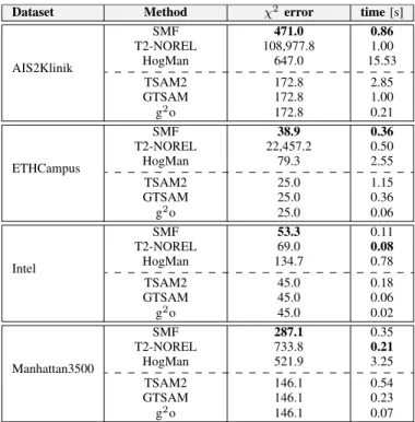
TABLE I
SMALLMEMORYFOOTPRINTMAPPING(χ2, TIME)
Dataset Method χ2 error time[s]
AIS2Klinik SMF 471.0 0.86 T2-NOREL 108,977.8 1.00 HogMan 647.0 15.53 TSAM2 172.8 2.85 GTSAM 172.8 1.00 g2o 172.8 0.21 ETHCampus SMF 38.9 0.36 T2-NOREL 22,457.2 0.50 HogMan 79.3 2.55 TSAM2 25.0 1.15 GTSAM 25.0 0.36 g2o 25.0 0.06 Intel SMF 53.3 0.11 T2-NOREL 69.0 0.08 HogMan 134.7 0.78 TSAM2 45.0 0.18 GTSAM 45.0 0.06 g2o 45.0 0.02 Manhattan3500 SMF 287.1 0.35 T2-NOREL 733.8 0.21 HogMan 521.9 3.25 TSAM2 146.1 0.54 GTSAM 146.1 0.23 g2o 146.1 0.07
Figure 6 shows the average runtime of all the batch solvers (g2o, GTSAM, TSAM2, T2-NOREL and SMF). SMF is the
fastest method at the lowest memory setting and comparable to T2-NOREL at increasing memory setups. All the other methods are significantly slower. In the lowest memory setup, TSAM2 was frequently killed by the kernel and was successful only 3 out of 15 trials. In the same setting, GTSAM never terminated.
To evaluate the statistical significance of the results, we performed a paired sample t-test with a significance level α= 0.05. The test shows that SMF is2 times faster than g2o on 0.5GB, 1.6 times on 0.75GB, and1.7times on 1GB. With respect to TSAM2, SMF is8times faster on 0.75GB and10 times faster on 1GB, where on 0.5GB no significant result can be given due to the limited amount of successful trials. SMF is also7.2times faster than GTSAM on 0.75GB and3.7 times faster on 1GB. The timing performance of T2-NOREL is very similar to SMF, with SMF being1.4times faster on 0.5GB settings. Note, however, that SMF is substantially more accurate than T2-NOREL as shown in the next section.
C. Metric Accuracy
In these experiments, we quantified the metric precision of all the SLAM solvers and the time required to provide a solution without constraining the amount of available memory. Here, we run the solvers on several publicly available datasets: AIS2Klinik (15,115 nodes, 16,727 edges), ETHCampus (7,065 nodes, 7,429 edges), Intel (1,728 nodes, 2,512 edges) and Manhattan3500 (3,500 nodes, 5,542 edges). These datasets have been selected because they are good representatives of different environments (indoor and outdoor), simulated and real-data.
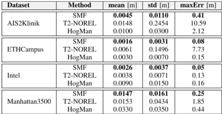
TABLE II
SMALLMEMORYFOOTPRINTMAPPING(RPE)
Dataset Method mean[m] std[m] maxErr[m]
AIS2Klinik SMF 0.0045 0.0110 0.41 T2-NOREL 0.0148 0.2454 10.59 HogMan 0.0100 0.0300 2.12 ETHCampus SMF 0.0016 0.0031 0.08 T2-NOREL 0.0061 0.1496 7.73 HogMan 0.0030 0.0070 0.15 Intel SMF 0.0026 0.0037 0.05 T2-NOREL 0.0038 0.0071 0.13 HogMan 0.0090 0.0150 0.16 Manhattan3500 SMF 0.0147 0.0161 0.25 T2-NOREL 0.0153 0.0434 1.85 HogMan 0.0330 0.0350 0.44
Tab. I summarizes the results with respect to theχ2 error
and runtime. Bold numbers indicate the best result among the approximate methods. Out of the approximate solvers, SMF has the lowest error and the lowest runtime in all the datasets but Intel and Manhattan3500, where T2-NOREL is slightly faster. SMF is more accurate than T2-NOREL: from500times on the ETHCampus dataset to 1.3 times on the Intel one. Compared to HogMan, SMF is up to 2times more accurate and up to10 time faster. With respect to the exact solvers, SMF achieves comparable accuracy in all the datasets, being slightly slower than GTSAM and g2o and slightly faster than TSAM2.
In order to precisely assess the quality of map reconstruction, we have also computed the reprojection error (RPE) between every edge of the optimized graph and the ground truth map computed using an exact solver – g2o in our case.
Tab. II summarizes the results of the evaluation, showing the RPE mean, standard deviation and maximum error. SMF is more accurate than T2-NOREL and HogMan in all datasets. This is particularly evident on the two large outdoor datasets AIS2Klinik and ETHCampus where SMF is 3 times more accurate than T2-NOREL with respect to the mean error and more than an order of magnitude with respect to the maximum error. SMF is also up to 3 times more accurate than HogMan for the mean error and up to 4 times with respect to the maximum error. From a robot navigation standpoint, maximum-errors are indicators of how far some parts of the map are misaligned. Large values of this error may render the map unusable because, e.g., paths could not be computed: this happens with T2-NOREL in datasets AIS2Klinik (≥10m) and ETHCampus (≥7m). In those datasets, SMF instead achieves maximum-error of 0.4mand0.08m.
V. CONCLUSIONS
In the past, solutions for solving the SLAM problem mostly focused on accuracy and computation time. In this paper, we also considered memory constrained systems and presented a novel hierarchical and approximated SLAM technique that produces accurate solutions thereby requiring only a small memory footprint. Our solution is particularly appealing for solving large-scale SLAM problems or for setups with limited memory. Our experimental results suggest that our approach
uses significantly less memory than state-of-the-art systems and is significantly faster on systems with restricted main memory. At the same time, it yields an accuracy that is comparable to that of state-of-the-art solvers.
REFERENCES
[1] M. Bosse, P. Newman, J. Leonard, and S. Teller. An ATLAS framework for scalable mapping. InIEEE Int. Conf. on Rob. & Aut. (ICRA), 2003. [2] C. Chow and C. Liu. Approximating discrete probability distributions
with dependence trees.IEEE Tran. on Inf. Theory, 14(3), 1968. [3] C. Estrada, J. Neira, and J. Tard´os. Hierachical SLAM: Real-time accurate
mapping of large environments.IEEE Trans. on Rob., 21(4), 2005. [4] U. Frese, P. Larsson, and T. Duckett. A multilevel relaxation algorithm
for simultaneous localisation and mapping. IEEE Tran. on Rob., 21(2), 2005.
[5] U. Frese. Treemap: An O(log n) algorithm for indoor simultaneous localization and mapping. Aut. Rob., 21(2), 2006.
[6] G. Grisetti, C. Stachniss, and W. Burgard. Non-linear constraint network optimization for efficient map learning. IEEE Tran. on Intel. Transp. Sys., 10(3), 2009.
[7] G. Grisetti, R. K¨ummerle, C. Stachniss, U. Frese, and C. Hertzberg. Hierarchical optimization on manifolds for online 2D and 3D mapping. InIEEE Int. Conf. on Rob. & Aut. (ICRA), 2010.
[8] G. Grisetti, R. K¨ummerle, and K. Ni. Robust optimization of factor graphs by using condensed measurements. InIEEE/RSJ Int. Conf. on Intel. Rob. and Sys. (IROS), 2012.
[9] J.-S. Gutmann and K. Konolige. Incremental mapping of large cyclic environments. InIEEE Int. Symp. on Comp. Intell. in Rob. and Aut., 1999.
[10] A. Howard, M. Matari´c, and G. Sukhatme. Relaxation on a mesh: a formalism for generalized localization. InIEEE/RSJ Int. Conf. on Intel. Rob. and Sys. (IROS), 2001.
[11] M. Kaess, H. Johannsson, R. Roberts, V. Ila, J. Leonard, and F. Dellaert. iSAM2: Incremental smoothing and mapping using the Bayes tree.
Int. Jour. of Rob. Res., 31, 2012.
[12] M. Kaess, A. Ranganathan, and F. Dellaert. iSAM: Fast incremental smoothing and mapping with efficient data association. In IEEE Int. Conf. on Rob. & Aut. (ICRA), 2007.
[13] G. Karypis and V. Kumar. Multilevel k-way partitioning scheme for irregular graphs. Jour. of Par. and Distr. Comp., 48, 1998.
[14] H. Kretzschmar and C. Stachniss. Information-theoretic compression of pose graphs for laser-based slam.Int. Jour. of Rob. Res., 31, 2012. [15] R. K¨ummerle, G. Grisetti, H. Strasdat, K. Konolige, and W. Burgard.
g2o: A general framework for graph optimization. InIEEE Int. Conf. on Rob. & Aut. (ICRA), 2011.
[16] R. K¨ummerle, M. Ruhnke, B. Steder, C. Stachniss, and W. Burgard. A navigation system for robots operating in crowded urban environments. InIEEE Int. Conf. on Rob. & Aut. (ICRA), 2013.
[17] F. Lu and E. Milios. Globally consistent range scan alignment for environment mapping. Aut. Rob., 4(4), 1997.
[18] K. Ni, D. Steedly, and F. Dellaert. Tectonic SAM: exact, out-of-core, submap-based slam. InIEEE Int. Conf. on Rob. & Aut. (ICRA), 2007. [19] K. Ni and F. Dellaert. Multi-level submap based slam using nested
dissection. InIEEE/RSJ Int. Conf. on Intel. Rob. and Sys. (IROS), 2010. [20] E. Olson, E. Leonard, and S. Teller. Fast iterative optimization of pose graphs with poor initial estimates. InIEEE Int. Conf. on Rob. & Aut. (ICRA), 2006.
[21] R. Smith, M. Self, and P. Cheeseman. Estimating uncertain spatial realtionships in robotics. InAut. Rob. Vehicles. 1990.
[22] D. A. Spielman and S.-H. Teng. Nearly-linear time algorithms for graph partitioning, graph sparsification, and solving linear systems. InACM Symp. on Th. of Comp., 2004.
[23] H. Strasdat, A. J. Davison, J. M. M. Montiel, and K. Konolige. Double window optimisation for constant time visual slam. InInt. Conf. on Com. Vis. (ICCV), 2011.
[24] S. Thrun, M. Montemerlo, H. Dahlkamp, D. Stavens, A. Aron, J. Diebel, P. Fong, J. Gale, M. Halpenny, G. Hoffmann, et al. Stanley: The robot that won the darpa grand challenge.Jour. of Field Robotics, 23(9), 2006. [25] C. Urmson, J. Anhalt, D. Bagnell, C. Baker, R. Bittner, M. Clark, J. Dolan, D. Duggins, T. Galatali, C. Geyer, et al. Autonomous driving in urban environments: Boss and the urban challenge.Jour. of Field Robotics, 25 (8), 2008.