Economic Growth and Public Debt
Keshab Bhattarai
University of Hull, Business School
April 1, 2016
Abstract
There is a controversy in the literature about the economic contribution of public de…cit. Keynesian economists generally argue that by spending more on goods and services and in-frastructure possible budget de…cit is helpful to create more jobs, reduce unemployment rate and raise the rate of economic growth of an economy. Neoclassical economists are worried about the adverse consequences of public de…cit on capital accumulation and economic growth rate. Under classical Ricardian equivalence proposition private savings o¤sets public dis-saving thus budget de…cit does not matter in the long run. Development economist often warn against the adverse consequences of budget de…cit on in‡ation, current account balances and redistri-bution of income. Empirical evidence is found for a positive or a negative or no e¤ect of debt on growth. Debt promote growth if it is used for investment and harms growth if it is used for consumption. Whether debt is more for investment or consumption depends on economic and political circumstances of a country.
Key words: Growth, in‡ation, budget de…cit JEL Classi…cation: C68, D63, O15
This paper was presented at the European Economics and Finance Conference in Brussels in June 2015. Address: Cottingham Road, Hull, HU6 7RX. Phone: 441482463207; Fax: 441482463484; email: K.R.Bhattarai@hull.ac.uk
1
Introduction
The major objectives of …scal policy in any country include 1) macroeconomic stabilisation for higher growth rate of output, full employment, stable prices, interest and exchange rates and low in‡ation 2) attaining horizontal and vertical equity through taxes and transfers and achieving e¢ ciency in resource allocation and provision of public goods; 3) maximizing positive externality by investing in public services such as health and education and minimising the negative externality through appropriate taxes and subsidies. Direct taxes on income, pro…t and wealth and indirect taxes including VAT, tari¤, excise, business and subsidies on goods and services and for use of inputs and spending on pure public goods (defence, law-order, national parks and semi-public goods) including education, health and R&D are major instruments to achieve these objectives. When the revenue from taxes, the compulsory payments from citizens to the government, in return of public services are not enough to meet public spending government borrows from the private sector. It crowds out private investment raising interest rate, in‡ation as well as the current account de…cit while it borrows from the central banks.
There is a controversy in the literature about the economic contribution of public de…cit. Key-nesian economists generally argue that by spending more on goods and services and infrastructure, budget de…cit is helpful in creating more jobs, reducing the unemployment rate and raising the eco-nomic growth rate of the economy. Neoclassical economists are more concerned about the adverse consequences of public de…cit on capital accumulation and economic growth. Classical economists under Ricardian equivalence proposition argue that private saving and public de…cit (dis-saving) o¤set each other. Despite this all recognise the adverse consequences of excessive budget de…cit on in‡ation, current account balances and redistribution of income. How much budget de…cit in‡uences real choices of people through its impact on economic growth is essentially an empiri-cal issue. Enough debates have taken place regarding the optimal size of the government (Pigou (1947), Samuelson (1954), Buchanan (1965), Atksinson and Stern (1974), Feldstein (1974), Whal-ley (1975), Boadway (1979), Summer (1980), Blomquest (1985), Bovenberg (1989), Benabou (2002) and Taveres (2004)).
Whether de…cit is good, bad or insigni…cant partly depends on which of these paradigms one tends to believe. Barro (1974, 1989) argues for the Ricardian equivalence theory - households with perfect foresight maintain balance between the present value of their income and expenditure and internalise the public de…cit through intertemporal optimisation raising savings to make up for anticipated higher tax rates in the future. This result may not apply when households face lending and borrowing constraints. Aiyagari et al. (2002) use a stochastic Ramsey model to prove that intertemporal balance is essential for maximising welfare but budget need not to be balanced on a continual basis. They favour tax and expenditure smoothing policies when both of these are subject to random shocks. Burnheim (1989) denounces Ricardian view in favour of New-Keynesian
propositions. He draws parallels between these two and suggests decomposing de…cit into permanent and temporary parts. In the neoclassical model where farsighted individuals plan consumption over lifetime, budget de…cit raises lifetime consumption by shifting taxes to the next generation; this raises consumption and lowers savings and raises interest rate. Public sector de…cit then crowds out private investment. As Diamond (1965) and Auerbach and Kotliko¤ (1986) demonstrated high debt to GDP ratio depresses capital labour ratio. Ni and Wang (1995) have proven how high saving …scal policy regime with lower public sector de…cit enhances long run growth rate of the economy. In contrast Keynesian models show positive multiplier e¤ect of budget de…cit on income and consumption- which is just inverse of the marginal propensity to save. Beetsma and Giuliodori (2011) using VAR impulse response analysis have found positive impacts of government purchases among EU countries. Based on major theoretical paradigms this paper aims to provide empirical evidence to support in favour or against these theories and reexamine the claim that there is a weak link between de…cit and income.
2
Theories on public debt
2.1
Ricardian Equivalence and Neoclassical Arguments on Debt
Ricardian equivalence means that individual households save more in response to a rise in the budget de…cit now so that they will be able to pay higher rates of taxes when the government imposes on them when repaying those debts in the future. The household budget constraint shows how the accumulation of public debt(Bt+1)and private asset(At+1)in t+ 1period relate to the current income from wages(WtNt), pro…ts( t), interest income on bonds(1 +Rt)Bt and income
on assets(1 +RAt)Atand expenses on consumption(Ct)and taxes(Tt).
Bt+1+At+1=WtNt+ t Tt Ct+ (1 +Rt)Bt+ (1 +RAt)At (1)
Changes in government borrowing occurs due to di¤erence in government spending and taxes and the interest rate payment on outstanding debt. Thus the government’s budget constraint becomes:
Bt+1 Bt=Gt Tt+RtBt=)(1 +Rt)Bt=Bt+1 Gt+Tt (2)
Putting government budget into the household budget constraint
Bt+1+At+1=WtNt+ t Tt Ct+Bt+1 Gt+Tt+ (1 +RAt)At (3)
At+1=WtNt+ t Ct Gt+ (1 +RAt)At (4)
Thus in the classical spirit the larger public sector (Gt) implies smaller private sector assets
(At+1). Then the dynamic equilibrium with this constraint implies market clearing in each period.
Yt=WtNt+ t=Ct+Gt (5)
2.2
Role of Debt in a Keynesian Model
Marginal propensity to consume with lump-sum or proportional taxes are key components in a Keynesian model of government spending.
Y =C+I+G (6)
C=a+b(Y T); a >0,0< b <1 (7)
Assume that tax(T) is collected lump sum and de…cit (G T) is …nanced by borrowing (B) when tax(T)is not enough to meet expenses (G).
G=T+B (8)
Rearrange for a matrix:
Y C=I+T +B (9) bY +C=a bT (10) Y C ! = " 1 1 b 1 # 1 I+T+B a bT ! (11) Using Cramer’s rule
Y = (I+T+B) + (a bT)
1 b (12)
C= (a bT) + (I+T+B)
Y =a+I+ (1 b)T
1 b +
B
1 b (14)
Thus the budget de…cit will have direct impact on output and consumption by the Keynesian multiplier, @Y@B = 11b >0 or @C@B =11b >0: In this set up @Y@T = 1 and @C@T = 1 a balanced budget multiplier e¤ect is achieved when budget is exactly balanced, B= 0. By log di¤erentiation it can be shown that growth rate of GDP depends on the percentage change in the public borrowing:
gY = 1+ 2gB (15)
Here 1 can be negative or positive or zero ( 1 7 0) depending how the positive e¤ect of investment compares to the negative impact of taxes. Normally it should be 1>0. The Keynesian model implies 2>0:
This model can be extended to an open economy model by adding exports and imports in the aggregate demand functions. It can include in‡ation making the interest rate subject to the real interest rate and using the Fisher equation. With these modi…cations the model becomes:
Y =C+I(r) +G+X IM (16)
r= i (17)
IM =mY (18)
Y =C+I( i) +T+B+CA (19)
X IM =Y C I(r) G=Y C I(r) T B (20)
If the investment and savings in the private sector are balanced this simply becomes:
X IM = (T+B) (21)
Whilst a central bank determines the nominal interest rate the in‡ation is determined from the money market where the demand for money required for transactions or precautionary purposes equals the supply of money, which itself is in…nitely elastic given the central bank’s commitment to a certain interest rate.
M
P =kL( i) +f Y (22)
Taking log di¤erentiation of this function in‡ation is the di¤erence between the growth rate of money supply and the sum of growth rate of output and liquidity as:
=gm gy gL (23)
From this equation one could link in‡ation, current account de…cit and de…cit to the growth rate of the economy.
gY = 1+ 2gB+ 2 + 2gCA+e (24)
From this equation one could argue that higher government de…cit will lead to higher growth but this e¤ect could be o¤set by in‡ation and the current account de…cit. For a sustainable debt in‡ationtax component of bet should be = P YM =G TY + (i g)BY:1
2.3
New-Keynesian business cycle model
Neo-Keynesian business cycle model with leisure and consumption in the utility functions and a stochastic technology of production is expressed in the following form:
max E "1 X t=0 tU(C t+i; Lt+i)j t # (28) subject to: Nt+i+Lt+i= 1 (29) Ct+i+St+i=Zt+iF(Kt+i; Nt+i) Gt+i (30) Kt+i 1= (1 )Kt+i+St+i (31)
First order conditions imply that the disutility from labour should equal the marginal utility
1 (P B) P Y + M P Y = P G P T P Y +i P B P Y (25) P B P Y + B Y = G T Y +i B Y M P Y (26) B Y = G T Y + (i g) B Y M P Y (27)
from work as:
V0(Lt+i) =
Wt
Ct
(32) The …rst order condition for optimisation:
E (1 +rt+1) Cit Cit+1 j t = 1 =E Rt+1 Ct Ct+1 j t (33) The New Keynesian model thus suggests that the higher government spending leads to lower private consumption but the decrease is less than one to one. It raises output and employment. Taxes go up if increase inGtis permanent and investment is lower. Higher the transitory component
ofGtlower will be its in‡uence in output. Substitution and income e¤ects work; taxes are highly
discretionary and distortionary. Optimal size of public sector, thus, is a political issue. Higher the transitory component of output, smaller the decrease in consumption and greater the impact on output. Ricardian equivalence fails.
2.4
Impacts of public de…cit in the Neoclassical growth model
Impacts of public de…cit in a neoclassical growth model could be based on studies of Feldstein (1974), Whalley (1975), Boadway (1979), Summer (1980), Blomquest (1985), Bovenberg (1989), Rankin (1992), Ni and Wang (1995), Benabou (2002). Larger public sector de…cit is found to be harmful for long term growth in neoclassical growth models where households choose the optimal path of consumption and accumulation of capitalfct; ktg1t=1in response to public policy that includes plan of taxes and public expendituref ; gg1t=1. Particularly the household’s optimisation problem is:
max 1 X t=0 tU(c t) (34) subject to ct+kt+1= (1 t)f(kt) t 0 (35)
Euler equation implied by this equals:
Uc((1 t)f(kt) kt+1) = Et(1 t+1)Uc((1 t+1)f(kt+1) kt+2)f0(kt+1) (36) When government is forced to operate a balanced budget every period the link between tax revenue and public spending is given by:
tf(kt) =G (37)
When government is allowed to operate a structural balance it is permitted to intertemporally balance the budget
f(kt) +
bt+1 1 +rt
=b+G (38)
Balancing the budget in the entire model horizon would imply
f(k0) G+ 1 X t=1 8 > < > : tf(kt) G t 1 t=0(1 +rt) 9 > = > ;= 0 (39) Uc((1 t)f(kt) kt+1 G) = Et(1 t+1)Uc((1 t+1)f(kt+1) kt+2 G)f0(kt+1) (40) In steady sate (1 )f0(k) = 1 (41) 1 G f0(k) f0(k) = 1 (42) G(k) = 1 G f0(k) f0(k) = 1 (43) Positive e¤ect of public sector …nances is possible only when ratio of public spending to the marginal productivity of capital (tax rate) is less than one, 1 f0G(k) >0:
2.5
Cause of a debt crisis
LetRbe the risk free payo¤ for investors andR be the return on government bonds. Let be the probability of default. Then an arbitrage condition implies
(1 )R=R (44)
Some arrangement yields:
= R R
As the probability of default rises the government need to pay higher interest rate, as shown by line D in the graph.
Then the government retire debt if T =RD . This implies T
D =R. When the interest rate is
low, as at point A, the collected tax revenue is likely to be enough to serve the debt and therefore probability of default( )on public debt is zero. Then 0 < <1 between A and B points and probability of default line is shown by line T. After point T the probability of default is 1 therefore the government cannot borrow even paying very high interest rate and R =) 1.
When more than one period is involved, then beliefs of other people about the possibility of default in the next period a¤ects the decision whether to purchase a bond at the current period. Beliefs about beliefs about beliefs and thus leads to a self ful…lling crisis.
One could apply above model in the context of current debt crises faced by Greece, Spain or Portugal in recent years. This is one of the reason why the UK government would like to limit debt GDP ratio at the reasonable rate of around 76 percent (See Romer (2006), Calvo (1988), Cole and Keheo (2000)).
3
Credibility:Dynamic Programming Squared (DPS)
Ljungqvist and Sargent (2012) characterise the values of a government that are consistent to sus-tainable reputation using dynamic programming squared (dps) concept following Abreu Pease and Stachetti (1986, 1990) to deal with a set of value functions associated to the history of a set of strategy pro…les of households and governments. On one side they show equivalence of the debt pro…les in the rational expectation to that in the competitive equilibrium and they compare these to the debt pro…les in the Nash equilibrium. Reputation is subject to ability to commit. This
requires forming a strategy space that is history dependent. Reputation could be based on the rational expectation. Credibility is based on beliefs and it leads to the theory of government. They will do as this is in their interest and feasible. Motives of the government is included along with that of the households in a dps model.
Household h chooses consumption 2 X and the private sector average x2 X. The public sector choosesy, e.g. in‡ation. Utility isu( ; x; y); when x=Q y= t+j. This generates
choice problem:
max
2X u( ; x; y)
where choice of household depends on average choice(x)and public policy(y): =f(x; y). The rational expectation equilibrium is equivalent to competitive equilibrium:REE sCE; x=f(x; y)
Set of competitive equilibrium
C=) f(x; y) ; X=h(g)g
For instance in a Ramsey problem, the government choosesy knowingx= ln (y)
max
y2Y u(h(y); h(y); y) = max(x;y)2C u(x; x; y) =)V R; yR
While the solutions of the Nash equilibrium XN; yN satis…es the competitive equilibrium
XN; yN 2 C, but the Nash solutions are inferior to the rational expectation solutions,G, XN,
u XN; Xv; yG = max
2Y u(x
0; x0; ) =)VN; yN andVN < VR:
Reputational choice is history dependent. An example of Ljungqvist and Sargent (2012) chapter 22: u(l; c; g) =l+ lg ( +c) + lg ( +g) ; 2 0;1 2 l+g= 1 +l ; ( ; g)sy l( ) =f1 if 2(0;1 ) 1 if >1 History t2X 8t;xt2X 8t; yt2X 8t fort11 Vg !x ;!y = 1 X1 t=0 t r(xt; yt) ; 2(0;1) ! x ;!y =f(xt; yt)g1t=0
Reputation means choice attis a function oft 1
yt= Xt 1; Yt 1
3.1
Dynamic programming square
LetV be the value to government in the …rst period of following the policy that the private sector had expected.
LetV1be the continuation value of known policy.
LetV2 be the continuation value if the private sector believes that the government choice is not what they expect.
V = (1 )u(x; x; y) + V1 > (x;y)2C
(1 )u(x; x; ) + V2 ; 8 2Y A strategy pro…le implies a trajectory of outcome (x; y)and a value function
Vg( ) =Vg[x( ); y( )]
and continuation pro…le j(x;y); j(x ;y ):
A strategy pro…le is a sub-game perfect equilibrium (SPE) of in…nitely repeated economy if 8
t>1and 8(xt; yt)2 Xt 1; Yt 1
a)xt= ht Xt 1; Yt 1 is consistent with the competitive equilibrium where g t Xt 1; Yt 1 b)8 2Y (1 ) (xt; yt) + Vg j(x;y) > (x;y)2C (1 ) (xt; ) + Vg j(x; )
According to Sargent "there should be people in the model to be realistic" and "…nding the state is an art" Similarly for Lucas "complete markets are all alike but each incomplete markets are incomplete in their own way". The 0dynamic problems of debt due to incomplete markets strategic interactions among households and forms requires evaluating multiple states of budgets, information reputation and commitment. For instance consider a simple economy with villagers and a money lender. Villager’s objective is to maximise the expected utilityEP1
t=0
tU(C
t); (0,1);
U0(:)>0andU00(:)<0Ctii =1...N.yitshould be a random process given by the joint density. This
endowment economyyi
t iidprob yit=y=ys : Complete market case is the AD style contingent
commodity market and leads to complete consumption smoothing. ci t = c =
1
P
t=0
ys s: across all
individual and states. Good is not storable; three possible cases arise a) villager cannot commit but
money lender can borrow and c) villager can commit and save and borrowyi
t not observed. This
brings to the theory of distribution among the villages and money lenders and strategies for the government either a) chooses sequence of t+j once and walks away and b) choosing sequence of
t+j in each period. This requires ideas of game in the modelling as above.
4
Empirical Analysis
Economic and political beliefs and circumstances keep changing in response to new opportunities and di¢ culties which augment theoretical controversy regarding the relationship between growth and public debt. As the public decisions a¤ect millions of households and …rms and their reactions to announced or anticipated policies vary the empirical analysis of the link becomes of great public interest. Here data on growth, de…cit, current account and several macroeconomic variables are obtained for advanced countries from the World Economic Outlook database of the IMF from 2000 to 2010 including the IMF forecasts for up to 2015.2 This data set is used here to examine whether the public de…cit helpful or harmful for economic growth and whether de…cit stabilises or destabilises an economy in terms of its impact on in‡ation and current account de…cit. Regression coe¢ cients of de…cit or a set of variables including de…cit multiple explanatory variables are estimated using the OLS or GLS models and examining their validity on the basis oft; F, 2 andR2 tests. These empirical …ndings imply that:
1. Public borrowing enhances economics growth; borrowing must …nance projects with positive externalities for this.
2. The relationship between the general level of prices and net public borrowing is negative when net borrowing enhances growth and positive when such borrowing funds public consumption. 3. More net borrowing deteriorates the current account balance. As economy grows imports
may increase faster than exports.
Net borrowing a¤ects growth rates and prices di¤erently in di¤erent countries. Time series data from the World Economic Outlook of the IMF is used here to study relationships between growth rates of output and debt ratios among various groups of countries in the world.
4.1
Summary Growth Debt Ratio Regressions
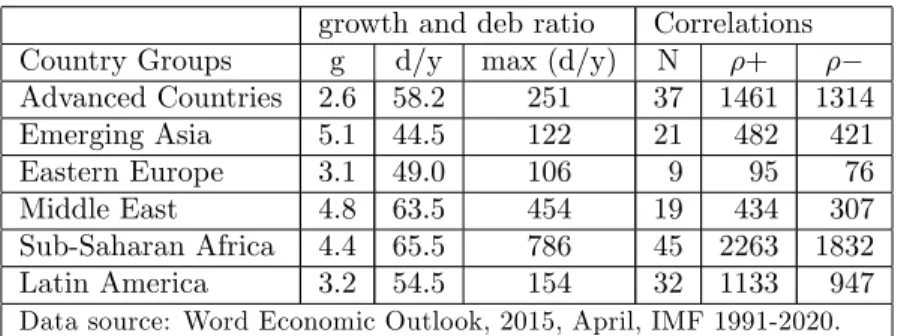
The average growth rates vary signi…cantly across groups of countries; emerging Asia grew on average by 5.1 percent but advanced economies grew by 2.6 on average. The average debt GDP ratio was lowest at 44.5 in Asia and very high at 65.5 in Africa. Maximum debt GDP ratio was
recorded for Africa. Correlations between growth and debt by groups of countries are shown in the last two column. Positive correlations were more frequent than the negative correlations. Causality of debt ratio growth rate are then tested in a set of regressions for each of these countries as shown in Tables 8 to 13.
Table 1: Avege growth rate and debt ratio and the nature of growth deb ratio correltions (1991-2020)
growth and deb ratio Correlations
Country Groups g d/y max (d/y) N +
Advanced Countries 2.6 58.2 251 37 1461 1314 Emerging Asia 5.1 44.5 122 21 482 421 Eastern Europe 3.1 49.0 106 9 95 76 Middle East 4.8 63.5 454 19 434 307 Sub-Saharan Africa 4.4 65.5 786 45 2263 1832 Latin America 3.2 54.5 154 32 1133 947
Data source: Word Economic Outlook, 2015, April, IMF 1991-2020.
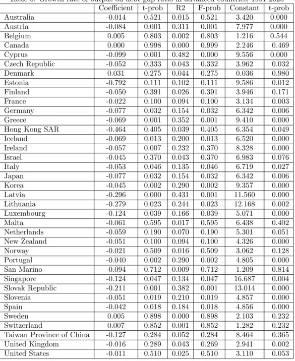
Among advanced countries Hong Kong had the lowest debt ratio at most of 7 percent. Japan had it around 251 percents. Singapore, Korea, Latvia, Lithuania and Estonia grew impressively during this period while the UK and the USA grew by 4 and 4.7 percents respectively. Regression by countries provides evidence for both positive and negative coe¢ cients. Sixteen of these advanced countries had negative and signi…cant impact of deb ratio on growth rates. This relation was insigni…cant in other countries. Thus for advanced countries debt is a¤ecting growth negatively.
Emerging Asian includes large countries such as China, India and Indonesia but also tiny small countries including Bhutan, Maldives Papua New Guinea. While the average debt ratio in Bhutan was up to 122 percent of GDP it was only 3 percent in Borneo. In contrast to regions average rate of 5.1, China was growing at 9.4 and India at 6.7 percent during the study period. Debt ratio had signi…cant and negative impact on economic growth in ten out of twenty one countries of this region. Only Bhutan had positive and signi…cant e¤ect of debt ratio on growth. for others coe¢ cient were insigni…cant.
Debt ratio signi…cantly lowered growth rates in 26 out of 45 countries in Sub Sahran Africa. It had positive impact in three countries such as Benin, Cameroon and Namibia. Coe¢ cients were not signi…cant for other countries. There was wide volatility in growth and debt ratios over time among countries in this region. Debt ratio was more volatile than economic growth rate.
Debt ratio had negative impact on growth rates only in …ve out of nineteen countries in the Middle East, these countries were Algeria, Bahrain, Egypt, Pakistan and the UAE. Debt had harmful e¤ect on growth rate in six out of nine countries in the Eastern Europe. Coe¢ cient of debt ratio on growth regression was signi…cant only six out of 32 Latin America and Caribbean Countries.
From these empirical analysis on grow debt ratio regression it is not possible to state de…nitely that higher debt ratio causes lower growth rate. Whilst the negative impact was observed in many more countries than the positive impacts, number of countries with insigni…cant coe¢ cients is quite high. Is debt used for investment or consumption purposes? If it is for investment purpose higher debt does not lower the GDP growth rate though there are chances that it will raise it. If the debt is used for consumption this will have negative impacts on economic growth. Thus the analysis of debt growth relation would not be complete until the investment or consumption uses of debts are analysed explicitly. Such decomposition is beyond the scope of current analysis as getting such information for all countries included in this empirical analysis is very di¢ cult.
4.2
Analysis of the UK economy
These estimates are tested for heteroskedasticity, autocorrelations and any restrictions as appropri-ate.
Regresses growth rate of output(Yi)on net borrowing(Xi)as:
Yi= 1+ 2Xi+ei i= 1:::T
Following the OLS technique to …nd estimators ofb1 andb2.
b= (X0X) 1X0Y (46)
These estimates are subject to standard OLS assumptions on error terms normality ei
N 0; 2 , homoskedaticity, non- autororrelation (E("i"j) = 0) and independence of errors from
the dependent variables,(E("iXi) = 0).
" b1 b2 # == " N PXi P Xi PXi2 # 1" b1 b2 # = " 12 51:92 51:92 413:52 # 1" 21:3 26:23 # = " 3:283 0:349 # (47) Wherek= number of parameters in the regression;N = number of observations
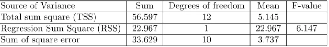
Table 2: Testing overall signi…cance by F-test
Source of Variance Sum Degrees of freedom Mean F-value
Total sum square (TSS) 56.597 12 5.145
Regression Sum Square (RSS) 22.967 1 22.967 6.147
Sum of square error 33.629 10 3.737
Table 3: Growth on net borrowing
Coe¢ cient Standard Error t-value
Intercept 3.283 0.783 4.191
Net borrowing 0.349 0.133 2.613
R2=0.406 ,F = 6:147; N= 12:
Coe¢ cients as well as t-statistics are signi…cant. Autocorrelation is positive becaused= 1:74<2 but that is not statistically signi…cant. The calculated DW value, d = 1:74 is clearly out of the inconclusive region as it does not fall in the range of [0:971;1:331] of the Durbin-Watson table. White test or ARCH and AR test suggest there is slight problem of heteroskedasticity in the errors in this model. However, heteroskedasticity is more serious for cross section than for time series. Therefore conclusion of above model are still valid. One way is to regress predicted square errors
b
e2
i in predicated square of y, Ybi2. The test statistics for normality of errors isnR2 2df with df
=1.
b
e2i = 0+ 1Ybi2+vi ;n:R2= 6:089 (48)
b
e2i = 0+ 1X1;i+ 2X2;i+ 3X12;i+ 4X22;i+ 5X1;iX2;i+vi (49)
Null hypothesis of homoskedasticity is rejected asnR2= 6:089> 2
df = 2:7055.
Table 4: Price index on net borrowing
Coe¢ cient Standard Error t-value
Intercept 102.5 1.603 63.9
Net borrowing -1.85 0.273 -6.76
R2=0.82 ,F = 45:7 [0:00]; N = 12; DW = 1:09
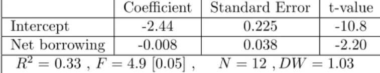
Table 5: Current account balance on net borrowing Coe¢ cient Standard Error t-value
Intercept -2.44 0.225 -10.8
Net borrowing -0.008 0.038 -2.20
R2=0.33 ,F = 4:9 [0:05]; N = 12; DW = 1:03
Prices were relatively stable despite …scal expansion during the study period as the monetary policy mainly concerned in achieving the target in‡ation, had been complementary to the …scal pol-icy in UK in the period of study Table 4. However higher borrowing had caused slight deterioration in the current account, as both consumers and producers tend to import more in response to higher income they received from …scal expansion. There is weak evidence on simultaneity between growth
and de…cit in UK in last ten years. Past records like this may or may not apply for projecting the impacts of current debt reduction plans in the future years; these require analysis of the impacts of such de…cit in the path of economy under dynamic general equilibrium system or under the DSGE or VAR frameworks. One important concept in the literature that handles this issue is the dynamic programming squared presented brie‡y in the next section.
4.3
Conclusion
There is a controversy in the literature about the economic contribution of public de…cit. Keynesian economists generally argue that by spending more on goods and services and infrastructure possible, the public de…cit is helpful to create more jobs, reduce unemployment rate and raise the economic growth rate of the economy. Neoclassical economists are worried about the adverse consequences of public de…cit on capital accumulation and the long run growth rate. Classical Ricardian equivalence proposition does not match well with the empirical evidences on adverse consequences of budget de…cit on in‡ation, current account balances and redistribution of income.
Empirical evidence is found for a positive or a negative or no e¤ect of debt on growth. Debt promote growth if it is used for investment and harms growth if it is used for consumption. Whether debt is more for investment or consumption depends on economic and political circumstances of a country.
In practice this is essentially an empirical issue, evidence suggests that the role of de…cit largely depends on economic circumstances. Empirical estimates in this paper show that de…cit has con-tributed for growth in UK; 1 percent increase in net borrowing would raise growth rate by 0.34 percent between 2000 and 2010. In other words statistical and econometric evidence clearly suggests that reducing de…cit will lower the growth rate; proposed de…cit reduction plan will clearly slow down the growth rates.
References
[1] Aiyagari S. Rao, Albert Marcet, Thomas J. Sargent, Juha Seppälä (2002) Optimal Taxation without State-Contingent Debt, Journal of Political Economy, ’110, 6 Dec., 1220-1254 [2] Alesina, Alberto, and Dani Rodrik, Distributive Politics and Economic Growth, Quarterly
Journal of Economics, May 1994 465-489.
[3] Atkinson A. B.and N. H. Stern (1974) Pigou, Taxation and Public Goods,Review of Economic Studies, 41:1:119-128.
[5] Bank of England (2015)In‡ation Report, May, 2015.
[6] Barro, R. J. (1974), Are Government Bonds Net Wealth?, Journal of Political Economy, 82: Nov.,1095-1117.
[7] Barro Robert J. (1989) The Ricardian Approach to Budget De…cits, Journal of Economic Perspectives, 3: 2: Spring, 37-54
[8] Bean Charles (2009) the meaning of internal balance’Thirty years on,Economic Journal, 119 (November), F442–F460.
[9] Bean Charles (1998) The New UK Monetary Arrangements: A View from the Literature, Economic Journal, 108:451: Nov. 1795-1809
[10] Beetsma R and M. Giuliodori (2011) The e¤ects of government purchanges shocks: review and estimates for the EU,Economic Journal, 121-550: F4-F32.
[11] Bernheim B. Douglas (1989) A Neoclassical Perspective on Budget De…cits, Journal of Eco-nomic Perspectives, 3:2:Spring:55-72
[12] Besley Tim (2001) From micro to macro: public policies and aggregate economic performance, Fiscal Studies, 22: 3: September.
[13] Bhattarai K. (2015) Advanced Macroeconomics, University of Hull, Business School.
[14] Bhattarai K (2010) Taxes, public spending and growth in OECD countries, Problems and Perspective in Management, 8:1: 14-30.
[15] Blake A. P. and M. Weale (1998) Costs of Separating Budgetary Policy from Control of In-‡ation: A Neglected Aspect of Central Bank Independence, Oxford Economic Papers, 50, 3, 449-467.
[16] Blanchard, O. and Perotti, R. (2002). _An empirical characterization of the dynamic e¤ects of changes in government spending and taxes on output_, Quarterly Journal of Economics, 117(4) : Nov.:1329–68.
[17] Buchanan, J., 1958,Public principles of public debt (Irwin: Homewood, Illinois).
[18] Burnside, C., Eichenbaum, M. and Fisher, J. D. (2004). Fiscal shocks and their consequences, Journal of Economic Theory,115: 89–117.
[19] Brauninger Michael (2005) The budget de…cit, public debt, and endogenous growth ,Journal of Public Economic Theory, 7 (5): 827–840.
[20] Calvo G. A. (1988) Servicing the Public Debt: The Role of Expectations,American Economic Review, 78, 4, 647-661
[21] Cole H. L. , T. J. Kehoe (2000) Self-Ful…lling Debt Crises,Review of Economic Studies, 67, 1, 91-116.
[22] Diamond, P.A., 1965, National debt in a neoclassical growth model,American Economic Re-view 55, 112551150.
[23] Diamond P, Douglas W. and Dybvig, Philip H. (1983) Bank Runs, Deposit Insurance,and Liquidity, Journal of Political Economy, 401-419.
[24] Fisher Jonas D.M. and Ryan Peters (2010) Using Stock Returns to Identify Government Spend-ing Shocks,Economic Journal,120: :544: May,
[25] Feldstein M (1985) Debt and taxes in the theory of public …nance,Journal of Public Economics, 28:233-46
[26] Feldstein M (1982) Government de…cits and aggregate demand, Journal of Monetary Eco-nomics 9 (1982) 1-20
[27] HM Treasury (2010) Pre-Budget Report, October 2010.
[28] Jordi Galí, J. David López-Salido and Javier Vallés (2007) Understanding the e¤ects of gov-ernment spending on consumption, Journal of European Economic Association, 5:1:277-270. [29] Kirsanova Tatiana, Campbell Leith and Simon Wren-Lewis ( 2009) Monetary and …scal policy
interaction: The current consensus assignment in the light Of recent developments, Economic Journal,119:Nov,F482–F496.
[30] Kydland F.E and E.C. Prescott (1977) Rules rather than discretions: the Inconsistency of Optimal Plans,Journal of Political Economy, 85:3: 473-491.
[31] Meade, J.E. (1958), Is the national debt a burden? Oxford Economic Papers IO, 1633183. [32] Modigliani, F., 1961, Long run implications of alternative …scal policies and the burden of the
national debt, Economic Journal 71, 728755.
[33] Monacelli T and R. Perotti (2010) Fiscal Policy, the Real Exchange Rate and Traded Goods, Economic Journal, 120(May), 437-461.
[34] Ni Shawn and X Wang ( 1995) Balanced government budgets versus de…cit …nance in a growth economy, Canadian Journal of economics, XXVIII: 4b:1120-1134.
[35] Obstfeld, Maurice, Jay C. Shambaugh and Alan M. Taylor. (2010) Financial Stability, the Trilemma, and International Reserves, American Economic Journal: Macroeconomics: 2:2, April ,
[36] Rankin Neil (1992) Imperfect competition, expectations and the multiple e¤ects of monetary growth, Economic Journal 102: 743-753.
[37] Rankin N. (1986) Debt policy under …xed and ‡exible prices,Oxford Economic Papers 38 (3): 481-500
[38] Samuelson P. A. (1954) Pure Theory of Public Expenditure, Review of Economic Statistics, 36:387-9/
[39] Sefton J, van de Ven J, M. Weale (2008) Means Testing Retirement Bene…ts: Fostering Equity or Discouraging Savings?, Economic Journal, 118, 528, 556-590
[40] Tekin-koru Ayc a and Erdal O¨ zmen (2003) Budget de…cits, money growth and in‡ation: the Turkish evidence, Applied Economics, 35, 591–596
[41] Turnovsky S. J. and M. H. Miller (1984) The E¤ects of Government Expenditure on the Term Structure of Interest,Journal of Money, Credit and Banking, 161, 16-33
A
Appendix
A.1
A: Blake-Weale (1994) model of debt
Fiscal policy makers choose the tax rate that is consistent to the target level of debt and take the actions of central bank as given; the monetary policy makers choose the interest rate in order to stabilise the price level taking the choice of the …scal authority as given. This is a simple but very powerful model to explain the time path of debt(Dt)in the economy.
Dt=RtDt 1+Et Tt (1)
Expenditure(Et)is proportional to income
Et= Yt (2)
Expenditure(Et)is proportional to income
Tt=StYt (3) Output: Yt=Yt Rt Rt St St (4) Phillip’s curve t= et+ Yt Yt (5) In‡ation expectation t= t 1 (6)
Steady state output
Yt=Y0egt (7)
By substitutions
t= t 1 st rt (8)
log of expenditure, tax revenue and output functions:
tt=st+yt (10)
yt=g rt st (11)
By de…ning ratios of debt and tax revenueB = DE;K= TE and log of debt as:
dt= + 1 +r 1 +gdt 1+ 1 B (et Ktt) + 1 1 +grt (12) where =gB+ (1 K) (b g) +kK B r 1 +g (13)
Proof for this statement:
Dt=RtDt 1+Et Tt= (1 +rt)Dt 1+Et Tt (14) Dt Dt 1 (1 +rt) = Et+Et 1 Et 1 Et 1 Dt 1 1 Tt Et (15) Dt Dt 1 (1 +rt) = Et+Et 1 Et 1 Et 1 Dt 1 1 Tt Et (16) (1 +g) (1 +r) = (1 +g) 1 B(1 K) (17) r g (1 K) = (1 +g) B (18)
Dynamic e¢ ciency requires thatr > g. Taylor approximation: g b+1 +g g r( dt g) + 1 g r(rt r) + K 1 K(tt et k)'et dt 1 (19) dt= + 1 +r 1 +gdt 1+ 1 B (et Ktt) + 1 1 +grt (20)
A.2
B: Cole-Kehoe (2000) model of self ful…lling debt crisis
Cole and Kehoe (2000) use a dynamic stochastic general equilibrium model in which self-ful…lling crisis may arise. They say that "Because of the government’s need to roll over its debt, a liquidity crunch induced by the inability to sell new debt can lead to a self-ful…lling default" and "if fundamentals like the level of the government’s debt, its maturity structure, and the private capital stock, lie within a particular range (the crisis zone), then the probability of default is determined by the beliefs of market participants."
It is "also related to the literature on how the government’s inability to commit to future policy choices can generate multiple equilibria."
Household: E 1 X t=0 t (Ct+V(gt))) (1) ct+kt+1 <(1 )atf(kt) (2) Banker: E 1 X t=0 tx t (3) xt5x+ztbt qtbt+1 (4)
Government budget constraint:
gt+ztBt5at tf(kt) +qtBt+1 (5) Timing. The timing of actions within each period is the following.
1. The sunspot variable tis realized, and the aggregate state isst= (Bt; Kt; at 1; t)
2. The government, taking the price schedule qt=q(st; Bt+1)as given, choosesBt+1.
3. The international bankers, takingqt as given, choosebt.
4. The government chooses whether or not to default,zt, and how much to consume,gt
5. The consumers, taking at as given, choosect andkt+1. Consumer’s dynamic problem:
Vc(k; s; B0; g; z) =max
c;k0 c+v(g) + EVc(k
0; s0; B0(s0); g0; z0) (6)
c+k0 5(1 )a(s; z)f(k) (7)
c; k0>0 (8)
s= (B0; K0(s; B0; g; z); a(s; z); c0); (9)
g0 =g(s0; B0(s0); q(s0; B0(s0))); (10)
z=z(s0; B0(s0); q(s0; B0(s0))) (11)
The representative banker’s value function is de…ned by the functional equation
Vb(b; s; B0) =max b0 x+z(s; B 0; q(s; B0))b q(s; B0)b0+ EV b(b0; s0; B0(s0)); (12) subject to q(s; B0)b0 5x (13) b0> A; (14) s= (B0; K0(s; B0; g; z); a(s; z); c0) (15)
The government’s value function is de…ned by the functional equation
Vg(s) =max B0 c(K; s; B 0; g; z) +v(g) + EV g(s0); (16) subject to g=g(s; B0; q(s; B0)); (17) z=z(s; B0; q(s; B0)) (18) s= (B0; K0(s; B0; g; z); a(s; z); c0) (19)
Later in the period, the government makes its default choice z, which in turn determines the level of productivity a and, through its budget constraint, the level of government spending g. Given the government’s initial value function,Vg(s), they de…ne the policy functionsg(s; B0; q)and
z(s; B0; q)as the solutions to the problem
max g;z c(K; s; B 0; g; z) +v(g) + EV g(s0) (20) subject to g+zB5 a(s; z)f(K) +qB0; (21) z= 0or z= 1 (22) g>0 (23) s0 = (B0; K0(s; B0; g; z); a(s; z); 0) (24)
De…nition of an equilibrium. An equilibrium is a list of value functionsVc for the representative
consumer,Vbfor the representative banker, andVg for the government;policy functionscandk0for
the consumer, b0 for the banker, andB0, g, and z for the government; a price functionq; and an
equation of motion for the aggregate capital stockK0 such that:
1. GivenB0,g, andz,Vcis the value function for the solution to the representative consumer’s
problem, andcand k0 are the maximizing choices;
2. Given B0, q, and z, Vb is the value function for the solution to the representative banker’s
problem, and the value ofB0 chosen by the government solves the problem whenb=B;
3. Given q; c; K0; g; and z; Vg is the value function for the solution to the government’s …rst
problem (), andB0 is the maximizing choice. Furthermore, given C; K0; V
g;andB0; g andzsolve the government’s second problem ();
4. B0(s)2b0(B; s; B0);
5. K0(s; B0; g; z) =k0(K; s; B0; g; z).
Table 6: Growth rate of output on debt gdp ratio in advanced countries, 1991-2020 Coe¢ cient t-prob R2 F-prob Constant t-prob
Australia -0.014 0.521 0.015 0.521 3.420 0.000 Austria -0.084 0.001 0.311 0.001 7.977 0.000 Belgium 0.005 0.803 0.002 0.803 1.216 0.544 Canada 0.000 0.998 0.000 0.999 2.246 0.469 Cyprus -0.099 0.001 0.482 0.000 9.556 0.000 Czech Republic -0.052 0.333 0.043 0.332 3.962 0.032 Denmark 0.031 0.275 0.044 0.275 0.036 0.980 Estonia -0.792 0.111 0.102 0.111 9.586 0.012 Finland -0.050 0.391 0.026 0.391 3.946 0.171 France -0.022 0.100 0.094 0.100 3.134 0.003 Germany -0.077 0.032 0.154 0.032 6.342 0.006 Greece -0.069 0.001 0.352 0.001 9.410 0.000
Hong Kong SAR -0.464 0.405 0.039 0.405 6.354 0.049
Iceland -0.069 0.013 0.200 0.013 6.520 0.000 Ireland -0.057 0.007 0.232 0.370 8.328 0.000 Israel -0.045 0.370 0.043 0.370 6.983 0.076 Italy -0.053 0.046 0.135 0.046 6.719 0.027 Japan -0.077 0.032 0.154 0.032 6.342 0.006 Korea -0.045 0.002 0.290 0.002 9.357 0.000 Latvia -0.296 0.000 0.431 0.001 11.560 0.000 Lithuania -0.279 0.023 0.244 0.023 12.168 0.002 Luxembourg -0.124 0.039 0.166 0.039 5.071 0.000 Malta -0.061 0.595 0.017 0.595 6.438 0.402 Netherlands -0.059 0.190 0.070 0.190 5.301 0.051 New Zealand -0.051 0.100 0.094 0.100 4.326 0.000 Norway -0.021 0.509 0.016 0.509 3.062 0.128 Portugal -0.040 0.002 0.290 0.002 4.805 0.000 San Marino -0.094 0.712 0.009 0.712 1.209 0.814 Singapore -0.124 0.047 0.134 0.047 16.687 0.004 Slovak Republic -0.211 0.001 0.382 0.001 13.014 0.000 Slovenia -0.051 0.019 0.210 0.019 4.857 0.000 Spain -0.042 0.018 0.184 0.018 4.856 0.000 Sweden 0.005 0.898 0.000 0.898 2.103 0.232 Switzerland 0.007 0.852 0.001 0.852 1.282 0.232
Taiwan Province of China -0.127 0.284 0.052 0.284 8.464 0.365
United Kingdom -0.016 0.289 0.043 0.269 2.941 0.002
Table 7: Growth rate of output on debt gdp ratio in Asian countries, 1991-2020 Coe¢ cient t-prob R2 F-prob Constant t-prob
Bangladesh -0.065 0.008 0.362 0.008 8.586 0.000 Bhutan 0.028 0.084 0.110 0.084 5.090 0.000 Brunei Darussalam -0.106 0.819 0.002 0.819 2.239 0.005 Cambodia 0.089 0.453 0.025 0.452 4.690 0.227 China -0.212 0.000 0.622 0.000 16.944 0.000 Fiji -0.009 0.901 0.001 0.901 2.970 0.418 India -0.072 0.201 0.060 0.202 11.829 0.006 Indonesia -0.056 0.000 0.636 0.000 7.340 0.000 Kiribati 0.296 0.145 0.077 0.145 -1.976 0.402 Lao P.D.R. -0.043 0.000 0.715 0.000 10.501 0.000 Malaysia 0.001 0.994 0.000 0.994 5.642 0.172 Maldives -0.041 0.258 0.047 0.258 8.371 0.000 Nepal -0.021 0.291 0.058 0.291 5.181 0.000
Papua New Guinea -0.144 0.032 0.170 0.033 11.262 0.001
Philippines -0.073 0.012 0.227 0.012 8.385 0.000 Samoa -0.076 0.302 0.051 0.302 5.634 0.124 Sri Lanka -0.134 0.027 0.168 0.027 17.632 0.002 Thailand -0.206 0.029 0.190 0.029 12.909 0.005 Vanuatu -0.160 0.082 0.126 0.082 7.019 0.010 Vietnam -0.048 0.000 0.527 0.000 8.730 0.000
Table 8: Growth rate of output on debt gdp ratio in Middle Eastern Countries, 1991-2020 Coe¢ cient t-prob R2 F-prob Constant t-prob
Algeria -0.024 0.040 0.147 0.040 3.993 0.003 Bahrain -0.046 0.018 0.191 0.018 5.861 0.000 Djibouti 0.045 0.992 0.024 0.493 6.933 0.072 Egypt -0.097 0.009 0.336 0.009 12.545 0.000 Jordan -0.004 0.874 0.001 0.874 5.314 0.027 Kuwait 0.134 0.176 0.067 0.176 1.648 0.727 Lebanon -0.004 0.911 0.001 0.910 4.418 0.466 Libya -0.050 0.766 0.003 0.766 6.306 0.438 Mauritania -0.018 0.239 0.072 0.239 7.059 0.007 Morocco -0.079 0.311 0.038 0.311 9.144 0.081 Oman -0.010 0.852 0.001 0.851 3.718 0.000 Pakistan -0.123 0.015 0.215 0.015 12.301 0.005 Qatar -0.009 0.921 0.000 0.921 9.324 0.010 Saudi Arabia -0.023 0.173 0.091 0.173 5.030 0.000 Sudan 0.019 0.453 0.021 0.453 5.549 0.189 Syria 0.000 0.993 0.000 0.994 4.758 0.048 Tunisia 0.046 0.224 0.054 0.224 1.576 0.460 UAE -0.275 0.021 0.238 0.021 7.432 0.000
Table 9: Growth rate of output on debt gdp ratio in Eastern European Countries, 1991-2020 Coe¢ cient t-prob R2 F-prob Constant t-prob
Albania -0.218 0.020 0.268 0.020 18.197 0.003
Bosnia and Herz. -0.156 0.040 0.214 0.040 9.022 0.003
Bulgaria 0.005 0.986 0.000 0.986 2.990 0.077 Croatia -0.088 0.007 0.361 0.006 6.968 0.001 Hungary -0.187 0.002 0.416 0.002 15.244 0.001 Poland -0.002 0.985 0.000 0.985 3.720 0.361 Romania -0.195 0.016 0.283 0.016 9.102 0.001 Serbia -0.151 0.002 0.423 0.002 11.784 0.000 Turkey -0.084 0.232 0.078 0.232 7.492 0.029
Table 10: Growth rate of output on debt gdp ratio in Sub-Saharan Africa, 1991-2020 Coe¢ cient t-prob R2 F-prob Constant t-prob
Angola -0.155 0.020 0.254 0.020 14.708 0.000 Benin 0.047 0.060 0.174 0.060 3.005 0.002 Botswana -0.218 0.235 0.066 0.235 7.565 0.002 Burkina Faso -0.012 0.813 0.003 0.058 6.363 0.001 Burundi -0.021 0.013 0.427 0.001 5.305 0.000 Cabo Verde -0.067 0.027 0.258 0.027 10.440 0.001 Cameroon 0.017 0.077 0.156 0.077 3.487 0.000
Central African Republic 0.009 0.891 0.001 0.891 0.384 0.940
Chad -0.067 0.536 0.019 0.536 9.200 0.016 Comoros -0.023 0.029 0.227 0.029 3.729 0.000 Congo (DR) -0.068 0.000 0.643 0.000 9.604 0.000 Republic of Congo -0.021 0.003 0.279 0.003 6.267 0.000 Côte d’Ivoire -0.069 0.022 0.217 0.022 8.171 0.001 Equatorial Guinea 0.082 0.491 0.018 0.491 13.673 0.086 Eritrea -0.057 0.346 0.047 0.346 9.215 0.273 Ethiopia -0.065 0.005 0.261 0.005 11.176 0.000 Gabon -0.055 0.072 0.115 0.072 5.476 0.002 The Gambia -0.161 0.533 0.021 0.533 5.796 0.039 Ghana -0.383 0.034 0.156 0.034 8.218 0.000 Guinea -0.016 0.141 0.079 0.141 4.922 0.000 Guinea-Bissau -0.001 0.906 0.001 0.906 3.480 0.008 Kenya -0.178 0.034 0.198 0.034 13.276 0.002 Lesotho -0.013 0.358 0.031 0.358 5.053 0.000 Liberia -0.012 0.079 0.017 0.079 7.355 0.008 Madagascar -0.010 0.779 0.004 0.779 3.957 0.081 Malawi -0.036 0.025 0.261 0.025 7.267 0.000 Mali -0.026 0.413 0.036 0.413 5.726 0.001 Mauritius -0.238 0.001 0.449 0.001 16.306 0.001 Mozambique 0.004 0.846 0.002 0.846 7.502 0.000 Namibia 0.212 0.045 0.145 0.045 -0.258 0.091 Niger -0.039 0.123 0.100 0.123 7.410 0.000 Nigeria -0.007 0.804 0.003 0.804 7.055 0.000 Rwanda -0.069 0.265 0.051 0.265 10.663 0.014
São Tomé and Príncipe -0.005 0.089 0.152 0.089 5.591 0.000
Senegal 0.016 0.571 0.017 0.571 3.644 0.014 Seychelles -0.017 0.322 0.036 0.322 5.737 0.011 Sierra Leone 0.013 0.717 0.007 0.717 6.178 0.077 South Africa -0.095 0.023 0.244 0.023 6.734 0.000 South Sudan 3.105 0.089 0.404 0.090 -66.676 0.101 Swaziland -0.076 0.041 0.151 0.041 3.763 0.000 Tanzania -0.011 0.706 0.008 0.706 6.931 0.000 Togo -0.081 0.000 0.600 0.000 9.426 0.000 Uganda -0.214 0.463 0.025 0.463 7.462 0.000
Table 11: Growth rate of output on debt gdp ratio in Sub-Saharan Africa, 1991-2020 Coe¢ cient t-prob R2 F-prob Constant t-prob
Equatorial Guinea 0.082 0.491 0.018 0.491 13.673 0.086 Eritrea -0.057 0.346 0.047 0.346 9.215 0.273 Ethiopia -0.065 0.005 0.261 0.005 11.176 0.000 Gabon -0.055 0.072 0.115 0.072 5.476 0.002 The Gambia -0.161 0.533 0.021 0.533 5.796 0.039 Ghana -0.383 0.034 0.156 0.034 8.218 0.000 Guinea -0.016 0.141 0.079 0.141 4.922 0.000 Guinea-Bissau -0.001 0.906 0.001 0.906 3.480 0.008 Kenya -0.178 0.034 0.198 0.034 13.276 0.002 Lesotho -0.013 0.358 0.031 0.358 5.053 0.000 Liberia -0.012 0.079 0.017 0.079 7.355 0.008 Madagascar -0.010 0.779 0.004 0.779 3.957 0.081 Malawi -0.036 0.025 0.261 0.025 7.267 0.000 Mali -0.026 0.413 0.036 0.413 5.726 0.001 Mauritius -0.238 0.001 0.449 0.001 16.306 0.001 Mozambique 0.004 0.846 0.002 0.846 7.502 0.000 Namibia 0.212 0.045 0.145 0.045 -0.258 0.091 Niger -0.039 0.123 0.100 0.123 7.410 0.000 Nigeria -0.007 0.804 0.003 0.804 7.055 0.000 Rwanda -0.069 0.265 0.051 0.265 10.663 0.014
São Tomé and Príncipe -0.005 0.089 0.152 0.089 5.591 0.000
Senegal 0.016 0.571 0.017 0.571 3.644 0.014 Seychelles -0.017 0.322 0.036 0.322 5.737 0.011 Sierra Leone 0.013 0.717 0.007 0.717 6.178 0.077 South Africa -0.095 0.023 0.244 0.023 6.734 0.000 South Sudan 3.105 0.089 0.404 0.090 -66.676 0.101 Swaziland -0.076 0.041 0.151 0.041 3.763 0.000 Tanzania -0.011 0.706 0.008 0.706 6.931 0.000 Togo -0.081 0.000 0.600 0.000 9.426 0.000 Uganda -0.214 0.463 0.025 0.463 7.462 0.000 Zambia -0.081 0.210 0.081 0.210 8.743 0.000 Zimbabwe -0.026 0.925 0.000 0.925 3.138 0.837
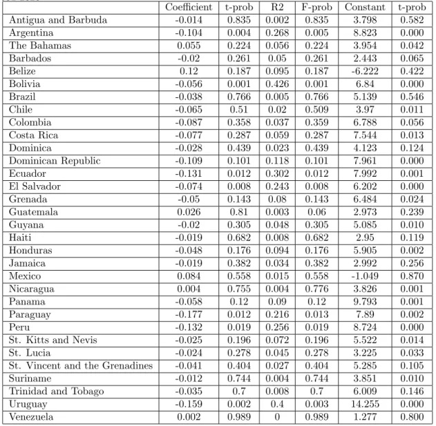
Table 12: Growth rate of output on debt gdp ratio in Latin America and Carrebean Countries, 1991-2020
Coe¢ cient t-prob R2 F-prob Constant t-prob
Antigua and Barbuda -0.014 0.835 0.002 0.835 3.798 0.582
Argentina -0.104 0.004 0.268 0.005 8.823 0.000 The Bahamas 0.055 0.224 0.056 0.224 3.954 0.042 Barbados -0.02 0.261 0.05 0.261 2.443 0.065 Belize 0.12 0.187 0.095 0.187 -6.222 0.422 Bolivia -0.056 0.001 0.426 0.001 6.84 0.000 Brazil -0.038 0.766 0.005 0.766 5.139 0.546 Chile -0.065 0.51 0.02 0.509 3.97 0.011 Colombia -0.087 0.358 0.037 0.359 6.788 0.056 Costa Rica -0.077 0.287 0.059 0.287 7.544 0.013 Dominica -0.028 0.439 0.023 0.439 4.123 0.124 Dominican Republic -0.109 0.101 0.118 0.101 7.961 0.000 Ecuador -0.131 0.012 0.302 0.012 7.992 0.001 El Salvador -0.074 0.008 0.243 0.008 6.202 0.000 Grenada -0.05 0.143 0.08 0.143 6.484 0.024 Guatemala 0.026 0.81 0.003 0.06 2.973 0.239 Guyana -0.02 0.305 0.048 0.305 5.085 0.010 Haiti -0.019 0.682 0.008 0.682 2.95 0.119 Honduras -0.048 0.176 0.094 0.176 5.905 0.002 Jamaica -0.019 0.382 0.034 0.382 2.992 0.256 Mexico 0.084 0.558 0.015 0.558 -1.049 0.870 Nicaragua 0.004 0.755 0.004 0.776 3.826 0.001 Panama -0.058 0.12 0.09 0.12 9.793 0.001 Paraguay -0.177 0.012 0.216 0.013 7.89 0.002 Peru -0.132 0.019 0.256 0.019 8.724 0.000
St. Kitts and Nevis -0.025 0.196 0.072 0.196 5.522 0.014
St. Lucia -0.024 0.278 0.045 0.278 3.225 0.033
St. Vincent and the Grenadines -0.041 0.404 0.027 0.404 5.285 0.105
Suriname -0.012 0.744 0.004 0.744 3.851 0.010
Trinidad and Tobago -0.035 0.7 0.008 0.7 6.009 0.146
Uruguay -0.159 0.002 0.4 0.003 14.255 0.000