Pick Your Contexts Well: Understanding Object-Sensitivity

(1)

Pick Your Contexts Well: Understanding Object-Sensitivity

The Making of a Precise and Scalable Pointer Analysis

Yannis Smaragdakis

Department of Computer Science,

University of Massachusetts, Amherst, MA 01003, USA and Department of Informatics, University of Athens, 15784, Greece [email protected]—[email protected]

Martin Bravenboer

LogicBlox Inc. Two Midtown Plaza Atlanta, GA 30309, USA [email protected]

Ondˇrej Lhot´ak

David R. Cheriton School of

Computer Science University of Waterloo Waterloo, ON N2L 3G1, Canada

[email protected]

Abstract

Object-sensitivity has emerged as an excellent context abstraction for points-to analysis in object-oriented languages. Despite its prac-tical success, however, object-sensitivity is poorly understood. For instance, for a context depth of 2 or higher, past scalable imple-mentations deviate significantly from the original definition of an object-sensitive analysis. The reason is that the analysis has many degrees of freedom, relating to which context elements are picked at every method call and object creation. We offer a clean model for the analysis design space, and discuss a formal and informal un-derstanding of sensitivity and of how to create good object-sensitive analyses. The results are surprising in their extent. We find that past implementations have made a sub-optimal choice of contexts, to the severe detriment of precision and performance. We define a “full-object-sensitive” analysis that results in significantly higher precision, and often performance, for the exact same con-text depth. We also introduce “type-sensitivity” as an explicit ap-proximation of object-sensitivity that preserves high context qual-ity at substantially reduced cost. A type-sensitive points-to analysis makes an unconventional use of types as context: the context types are not dynamic types of objects involved in the analysis, but in-stead upper bounds on the dynamic types of their allocator objects. Our results expose the influence of context choice on the quality of points-to analysis and demonstrate type-sensitivity to be an idea with major impact: It decisively advances the state-of-the-art with a spectrum of analyses that simultaneously enjoy speed (several times faster than an analogous object-sensitive analysis), scalabil-ity (comparable to analyses with much less context-sensitivscalabil-ity), and precision (comparable to the best object-sensitive analysis with the same context depth).

Categories and Subject Descriptors F.3.2 [Logics and Meanings of Programs]: Semantics of Programming Languages—Program Analysis

; D.3.1 [Programming Languages]: Formal Definitions and Theory—Semantics

General Terms Algorithms, Languages, Performance

Permission to make digital or hard copies of all or part of this work for personal or classroom use is granted without fee provided that copies are not made or distributed for profit or commercial advantage and that copies bear this notice and the full citation on the first page. To copy otherwise, to republish, to post on servers or to redistribute to lists, requires prior specific permission and/or a fee.

POPL’11, January 26–28, 2011, Austin, Texas, USA. Copyright c2011 ACM 978-1-4503-0490-0/11/01. . . $10.00

1. Introduction

Points-to analysis (or pointer analysis in our context) is one of the most fundamental static program analyses. Points-to analysis con-sists of computing a static abstraction of all the data that a pointer expression (or just a variable, without loss of generality) can point to during program run-time. The analysis forms the basis for practi-cally every other program analysis and is closely inter-related with mechanisms such as call-graph construction, since the values of a pointer determine the target of dynamically resolved calls, such as object-oriented dynamically dispatched method calls or functional lambda applications. By nature, the entire challenge of points-to analysis is to pick judicious approximations. Intractability lurks be-hind any attempt to track program control- or data-flow precisely. Furthermore, the global character and complicated nature of the analysis make it hard to determine how different analysis decisions interact with various language features. For object-oriented and functional languages, context-sensitivity is a general approach that achieves tractable and usefully high precision. Context-sensitivity consists of qualifying local program variables, and possibly (heap) object abstractions, with context information: the analysis collapses information (e.g., “what objects this method argument can point to”) over all possible executions that result in the same context, while separating all information for different contexts. Two main kinds of context-sensitivity have been explored: call-site sensitivity [18, 19] and object-sensitivity [13].

Ever since the introduction of object-sensitivity by Milanova et al. [13], there has been accumulating evidence [3, 7, 8, 10, 14] that it is a superior context abstraction for object-oriented programs, yielding high precision relative to cost. The success of object-sensitivity has been such that, in current practice, object-sensitive analyses have almost completely supplanted traditional call-site sensitive/kCFA analyses for object-oriented languages. This paper is concerned with understanding object-sensitivity in depth, for-malizing it conveniently, and exploring design choices that produce even more scalable and precise analyses than current practice.

What is object-sensitivity at a high level? Perhaps the easi-est way to describe the concept is by analogy and contrast to the better-known call-site sensitivity. A call-site sensitive/kCFA analy-sis uses method call-sites (i.e., labels of instructions that may call the method) as context elements. That is, in OO terms, the analysis separates information on local variables (e.g., method arguments) per call-stack (i.e., sequence of k call-sites) of method invocations that led to the current method call. Similarly, the analysis separates information on heap objects per call-stack of method invocations that led to the object’s allocation. For instance, in the code example below, a 1-call-site sensitive analysis (unlike a context-insensitive

(2)

analysis) will distinguish the two call-sites of methodfooon lines 7 and 9. This means that the analysis will treatfooseparately for two cases: that of its argument,o, pointing to anythingsomeobj1may point to, and that ofopointing to anythingsomeobj2may point to. class A { 1 void foo(Object o) { ... } 2 } 3 4 class Client { 5

void bar(A a1, A a2) { ...

6 a1.foo(someobj1); 7 ... 8 a2.foo(someobj2); 9 } 10 } 11

In contrast, object-sensitivity uses object allocation sites (i.e., labels of instructions containing anewstatement) as context ele-ments. (Hence, a better name for “object-sensitivity” might have been “allocation-site sensitivity”.) That is, when a method is called on an object, the analysis separates the inferred facts depending on the allocation site of the receiver object (i.e., the object on which the method is called), as well as other allocation sites used as con-text. Thus, in the above example, a 1-object-sensitive analysis will analyzefooseparately depending on the allocation sites of the ob-jects thata1anda2may point to. It is not apparent from the above fragment neither whethera1anda2may point to different objects, nor to how many objects: the allocation site of the receiver object may be remote and unrelated to the method call itself. Similarly, it is not possible to compare the precision of an object-sensitive and a call-site sensitive analysis in principle. In this example, it is not even clear whether the object sensitive analysis will examine all calls tofooas one case, as two, or as many more, since this de-pends on the allocation sites of all objects that the analysis itself computes to flow intoa1anda2.

Note that our above description has been vague: “the analysis separates ... facts depending on the allocation site of the receiver object ... as well as other allocation sites”. What are these “other allocation sites”? The first contribution of our paper consists of rec-ognizing that there is confusion in the literature regarding this topic. The original definition of object-sensitivity (see [13], Fig.6, p.12.) defines the context of a method call to be the allocation site of the receiver object obj, the allocation site of the allocator object (obj′₎

of obj, (i.e., the receiver object of the method that made the alloca-tion of obj), the allocaalloca-tion site of the allocator object of obj′, and so on. Nevertheless, subsequent “object-sensitive” analyses (e.g., [5, 8, 10, 20], among many) maintain the fundamental premise of using allocation sites as context elements, yet differ in which allo-cation sites are used. For instance, the 2-object-sensitive analysis in the Pframework [7, 9] uses as method context the allocation site of the receiver object and the allocation site of the caller object (i.e., an object of classClient, and notA, in our example).

In this paper, we offer a unified formal framework that captures the object-sensitive analyses defined in the literature and allows a deeper understanding of their differences. Additionally, we imple-ment an array of object-sensitive analyses and draw insights about how the choice of context relates to scalability and precision. We discover that the seemingly simple difference of how an analy-sis context is chosen results in large differences in precision and performance. We use the name full-object sensitivity to refer to (a slight generalization of) the original statement of object-sensitivity by Milanova et al. We argue that full-object sensitivity is an excel-lent choice in the design space, while the choice of context made in past actual implementations is sub-optimal and results in substan-tial loss of precision. Concretely, a practical outcome of our work is to establish a 2-full-object-sensitive analysis with a 1-object sen-sitive heap (shortened to “2full+1H”) as an analysis that is often

(though not always) feasible with current technology and impres-sively precise.

Perhaps even more importantly, our understanding of the impact of context on the effectiveness of an analysis leads to defining a new variant that combines scalability with good precision. Namely, we introduce the idea of a type-sensitive analysis, which is defined to be directly analogous to an object-sensitive analysis, yet approxi-mates (some) context elements using types instead of full allocation sites. In contrast to past uses of types in points-to analysis (e.g., [1, 15, 21] and see Ryder [17] for several examples) we demon-strate that the types used as contexts should not be the types of the corresponding objects. Instead, the precision of our type-sensitive analysis is due to replacing the allocation site of an object o (which would be used as context in an object-sensitive analysis) with an upper-bound of the dynamic type of o’s allocator object. The result is a substantial improvement that establishes a new sweet spot in the practical tradeoffof points-to analysis precision and performance.

In summary, our work makes the following contributions: •We offer a better understanding of the concept and variations

of object-sensitive points-to analyses. Our understanding relies on a precise formalism that captures the different object-sensitive analyses, as well as on informal insights.

•We identify the differences in past object-sensitive analyses and analyze the influence of these differences on precision and per-formance. We argue that full-object-sensitivity is a substantially better choice than others used in actual practice. We validate the impact of full-object-sensitivity for the case of a context depth of 2. The difference is significant in terms of precision and scalabil-ity. Our results help establish a 2full+1H analysis as the state-of-the-art for precision in object-oriented programs, among analyses that are often practically feasible.

•We introduce type-sensitivity, as a purposeful collapsing of the context information of an object-sensitive analysis, in order to improve scalability. We discuss what is a good type-sensitive context and show that the straightforward option (of replacing an object by its type) is catastrophically bad. Instead, we identify an excellent choice of type context and demonstrate that it yields a surprisingly ideal combination of precision and scalability. A type-sensitive analysis for a context depth of 2 is several times (2x to unboundedly high) faster than a corresponding object-sensitive analysis, while keeping almost the same precision. In fact, the run-time performance and scalability of a type-sensitive analysis often exceed those of a cheap object-sensitive analysis of a lower context depth, while yielding vastly more precision.

2. Formalizing Object-Sensitivity and Variations

We formalize analyses using an abstract interpretation over a sim-plified base language that closely captures the key operations that practical points-to analyses perform. For this, we use Feather-weight Java [6] in “A-Normal” form. A-Normal FeatherFeather-weight Java is identical to ordinary Featherweight Java, except that argu-ments to a function call must be atomically evaluable. For example, the bodyreturn f.foo(b.bar());becomesb1 = b.bar(); f1 = f.foo(b1); return f1;. This shift does not change the expressive power of the language or the nature of the analysis, but it simplifies the semantics and brings the language closer to the intermediate languages that practical points-to analysis implementations operate on. Our formalism is an imperative variant (with a call stack in-stead of continuations) of the corresponding formalism of Might, Smaragdakis and Van Horn [12], which attempts a unified treat-ment of control-flow analysis (in functional languages) and points-to analysis (in imperative/OO languages).

(3)

The grammar below describes A-Normal Featherweight Java. Some of the Featherweight Java conventions merit a reminder: A class declaration always names a superclass, and lists fields (dis-tinct from those in the superclass) followed by a single constructor and a list of methods. Constructors are stylized, always taking in as many parameters as total fields in the class and superclasses, and consisting of a call to the superclass constructor and assignment of the rest of the fields, all in order.

Class::=classCextendsC′{−−−−−→C′′ f;K→−M} K∈Konst::=C(C f−−−→){super(→−f′) ;−−−−−−−−−−−−−−−→this.f′′=f′′′;} M∈Method::=C m(C v−−−→){C v−−−−→;~s}

s∈Stmt::=v=e;ℓ|returnv;ℓ

e∈Exp::=v|v.f|v.m(→−v)|newC(→−v)|(C)v v∈Varis a set of variable names f∈FieldNameis a set of field names C∈ClassNameis a set of class names

m∈MethodCallis a set of method invocation sites

ℓ∈Labis a set of labels

Every statement has a label, to provide a convenient way of refer-encing program points. The function succ :Lab⇀Stmtyields the subsequent statement for a statement’s label.

2.1 Concrete Semantics

We express the semantics using a small-step state machine. Figure 1 contains the state space. A state consists of a statement, a data stack (for local variables), a store, a call-stack (recording, for each active method invocation, the statement to return to, the context to re-store, and the location that will hold the return value), and a current context. Following earlier work [12], our concrete semantics antici-pates abstraction in that variables and fields are mapped to context-sensitive addresses, and the store maps such addresses to objects. The purpose served by the concept of a context-sensitive address is to introduce an extra level of indirection (through the store). In the usual concrete semantics, every dynamic instance of a variable or field will have a different context, making context-sensitive ad-dresses extraneous. Nevertheless, the existence of the store makes it easy to collapse information from different program paths, as long as variables or fields map to the same context-sensitive address.1_In

addition to being a map from fields to context-sensitive addresses, an object also stores its creation context. There are two different kinds of context in this state space: a context for local (method) variables, and a heap context, for object fields. At a first approxi-mation, one can think of the two contexts as being the same sets. Any infinite sets can play the role of context. By picking specific context sets we can simplify the mapping from concrete to abstract, as well as capture the essence of object-sensitivity.

The semantics are encoded as a small-step transition relation (⇒) ⊆Σ×Σ, shown in Figure 2. There is one transition rule for each expression type, plus an additional transition rule to account for return. Evaluation consists of finding all states reachable from an initial state (typically a single call statement with an empty store and binding environment). We use standard functions cons, car, cdr, and first_n to construct and deconstruct lists/stacks. For

1_{To prevent misunderstandings, we note that the extra level of indirection is}

the only purpose of the store in our semantics. Specifically, our store is not intended for modeling the Java heap and our stack is not modeling the Java local variable stack (although it has similar structure, as it is a map over local variables). For instance, the store is used to also map local variables to actual values, which is the purpose of a Java stack.

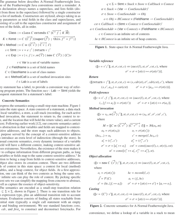
ς∈Σ =Stmt×Stack×Store×CallStack×Context st∈Stack=(Var⇀ContSensAddr)∗

σ∈Store=ContSensAddr→Obj

o∈Obj=HContext×(FieldName⇀ContSensAddr) cst∈CallStack=(Stmt×Context×ContSensAddr)∗ a∈ContSensAddr=(Var×Context)+(FieldName×HContext)

c∈Context is an infinite set of contexts hc∈HContext is an infinite set of heap contexts.

Figure 1. State-space for A-Normal Featherweight Java.

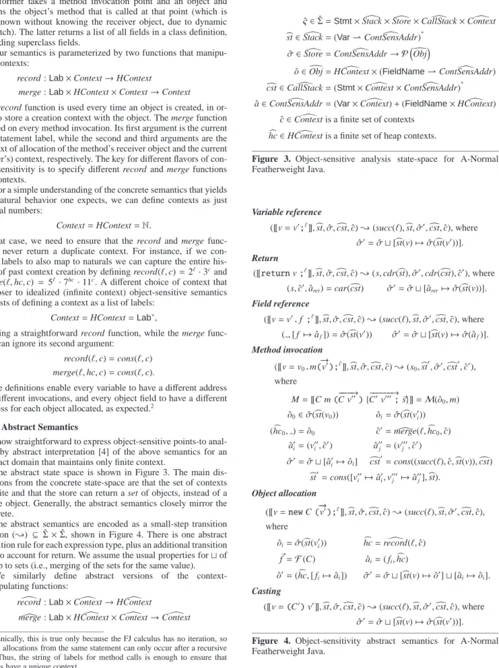
Variable reference ([[v=v′;ℓ]],st, σ,cst,c)⇒(succ(ℓ),st, σ′_, cst,c), where σ′₌_σ₊_[st(v)_7→_σ_(st(v′_))]. Return ([[returnv;ℓ]],st, σ,cst,c)⇒(s,cdr(st), σ′_,_cdr(cst)_,_c′_{), where}

(s,c′,aret)=car(cst) σ′=σ+[aret7→σ(st(v))].

Field reference ([[v=v′.f;ℓ]],st, σ,cst,c)⇒(succ(ℓ),st, σ′_, cst,c), where (,[ f 7→af])=σ(st(v′)) σ′=σ+[st(v)7→σ(af)]. Method invocation ([[v=v0.m( − → v′);ℓ]],st, σ,cst,c)⇒(s0,st′, σ′,cst′,c′), where M=[[C m(−−−−→C v′′₎_{_C−−−−−−→′_v′′′_;_~_s}_]]₌_M_(o 0,m) o0=σ(st(v0)) oi=σ(st(v′i)) (hc0, )=o0 c′=merge(ℓ,hc0,c) a′ i=(v ′′ i,c ′₎ _a′′ j =(v ′′′ j ,c ′₎ σ′₌_σ₊ [a′i 7→oi] cst′=cons((succ(ℓ),c,st(v)),cst) st′=cons([v′′i 7→a ′ i,v ′′′ j 7→a ′′ j],st). Object allocation ([[v=newC(→−v′_);ℓ ]],st, σ,cst,c)⇒(succ(ℓ),st, σ′_,_cst_,_c), where oi=σ(st(v′i)) hc=record(ℓ,c) ~ f=F(C) ai=( fi,hc) o′=(hc,[ fi7→ai]) σ′=σ+[st(v)7→o′]+[ai7→oi]. Casting ([[v=(C′)v′]],st, σ,cst,c)⇒(succ(ℓ),st, σ′_, cst,c), where σ′₌_σ₊_[st(v)_7→_σ_(st(v′_))].

Figure 2. Concrete semantics for A-Normal Featherweight Java.

convenience, we define a lookup of a variable in a stack to mean a lookup in the top component of the stack, e.g., st(v) means (car(st))(v). We also use helper functions

M: Obj×MethodCall⇀Method F :ClassName→FieldName∗.

(4)

The former takes a method invocation point and an object and returns the object’s method that is called at that point (which is not known without knowing the receiver object, due to dynamic dispatch). The latter returns a list of all fields in a class definition, including superclass fields.

Our semantics is parameterized by two functions that manipu-late contexts:

record :Lab×Context→HContext

merge :Lab×HContext×Context→Context

The record function is used every time an object is created, in or-der to store a creation context with the object. The merge function is used on every method invocation. Its first argument is the current call statement label, while the second and third arguments are the context of allocation of the method’s receiver object and the current (caller’s) context, respectively. The key for different flavors of con-text sensitivity is to specify different record and merge functions for contexts.

For a simple understanding of the concrete semantics that yields the natural behavior one expects, we can define contexts as just natural numbers:

Context=HContext=N.

In that case, we need to ensure that the record and merge func-tions never return a duplicate context. For instance, if we con-sider labels to also map to naturals we can capture the entire his-tory of past context creation by defining record(ℓ,c)=2ℓ_·₃c_and

merge(ℓ,hc,c) =5ℓ_·₇hc_·₁₁c_{. A di}_ff_{erent choice of context that}

is closer to idealized (infinite context) object-sensitive semantics consists of defining a context as a list of labels:

Context=HContext=Lab∗,

yielding a straightforward record function, while the merge func-tion can ignore its second argument:

record(ℓ,c)=cons(ℓ,c) merge(ℓ,hc,c)=cons(ℓ,c).

These definitions enable every variable to have a different address for different invocations, and every object field to have a different address for each object allocated, as expected.2

2.2 Abstract Semantics

It is now straightforward to express object-sensitive points-to anal-yses by abstract interpretation [4] of the above semantics for an abstract domain that maintains only finite context.

The abstract state space is shown in Figure 3. The main dis-tinctions from the concrete state-space are that the set of contexts is finite and that the store can return a set of objects, instead of a single object. Generally, the abstract semantics closely mirror the concrete.

The abstract semantics are encoded as a small-step transition relation ({) ⊆ Σˆ ×Σˆ, shown in Figure 4. There is one abstract transition rule for each expression type, plus an additional transition rule to account for return. We assume the usual properties for⊔of a map to sets (i.e., merging of the sets for the same value).

We similarly define abstract versions of the context-manipulating functions:

[

record :Lab×Context[ →HContext[

[

merge :Lab×HContext[ ×Context[ →Context[

2_{Technically, this is true only because the FJ calculus has no iteration, so}

object allocations from the same statement can only occur after a recursive call. Thus, the string of labels for method calls is enough to ensure that objects have a unique context.

ˆ

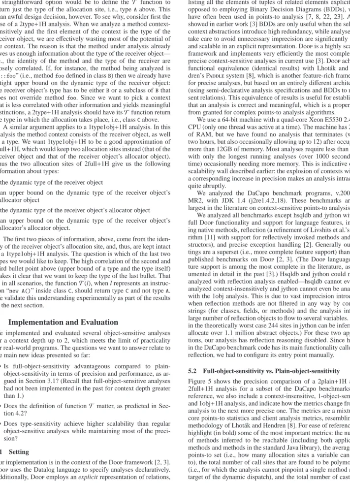
ς∈Σ =ˆ Stmt×Stack[ ×_Store[_×_CallStack[ _×_Context[ b

st∈Stack[ =(Var⇀_{ContSensAddr)}[ ∗

ˆ

σ∈Store[=ContSensAddr[ → PdObj

ˆo∈dObj=HContext[ ×(FieldName⇀ContSensAddr)[

c

cst∈CallStack[ =(Stmt×Context[ ×ContSensAddr)[ ∗ ˆa∈ContSensAddr[ =(Var×Context)[ +(FieldName×HContext)[

ˆc∈Context is a finite set of contexts[

b

hc∈HContext is a finite set of heap contexts.[

Figure 3. Object-sensitive analysis state-space for A-Normal

Featherweight Java. Variable reference ([[v=v′;ℓ]],bst,σ,ˆ ccst,ˆc){(succ(ℓ),bst,σˆ′,cstc,ˆc), where ˆ σ′₌_σ_ˆ _⊔_[_st(v)_b _7→_σ_ˆ₍_b_st(v′_))]. Return ([[returnv;ℓ]],stb,σ,ˆ cstc,ˆc){(s,cdr(bst),σˆ′,cdr(ccst),ˆc′), where (s,ˆc′_,_ˆa

ret)=car(cst)c σˆ′=σˆ ⊔[ˆaret7→σˆ(bst(v))].

Field reference ([[v=v′_._f _;ℓ ]],bst,σ,ˆ cstc,ˆc){(succ(ℓ),bst,σˆ′,ccst,ˆc), where (,[ f 7→âf])=σˆ(bst(v′)) σˆ′=σˆ ⊔[bst(v)7→σˆ(âf)]. Method invocation ([[v=v0.m( − → v′_);ℓ ]],bst,σ,ˆ cstc,ˆc){(s0,bst ′ ,σˆ′_,_cst_c′_,_ˆc′_), where M=[[C m(−−−−→C v′′){−−−−−−→C′v′′′;~s}]]=M( ô0,m) ô0∈σˆ(bst(v0)) ôi=σˆ(bst(v′i)) (hcb0, )=ô0 ˆc′=merge([ ℓ,hcb0,ˆc) â′ i=(v ′′ i,ˆc ′₎ _â′′ j =(v ′′′ j ,ˆc ′₎ ˆ σ′₌ ˆ σ⊔[â′i 7→ôi] ccst ′ =cons((succ(ℓ),ˆc,bst(v)),ccst) b st′=cons([v′′i 7→â ′ i,v ′′′ j 7→â ′′ j],bst). Object allocation ([[v=newC(→−v′_);ℓ ]],bst,σ,ˆ cstc,ˆc){(succ(ℓ),bst,σˆ′,ccst,ˆc), where ôi=σˆ(bst(vi′)) hcb=record([ ℓ,ˆc) ~ f =F(C) âi=( fi,hc)b ô′₌₍_hc_b_,_{[ f}

i7→âi]) σˆ′=σˆ ⊔[bst(v)7→ô′]⊔[âi7→ôi].

Casting ([[v=(C′)v′]],bst,σ,ˆ cstc,ˆc){(succ(ℓ),bst,σˆ′,ccst,ˆc), where ˆ σ′₌ ˆ σ⊔[bst(v)7→σˆ(bst(v′))].

Figure 4. Object-sensitivity abstract semantics for A-Normal

(5)

The abstract record and[ merge functions capture the essence of[

object-sensitivity: an object-sensitive analysis is distinguished by its storing a context together with every allocated object (via

[

record), and by its retrieving that context and using it as the basis for the analysis context of every method dispatched on the object (via_merge).[

2.3 Analysis Variations and Observations

With the above framework, we can concisely characterize all past object-sensitive analyses, as well as discuss other possibilities. All variations consist of only modifying the definitions of Context,[

[

HContext,record, and[ _merge.[

Original Object Sensitivity. Milanova et al. [13] gave the original definition of object-sensitivity but did not implement the analysis for context depths greater than 1. Taken literally, the original defi-nition prescribes that, for an n-object-sensitive analysis, the regular and the heap context consist of n labels:

[

Context=HContext[ =Labn,

whilerecord just keeps the first n elements of the context defined[ in our concrete semantics, and_{merge discards everything but the}[

receiver object context:

[

record(ℓ,ˆc)=cons(ℓ,first_n−1(ˆc))

[

merge(ℓ,hcb,ˆc)=hc.b

In practical terms, this definition has several consequences:

•_{The only labels used as context are labels from an object}

allo-cation site, via therecord function.[

•_{On a method invocation, only the (heap) context of the receiver}

object matters.

•_{The heap context of a newly allocated object is derived from the}

context of the method doing the allocation, i.e., from the heap context of the object that is doing the allocation.

In other words, the context used to analyze a method consists of the allocation site of the method’s receiver object, the allocation site of the object that allocated the method’s receiver object, the allocation site of the object that allocated the object that allocated the method’s receiver object, and so on. In the next section we discuss whether this is a good choice of context for scalability and precision.

Past Implementations of Object Sensitivity. For an object-sensitive analysis with context depth 1, the context choice is ob-vious. Themerge function has to use some of the receiver object[

context, or the analysis would not be object-sensitive (just call-site-sensitive), and the receiver object context consists of just the ob-ject’s allocation site.

For analyses with context depth n>1, however, the definitions ofmerge and[ record can vary significantly. Actual implementations[ of such analyses deviated from the Milanova et al. definition. No-tably, the Pframework [7, 9] (which provides the most-used such implementation available) merges the allocation site of the receiver object with multiple context elements from the caller ob-ject context when analyzing a method. This results in the following functions:

[

record(ℓ,ˆc)=cons(ℓ,first_n−1(ˆc))

[

merge(ℓ,hcb,ˆc)=cons(car(hc)b ,firstn−1(ˆc)).

The practically interesting case is of n=2. (Higher values are well outside current technology if the analysis is applied as defined, i.e., the context depth applies to all program variables.) The above defi-nition then means that every method is analyzed using as context a)

the allocation site of the receiver object; and b) the allocation site of the caller object.

Heap Context, Naming, and Full-Object Sensitivity. The above analyses defined the heap context (HContext) and the regu-[ lar/method context (Context) to be the same set, namely[ Labn_.

There are other interesting possibilities, however. Since themerge[

function has access to a heap context and to a regular context (and needs to build a new regular context) the heap context can be shal-lower. For instance, Lhot´ak’s exploration of object-sensitive analy-ses [7] studies in depth analyanaly-ses where the heap context is always just a single allocation site:

[ HContext=Lab [ Context=Labn [ record(ℓ,ˆc)=ℓ [

merge(ℓ,hcb,ˆc)=cons(hcb,first_n−1(ˆc)).

In fact, the above definition is what is most commonly called an “object-sensitive analysis” in the literature! The analyses we saw earlier are colloquially called “object-sensitive analyses with a context-sensitive (or object-sensitive) heap”. That is, the points-to analysis literature by convention uses context points-to apply only points-to methods, while heap objects are represented by just their allocation site. Adding more context to object fields than just the object al-location site is designated with suffixes such as “context-sensitive heap” or “heap cloning” in an analysis description. Thus, one needs to be very careful with naming conventions. We summarize ours at the end of this section.

Another interesting possibility is that of keeping a deeper con-text for heap objects than for methods. The most meaningful case in practice is the one where the heap object keeps one extra context element: [ HContext=Labn+1 [ Context=Labn [ record(ℓ,ˆc)=cons(ℓ,ˆc).

(Themerge function can vary orthogonally, as per our earlier dis-[

cussion.) For n=1, this is Lhot´ak’s “1obj+H” analysis, which is currently considered the best trade-offbetween scalability and pre-cision [8], and to which we refer repeatedly in our experimental evaluation of Section 5

This latest variation complicates naming even more. In Lhot´ak’s detailed naming scheme, the above analysis would be an “n-object-sensitive analysis with an (n-)object-“n-object-sensitive heap”, while our standard n-object-sensitive analysis (withContext[ =HContext[ = Labn) is called an “n-object-sensitive analysis with an n− 1-object-sensitive heap”. The reason for the off-by-one convention is his-torical: it is considered self-evident in the points-to analysis com-munity that the static abstraction for a heap object will consist of at least its allocation site label. Therefore, the heap context is con-sidered to be n−1 labels, when the static abstraction of an object consists of n labels in total.

In the rest of this paper, we adopt the standard terminology of the points-to analysis literature. That is, we talk of an “n-object-sensitive analysis with an n−1-object-sensitive heap” to mean that

[

Context=HContext[ =Labn_{. Furthermore, to distinguish between}

the two dominant definitions of amerge function (Milanova et al.’s,[

as opposed to that of the Pframework) we refer to a full-object-sensitive analysis vs. a plain-full-object-sensitive analysis. A full-object-sensitive analysis is characterized by amerge function:[

[

(6)

That is, the “full” object abstraction of the receiver object is used as context for the method invoked on that object. In contrast, a plain-object-sensitive analysis merges information from the receiver and the caller objects:

[

record(ℓ,ˆc)=cons(ℓ,firstn−1(ˆc))

[

merge(ℓ,hcb,ˆc)=cons(car(hc)b ,firstn−1(ˆc)).

Thus, the original object-sensitivity definition by Milanova et al. is a full-object-sensitive analysis, while the practical object-sensitive analysis of the Pframework is plain-object-sensitive. We ab-breviate plain-object-sensitive analyses for different context and heap context depths to “nplain+mH” and full-object-sensitive anal-yses to “nfull+mH”. When the two analyses coincide, we use the abbreviation “nobj+mH”.

Discussion. Finally, note that our theoretical framework is not limited to traditional object-sensitivity, but also encompasses call-site sensitivity. Namely, themerge function takes the current call-[

site label as an argument. None of the actual object-sensitive analy-ses we saw above use this argument. Thus, our framework suggests a generalized interpretation of what constitutes an object-sensitive analysis. We believe that the essence of object-sensitivity is not in “only using allocation-site labels as context” but in “storing an ob-ject’s creation context and using it at the site of a method invoca-tion” (i.e., the functionality of themerge function). We expect that[

future analyses will explore this direction further, possibly combin-ing call-site and allocation-site information in interestcombin-ing ways.

Our framework also allows the same high-level structure of an analysis but with different context information preserved. Section 4 pursues a specific direction in this design space, but generally we can produce analyses by using as context any abstractions com-putable from the arguments to functionsrecord and[ merge (with ap-[

propriate changes to theContext and[ HContext sets). For instance,[ we can use as context coarse-grained program location informa-tion (module identifiers, packages, user annotainforma-tions) since these are uniquely identified by the current program statement label,ℓ. Simi-larly, we can make different context choices for different allocation sites or call sites, by defining therecord and[ merge functions con-[

ditionally on the supplied label. In fact, there are few examples of context-sensitive points-to analyses that cannot be captured by our framework, and simple extensions would suffice for most of those. For instance, a context-sensitive points-to analysis that employs as context a static abstraction of the arguments of a method call (and not just of the receiver object) is currently not directly expressible in our formalism. (This approach has been fruitful in different static analyses, e.g., for type inference [1, 15].) Nevertheless, it is a sim-ple matter to adjust the form of themerge function and the “method[

invocation” rule in order to allow the method call context to also be a function of the heap contexts of argument objects.

3. Insights on Context Choice

With the benefit of our theoretical map of context choices for object-sensitivity, we next discuss what makes a scalable and pre-cise analysis in practice.

3.1 Full-Object-Sensitivity vs. Plain-Object-Sensitivity

The first question in our work is how to select which context ele-ments to keep—i.e., what is the best definition of themerge func-[

tion for practical purposes. We already saw the two main distinc-tions, in the form of full-object-sensitive vs. plain-object-sensitive analyses. Consider the standard case of a 2-object-sensitive anal-ysis with a 1-object-sensitive heap, i.e., per the standard naming convention,Context[ = HContext[ = Lab2_{. The 2full}₊_{1H analysis}

will examine every method using as context the allocation site of

the method’s receiver object, and the allocation site of the alloca-tor of this receiver object. (Recall that all information for method invocations under the same context will be merged, while informa-tion under different contexts will be kept separate.) In contrast the 2plain+1H analysis examines every method using as context the allocation site of the receiver object, and the allocation site of the caller object.

The 2full+1H analysis has not been implemented or evaluated in practice before. Yet with an understanding of how context is em-ployed, there are strong conceptual reasons why one may expect 2full+1H to be superior to 2plain+1H. The insight is that context serves the purpose of yielding extra information to classify dy-namic paths, at high extra cost for added context depth. Thus, for context to serve its purpose, it needs to be a good classifier, splitting the space of possibilities in roughly uniform partitions. When mix-ing context elements (allocation site labels) from the receiver and the caller object (as in the 2plain+1H analysis), the two context el-ements are likely to be correlated. High correlation means that a 2-object-sensitive analysis is effectively reduced to a high-cost 1-object-sensitive one. In a simple case of context correlation, an ob-ject calls another method on itself: the receiver obob-ject and the caller object are the same.3_{There are many more patterns of common}

ob-ject correlation—knowing that we are executing a method of obob-ject p almost always yields significant information about which object q is the receiver of a method call. Wrapper patterns, proxy pat-terns, the Bridge design pattern, etc., all have pairs of objects that are allocated and used together. For such cases of related objects, one can see the effect in intuitive terms: The traditional mixed con-text of a 2plain+1H analysis classifies method calls by asking ob-jects “where were you born and where was your sibling born?” A 2full+1H analysis asks “where were you born and where was your parent born?” The latter is a better differentiator, since birth loca-tions of siblings are more correlated.

3.2 Context Depth and Analysis Complexity

The theme of context element correlation and its effect on precision is generally important for analysis design. The rule of thumb is that context elements should be as little-correlated as possible for an analysis with high precision. To see this consider how context depth affects the scalability of an analysis. There are two opposing forces when context depth is increased. On the one hand, increased precision may help the analysis avoid combinatorial explosion. On the other hand, when imprecision will occur anyway, a deeper context analysis will be significantly less scalable.

For the first point, consider the question “when can an analysis with a deeper context outperform one with a shallower context?” Concretely, are there cases when a 2-object-sensitive analysis will be faster or more scalable than a 1-object-sensitive analysis (for otherwise the same analysis logic, i.e., both plain-obj or full-obj)? Much of the cost of evaluating an analysis is due to propagating matching facts. Consider, for instance, the “Variable reference” rule from our abstract semantics in Figure 4, which results in an evaluation of the form: ˆσ′ ₌ _σ_ˆ _⊔_[_b_st(v) _7→ _σ_ˆ₍_b_st(v′_{))]. For}

this evaluation to be faster under a deeper context, the lookup ˆ

σ(bst(v′_{)) should return substantially fewer facts, i.e., the analysis}

context should result in much higher precision. Specifically two conditions need to be satisfied. First, the more detailed context should partition the facts well: the redundancy should be minimal between partitions in context-depth-2 that would project to the same partition with context depth 1. Intuitively, adding an extra level of context should not cause all (or many) facts to be replicated

3_{This case can be detected statically by the analysis, and context repetition}

can be avoided. This simple fix alone is not sufficient for reliably reducing the imprecision of a 2plain+1H analysis, however.

(7)

for all (or many) extra context elements. Second, fewer facts should be produced by the rule evaluation at context depth 2 relative to depth 1, when compared after projection down to depth-1 facts. In other words, going to context depth 2 should be often enough to tell us that some object does not in fact flow to a certain 1-context-sensitive variable, because the assignment is invalid given the more precise context knowledge.

In case of imprecision, on the other hand, the deeper context will almost always result in a combinatorial explosion of the pos-sible facts and highly inefficient computation. When going from a 1obj+H analysis to a 2full+H or 2plain+H, we have every fact an-alyzed in up to N times more contexts (where N is the total number of context elements, i.e., allocation sites). As a rule of thumb, ev-ery extra level of context can multiply the space consumption and runtime of an analysis by a factor of N, and possibly more, since the N-times-larger collections of facts need to be used to index in other N-times-larger collections, with indexing mechanisms (and possibly results) that may not be linear.

It is, therefore, expected that an analysis with deeper context will perform quite well when it manages to keep precise facts, while exploding in runtime complexity when the context is not sufficient to maintain precision. Unfortunately, there are inevitable sources of imprecision in any real programming language—these include reflection (which is impossible to handle soundly and precisely), static fields (which defeat context-sensitivity), arrays, exceptions, etc. When this imprecision is not well-isolated and affects large parts of a realistic program, the points-to analysis will almost cer-tainly fail (within any reasonable time and space bound). This pro-duces a scalability wall effect: a given analysis on a program will either terminate quickly or will fail to terminate “ever” (in practi-cal terms). Input characteristics of the program (e.g., size metrics) are almost never good predictors of whether the program will be easy to analyze, as this property depends directly on the induced analysis imprecision.

The challenge then becomes whether we can maintain high precision while reducing the possibility for a combinatorial blowup of analysis facts due to deeper context. We next introduce a new approach in this direction.

4. Type-Sensitivity

If an analysis with a deeper context by nature results in a combina-torial explosion in complexity, then a natural step is to reduce the base of the exponential function. Context elements in an object-sensitive analysis are object allocation sites, and typical programs have too many allocation sites, making the product of the number of allocation sites too high. Therefore, a simple idea for scalability is to use coarser approximations of objects as context, instead of complete allocation sites. This would collapse the possible combi-nations down to a more manageable space, yielding improved scal-ability. The most straightforward static abstraction that can approx-imate an object is a type, which leads to our idea of a type-sensitive analysis.

4.1 Definition of Type-Sensitive Analysis

A type-sensitive analysis is almost identical to an object-sensitive analysis, but whereas an object-sensitive analysis would keep an allocation site as a context element, a type-sensitive analysis keeps a type instead.4_{Consider, for instance, a 2-type-sensitive analysis}

with a 1-type-sensitive heap (henceforth “2type+1H”). The method context for this analysis consists of two types. (For now we do not care which types. We discuss later what types yield high precision.)

4_{Despite the name similarity, our type-sensitive points-to analysis has no}

relationship to Reppy’s “type-sensitive control-flow analysis” [16], which uses types to filter control flow facts in a context-insensitive analysis.

Expressed in our framework, the 2type+1H analysis has:

[

HContext=Lab×ClassName

[

Context=ClassName2.

Note again the contrast of the standard convention of the points-to analysis community and the structure of abstractions: the 2type+1H analysis also includes an allocation site label in the static abstrac-tion of an object—this aspect is considered so essential that it is not reflected on the analysis name. Approximating the allocation site of the object itself by a type would be possible, but detrimental for precision.

Generally, type-contexts and object-contexts can be merged at any level, as long as themerge function can be defined. An in-[

teresting choice is an analysis that merely replaces one of the two allocation sites of 2full+1H with a type, while leaving all the rest of the context elements intact. We call this a 1-type-1-object-sensitive analysis with a 1-object-sensitive heap, and shorten the name to “1type1obj+1H”. That is, a 1type1obj+1H analysis has:

[

HContext=Lab2

[

Context=Lab×ClassName.

The 2type+1H and the 1type1obj+1H analyses are the most practically promising type-sensitive analyses with a context depth of 2. Their context-manipulation functions can be described with the help of an auxiliary function

T :Lab→ClassName,

which retrieves a type from an allocation site label. For 2type+1H, the context functions become:5

[ record(ℓ,ˆc=[C1,C2])=[ℓ,C1] [ merge(ℓ,hcb =[ℓ′_, C],ˆc)=[T(ℓ′ ),C], while for 1type1obj+1H, the two functions are:

[ record(ℓ,ˆc=[ℓ′_, C])=[ℓ, ℓ′ ] [ merge(ℓ,hcb =[ℓ1, ℓ2],ˆc)=[ℓ1,T(ℓ2)],

In other words, the two analyses are variations of 2full+1H (and not of 2plain+1H), with some of the context information down-graded to be types instead of allocation site labels. The functionT makes opaque the method we use to produce a type from an allo-cation site, which we discuss next.

4.2 Choice of Type Contexts

Just having a type as a context element does not tell us how good the context will be for ensuring precision—the choice of type is of paramount importance. The essence of understanding what consti-tutes a good type context is the question “what does an allocation site tell us about types?” After all, we want to use types as a coarse approximation of allocation sites, so we want to maintain most of the information that allocation sites imply regarding types.

The identity of an allocation site, i.e., an instruction “new A()” inside classC, gives us:

•the dynamic typeAof the allocated object

•an upper boundCon the dynamic type of the allocator object. (Since the allocation site occurs in a method of class C, the allocator object must be of typeCor a subclass of Cthat does not override the method containing the allocation site.)

5_{We use common list and pattern-matching notation to avoid long}

expres-sions. E.g., “record([ ℓ,ˆc=[C1,C2])” means “when the second argument, ˆc,

(8)

A straightforward option would be to define the T function to return just the type of the allocation site, i.e., typeAabove. This is an awful design decision, however. To see why, consider first the case of a 2type+1H analysis. When we analyze a method context-sensitively and the first element of the context is the type of the receiver object, we are effectively wasting most of the potential of the context. The reason is that the method under analysis already gives us enough information about the type of the receiver object— i.e., the identity of the method and the type of the receiver are closely correlated. If, for instance, the method being analyzed is “B::foo” (i.e., methodfoodefined in classB) then we already have a tight upper bound on the dynamic type of the receiver object: the receiver object’s type has to be eitherBor a subclass ofBthat does not override methodfoo. Since we want to pick a context that is less correlated with other information and yields meaningful distinctions, a 2type+1H analysis should have itsT function return the type in which the allocation takes place, i.e., classCabove.

A similar argument applies to a 1type1obj+1H analysis. In this analysis the method context consists of the receiver object, as well as a type. We want 1type1obj+1H to be a good approximation of 2full+1H, which would keep two allocation sites instead (that of the receiver object and that of the receiver object’s allocator object). Thus the two allocation sites of 2full+1H give us the following information about types:

•the dynamic type of the receiver object

•an upper bound on the dynamic type of the receiver object’s allocator object

•the dynamic type of the receiver object’s allocator object •an upper bound on the dynamic type of the receiver object’s

allocator’s allocator object.

The first two pieces of information, above, come from the iden-tity of the receiver object’s allocation site, and, thus, are kept intact in a 1type1obj+1H analysis. The question is which of the last two types we would like to keep. The high correlation of the second and third bullet point above (upper bound of a type and the type itself) makes it clear that we want to keep the type of the last bullet. That is, in all scenarios, the functionT(l), when l represents an instruc-tion “new A()” inside classC, should return typeCand not typeA. We validate this understanding experimentally as part of the results of the next section.

5. Implementation and Evaluation

We implemented and evaluated several object-sensitive analyses for a context depth up to 2, which meets the limit of practicality for real-world programs. The questions we want to answer relate to the main new ideas presented so far:

•Is full-object-sensitivity advantageous compared to plain-object-sensitivity in terms of precision and performance, as ar-gued in Section 3.1? (Recall that full-object-sensitive analyses had not been implemented in the past for context depth greater than 1.)

•_{Does the definition of function}_T _{matter, as predicted in}

Sec-tion 4.2?

•_{Does type-sensitivity achieve higher scalability than regular}

object-sensitive analyses while maintaining most of the preci-sion?

5.1 Setting

Our implementation is in the context of the Dframework [2, 3]. Duses the Datalog language to specify analyses declaratively. Additionally, Demploys an explicit representation of relations,

listing all the elements of tuples of related elements explicitly, as opposed to employing Binary Decision Diagrams (BDDs), which have often been used in points-to analysis [7, 8, 22, 23]. As we showed in earlier work [3] BDDs are only useful when the selected context abstractions introduce high redundancy, while analyses that take care to avoid unnecessary imprecision are significantly faster and scalable in an explicit representation. Dis a highly scalable framework and implements very efficiently the most complex and precise context-sensitive analyses in current use [3]. Dachieves functional equivalence (identical results) with Lhot´ak and Hen-dren’s Psystem [8], which is another feature-rich framework for precise analyses, but based on an entirely different architecture (using semi-declarative analysis specifications and BDDs to repre-sent relations). This equivalence of results is useful for establishing that an analysis is correct and meaningful, which is a property far from granted for complex points-to analysis algorithms.

We use a 64-bit machine with a quad-core Xeon E5530 2.4GHz CPU (only one thread was active at a time). The machine has 24GB of RAM, but we have found no analysis that terminates (within two hours, but also occasionally allowing up to 12) after occupying more than 12GB of memory. Most analyses require less than 2GB, with only the longest running analyses (over 1000 seconds run time) occasionally needing more memory. This is indicative of the scalability wall described earlier: the explosion of contexts without a corresponding increase in precision makes an analysis intractable quite abruptly.

We analyzed the DaCapo benchmark programs, v.2006-10-MR2, with JDK 1.4 (j2re1.4.2 18). These benchmarks are the largest in the literature on context-sensitive points-to analysis.

We analyzed all benchmarks except hsqldb and jython with the full Dfunctionality and support for language features, includ-ing native methods, reflection (a refinement of Livshits et al.’s algo-rithm [11] with support for reflectively invoked methods and con-structors), and precise exception handling [2]. Generally our set-tings are a superset (i.e., more complete feature support) than prior published benchmarks on D [2, 3]. (The D language fea-ture support is among the most complete in the literafea-ture, as doc-umented in detail in the past [3].) Hsqldb and jython could not be analyzed with reflection analysis enabled—hsqldb cannot even be analyzed context-insensitively and jython cannot even be analyzed with the 1obj analysis. This is due to vast imprecision introduced when reflection methods are not filtered in any way by constant strings (for classes, fields, or methods) and the analysis infers a large number of reflection objects to flow to several variables. (E.g., in the theoretically worst case 244 sites in jython can be inferred to allocate over 1.1 million abstract objects.) For these two applica-tions, our analysis has reflection reasoning disabled. Since hsqldb in the DaCapo benchmark code has its main functionality called via reflection, we had to configure its entry point manually.

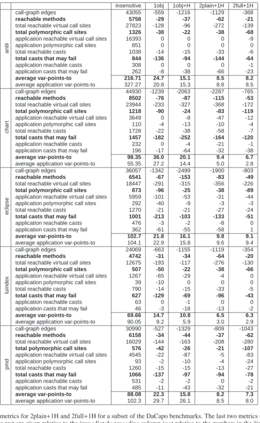
5.2 Full-object-sensitivity vs. Plain-object-sensitivity

Figure 5 shows the precision comparison of a 2plain+1H and a 2full+1H analysis for a subset of the DaCapo benchmarks. For reference, we also include a context-insensitive, 1-object-sensitive and 1obj+1H analysis, and indicate how the metrics change from an analysis to the next more precise one. The metrics are a mixture of core points-to statistics and client analysis metrics, resembling the methodology of Lhot´ak and Hendren [8]. For ease of reference, we highlight (in bold) some of the most important metrics: the number of methods inferred to be reachable (including both application methods and methods in the standard Java library), the average var-points-to set (i.e., how many allocation sites a variable can refer to), the total number of call sites that are found to be polymorphic (i.e., for which the analysis cannot pinpoint a single method as the target of the dynamic dispatch), and the total number of casts that

(9)

insensitive 1obj 1obj+H 2plain+1H 2full+1H a n tl r call-graph edges 43055 -559 -1216 -1129 -368 reachable methods 5758 -29 -37 -62 -21

total reachable virtual call sites 27823 -128 -96 -272 -139

total polymorphic call sites 1326 -38 -22 -38 -68

application reachable virtual call sites 16393 0 0 0 -9 application polymorphic call sites 851 0 0 0 0 total reachable casts 1038 -14 -15 -33 -6

total casts that may fail 844 -136 -94 -144 -64

application reachable casts 308 0 0 0 -1 application casts that may fail 262 -8 -38 -66 -23

average var-points-to 216.71 24.7 15.1 8.5 8.2

average application var-points-to 327.27 20.8 15.3 8.8 8.5

c h a rt call-graph edges 44930 -1239 -2063 -2287 -765 reachable methods 8502 -76 -87 -115 -53

application reachable virtual call sites 3649 0 -8 -47 -12 application polymorphic call sites 110 -4 -13 -10 -4 total reachable casts 1728 -22 -38 -58 -7

application reachable casts 232 0 -4 -21 -1 application casts that may fail 196 -17 -64 -32 -38

e c lip s e call-graph edges 36057 -1342 -2499 -1900 -803 reachable methods 6541 -67 -153 -83 -49

application reachable virtual call sites 5959 -101 -53 -31 -44 application polymorphic call sites 292 -40 -9 -3 -3 total reachable casts 1270 -21 -21 -27 -24

application reachable casts 476 -3 -2 -8 0 application casts that may fail 362 -61 -55 -58 1

lu in d e x call-graph edges 24069 -663 -1155 -1119 -354 reachable methods 4742 -31 -34 -64 -20

application reachable virtual call sites 1267 -65 -29 -4 0 application polymorphic call sites 39 -10 0 0 0 total reachable casts 790 -14 -15 -33 -5

application reachable casts 63 0 -1 0 0 application casts that may fail 46 -3 -18 -13 -2

p

m

d

call-graph edges 30990 -527 -1329 -809 -1043

reachable methods 6158 -34 -44 -37 -62

application reachable virtual call sites 4545 -22 -87 -5 -83 application polymorphic call sites 93 -2 -10 -4 -24 total reachable casts 1260 -15 -15 -13 -27

application reachable casts 531 -2 -2 0 -2 application casts that may fail 485 -11 -43 -32 -21

Figure 5. Precision metrics for 2plain+1H and 2full+1H for a subset of the DaCapo benchmarks. The last two metrics (“average ...”) are in absolute numbers, the rest are given relative to the immediately preceding column (not relative to the numbers in the “insensitive” column). All metrics are end-user (i.e., context-insensitive) metrics. Var-points-to is the main relation of a points-to analysis, linking a variable to the allocation sites it may be referring to. (The average is over variables.) “Reachable methods” is the same as call-graph nodes, hence the first two metrics show how precise is the on-the-fly inferred call-graph. “Polymorphic call-sites” are those for which the analysis cannot statically determine a unique receiver method. “Casts that may fail” are those for which the analysis cannot statically determine that they are safe.

(10)

may fail at run-time (i.e., for which the analysis cannot statically determine that the cast is always safe). These metrics paint a fairly complete picture of relative analysis precision, although the rest of the metrics are useful for framing (e.g., for examining how the statistics vary between application classes and system libraries, for comparing to the total number of reachable call sites, etc.).

As can be seen in Figure 5, 2full+1H is almost always signif-icantly more precise than 2plain+1H, even though both analyses have the same context depth. The difference in precision is quite substantial: For several metrics and programs (e.g., multiple met-rics for pmd, or reduction in total polymorphic virtual call sites for many programs), the difference between full-object-sensitivity and plain-object-sensitivity is as large as any other single-step incre-ment in precision (e.g., from 1-obj to 1obj+H).

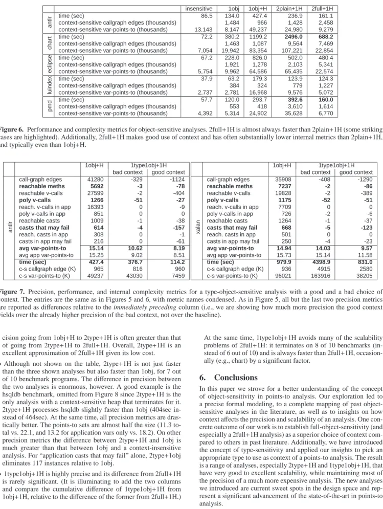
Perhaps most impressively, this precision is accompanied by substantially improved performance. Figure 6 shows the running time of the analyses, together with two key internal complexity metrics: the number of edges in the context-sensitive callgraph (i.e., how many context-qualified methods are inferred to call how many other qualified methods) and the size of the context-sensitive var-points-to set, i.e., the total number of facts inferred that relate a context-qualified variable with a context-qualified al-location site.

The running time of 2full+1H is almost always much lower than that of 2plain+1H. The case of “chart” is most striking, with 2full+1H finishing in well under a third of the time of 2plain+1H, while achieving the much higher precision shown in Figure 5. The internal metrics show that 2full+1H makes excellent use of its context and has substantially lower internal complexity than 2plain+1H. Note that the statistics for context-sensitive var-points-to are quite low, explaining why the analysis is faster, since each variable needs to be examined only in a smaller number of contexts. A second reason why such internal metrics are important is that the performance of an analysis depends very much on algorithmic and data structure implementation choices, such as whether BDDs are used to represent large relations. Internal metrics, on the other hand, are invariant and indicate a complexity of the analysis that often transcends representation choices.

It is easy to see from the above figures that full-object-sensitivity makes a much better choice of context than plain-object-sensitivity, resulting in both increased precision and better perfor-mance. In fact, we have found the 2full+1H analysis to be a sweet spot in the current set of near-feasible analyses in terms of preci-sion. Adding an extra level of context sensitivity for object fields, yielding a 2full+2H analysis, adds extremely little precision to the analysis results while greatly increasing the analysis cost.

In fact, for the benchmarks shown, 2full+1H is even signifi-cantly faster than the much less precise 1obj+H. Nevertheless, the same is not true universally. Of the 10 DaCapo benchmarks in our evaluation set, 2full+1H handles 6 with ease (the 5 shown plus “lusearch” which has very similar behavior to “luindex”) but its running time explodes for the other 4. The 2plain+1H analysis ex-plodes at least as badly for the 4 benchmarks, but a 1obj+H anal-ysis handles 9 out of 10, and a 1-obj analanal-ysis handles all of them. In short, the performance (and internal complexity) of a highly-precise but deep-context analysis is bimodal: when precision is maintained, the analysis performs admirably. When, however, sig-nificant imprecision creeps in, the analysis does badly, since the number of contexts increases in combinatorial fashion.

Therefore, 2full+1H achieves excellent precision but is not a good point in the design space in terms of scalability. (In the past, the only fully scalable uses of object-sensitivity with depth> 1 have applied deep context to a small, carefully selected subset of allocation sites; we are interested in scalability when the whole

program is analyzed with the precision of deep context.) This is the shortcoming that we expect to address with type-sensitive analyses.

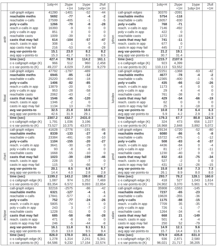
5.3 Importance of Type Context Choice

In Section 4.2 we argued that, for judicious use of the extra con-text element, functionT has to be defined so that it returns the enclosing type of an allocation site and not the type that is be-ing allocated. Experimentally, this is very clearly the case. Fig-ure 7 demonstrates this for two of our benchmark programs (the alphabetically first and last, which are representative of the rest). 1obj+H is shown as a baseline, to appreciate the difference. With the “wrong” type context, a 1type1obj+1H analysis is far more ex-pensive and barely more precise than 1obj+H, while with the right type context the analysis is impressively scalable and precise (very close to 2full+1H, as we show later).

As can be seen, the impact of a good context is highly signif-icant, both for scalability (in terms of time and internal metrics) and for precision. In our subsequent discussion we assume that all type-sensitive analyses use the superior context, as defined above.

5.4 Type-Sensitivity Precision and Performance

We found that type-sensitivity fully meets its stated goal: it yields analyses that are almost as precise as full-object-sensitive ones, while being highly scalable. In fact, type-sensitive analyses seem to clearly supplant other current state-of-the-art analyses—e.g., both 2type+1H and 1type1obj+1H seem overwhelmingly better than 1obj+H in both precision and performance for most of our benchmarks and metrics.

Our experiment space consists of the four precise analyses that appear feasible or mostly-feasible with current capabilities: 1obj+H, 2type+1H, 1type1obj+1H, and 2full+1H. Figure 8 shows the results of our evaluation for 8 of the 10 benchmark programs. (There is some replication of numbers compared to the previous ta-bles, but this is limited to columns included as baselines.) We omit lusearch for layout reasons, since it behaves almost identically to luindex. We discuss the final benchmark, hsqldb, in text, but do not list it on the table because 2type+1H is the only of the four analyses that terminates on it.

Note that the first two analyses (1obj+H, 2type+1H) are seman-tically incomparable in precision but every other pair has a prov-ably more precise analysis, so the issue concerns the amount of extra precision obtained and the running time cost. Specifically, 2full+1H is guaranteed to be more precise than the other three anal-yses, and 1type1obj+1H is guaranteed to be more precise than ei-ther 1obj+H or 2type+1H.

The trends from our experiments are quite clear:

•Although there is no guarantee, 2type+1H is almost always more precise than 1obj+H, hence the 2type+1H precision metrics (re-ported in the table relative to the preceding column, i.e., 1obj+H) are overwhelmingly showing negative numbers (i.e., an improve-ment). Additionally, 2type+1H is almost always (for 9 out of 10 programs) the fastest analysis in our set. In all but one case, 2type+1H is several times faster than 1obj+H—e.g., 5x faster or more for 4 of the benchmarks. The clear improvement of 2type+1H over 1obj+H is perhaps the most important of our ex-perimental findings. Recall that 1obj+H is currently considered the “sweet spot” of precision and scalability in practice: a highly precise analysis, that is still feasible for large programs without exploding badly in complexity.

•2type+1H achieves great scalability for fairly good precision. It is the only analysis that terminates for all our benchmark pro-grams. It typically produces quite tight points-to sets, with antlr being a significant exception that requires more examination. In terms of client analyses and end-user metrics, the increase in