CHAPTER 14 D
ATA
A
NALYSIS
S
OFTWARE FOR
I
ON
B
EAM
A
NALYSIS
Handbook of Modern Ion Beam Analysis, 2nd Edition, eds. Yongqiang Wang and
Michael Nastasi, Materials Research Society, Warrendale 2010 (2009), pp 305-345.
N. P. Barradas
Instituto Tecnológico e Nuclear, Sacavém, Portugal
Centro de Física Nuclear da Universidade de Lisboa, Lisboa, Portugal
E. Rauhala
University of Helsinki, Helsinki, Finland
CONTENTS
14.1 INTRODUCTION... 14.1.1 Data analysis software... 14.1.2 Scope of the chapter... 14.1.3 Historical development and reviews of software programs... 14.2 TYPES OF CODES... 14.2.1 The direct calculation method... 14.2.2 Simulation by successive iterations... 14.2.3 Interactive versus automated... 14.2.4 Deterministic versus stochastic (Monte Carlo)... 14.3 CAPABILITIES OF CODES... 14.3.1 Design basis... 14.3.1.1. Techniques implemented... 14.3.1.2. Experimental conditions supported... 14.3.1.3. Description of samples... 14.3.2 Databases implemented... 14.3.2.1. Stopping power... 14.3.2.2. Scattering cross section... 14.3.3 Basic physics... 14.3.4 Advanced physics... 14.3.4.1. Straggling models... 14.3.4.2. Electron screening... 14.3.4.3. Plural scattering... 14.3.4.4. Multiple scattering... 14.3.4.5. Simulation of resonances... 14.3.4.6. Surface and interface roughness... 14.3.4.7. Channeling... 14.3.4.8. Pulse pileup...
14.3.5.2. Bayesian inference... 14.3.6 Usability and usage... 14.4 ACCURACY... 14.4.1 Numerical accuracy of codes... 14.4.2 Intrinsic accuracy of IBA experiments... 14.4.2.1. Models and basic physical quantities... 14.4.2.2. Experimental conditions... 14.4.2.3. Counting statistics... 14.4.3 Physical effects on data analysis... 14.5 RUMP AND FIRST-GENERATION CODES... 14.6 NEW-GENERATION CODES: SIMNRA AND NDF... 14.6.1 Further capabilities... 14.6.2 SIMNRA... 14.6.3 NDF... 14.6.4 Issues... 14.7 MONTE CARLO SIMULATION... 14.8 OTHER TECHNIQUES... 14.8.1 PIXE... 14.8.2 Resonant NRA, PIGE, NRP, MEIS, channeling, microscopies, and so
on
14.9 THE IBA DATA FORMAT IDF... ACKNOWLEDGEMENTS... SOFTWARE WEB SITES... REFERENCES...
14.1 INTRODUCTION 14.1.1 Data analysis software
The data analysis software in ion beam methods are computer programs designed to extract information about samples from the measured ion beam spectra. The desired information includes identification of sample elements, their concentrations, areal densities, and layer thicknesses. At best, one spectrum can be converted to concentration–depth distributions of all elements in the sample. Often, however, such a full description of the sample based on a single experiment is not possible. The analyst can then perform additional experiments using different experimental parameters such as ion energies or a different measurement geometry or including information from one or more other complementary techniques.
The software can also be used for designing relevant experiments. Depending on the assumed sample structure, the appropriate ion beam technique can be chosen by doing test simulations prior to experiments. For example, the most suitable parameters for the measurements can be tested. The choice of ions, energies, geometries, and so on can be examined without performing often extensive and complicated experiments.
The third main function of the software is found in education and research. By using simulation computer programs, the researcher can readily scrutinize the characteristics of various ion beam techniques. The dependencies between stopping powers, cross sections, energies, and so on can be studied. Novel reaction cross sections and stopping powers can be implemented in the programs to investigate the agreement between simulation and experimental data. Fine details, such as double and multiple scattering, screening, pileup, and the properties of various detector systems can be analyzed with the help of data analysis programs.
It cannot be overemphasized that software is an aid to data analysis and does not replace the judgment of the analyst. Software that is not correctly used, or that is used outside its scope of application, leads to wrong data analysis. Furthermore, it should be noted that the scope of application of a given program might not be clear and will depend on the details of the experiment being analyzed: for instance, Bohr straggling is adequate for analysis of normal-incidence proton Rutherford backscattering spectrometry (RBS) with a surface barrier detector, but it is completely inadequate for heavy-ion elastic recoil detection analysis (ERDA) or for high-resolution near-surface analysis, where the straggling is asymmetric.
14.1.2 Scope of the chapter
This chapter deals mainly with the data analysis software of particle–particle ion beam analysis (IBA) techniques: Rutherford backscattering spectrometry (RBS), elastic recoil detection analysis (ERDA), and nuclear reaction analysis (NRA). In the last case, we limit ourselves to techniques utilizing one single beam energy, as opposed to resonant NRA or narrow resonance profiling (NRP) [see Amsel (1996) for a discussion on acronyms]. Short sections on particle-induced X-ray emission (PIXE) spectroscopy and other techniques such as NRP and channeling are also included.
A list of Web sites relevant for IBA software and data analysis is provided at the end of the chapter, just before the list of references. Note that this list is by no means
14.1.3 Historical development and reviews of software programs
Computer programs to analyze data from RBS, NRA, and ERDA date back to the 1960s and 1970s. These techniques developed in parallel with the beginning of the new semiconductor and other high-technology industries, where new needs for ion beams in the production, modification, and characterization of novel materials were arising. IBA techniques for quantitative depth profiling in the micron range and determination of low-concentration elemental impurities were quickly recognized and widely applied. As these analytical tools became more versatile, the samples, spectra, and data analysis problems also became more complicated. By the end of the 1990s, the collection of software had developed in various directions: codes exist that can handle very general data analysis problems and various IBA techniques; some are highly automatic, whereas others treat specified problems with great exactness.
The historical development of the software was reviewed recently by Rauhala et al.
(2006), which presents the characteristics and status of 12 software packages as of 2006. An intercomparison of several software packages for simulations and real data-analysis
applications is presented in Barradas et al. (2007b). Relevant developments up to 2009
are also included in this chapter. 14.2 TYPES OF CODES
14.2.1 The direct calculation method
In direct spectrum analysis, the yields from separated signals of the spectrum are transformed into concentration values by closed-form analytical calculation. Other forms of direct analysis include conversion from signal areas and heights to total amounts or concentrations. This is the opposite of spectrum simulation, where a theoretical spectrum is generated from an assumed depth profile and compared to the actual data.
This approach was introduced by Børgesen et al. (1982) with the code SQUEAKIE.
This approach is straightforward and effective in many cases. However, it has problems because of the implementation of straggling and the stability of results as a result of uncertainties in the stopping database and measurement noise. The direct method is still used, normally as a complement to full simulations, and often in heavy-ion ERDA (Spaeth et al., 1998).
14.2.2 Simulation by successive iterations
Almost all of the presently available IBA data analysis software is based on simulation by successive iterations. The simulation modeling assumes that the underlying physics, mathematics, and nuclear and atomic data are valid and adequately describe the physical processes involved. Starting from a known sample structure, the corresponding experimental energy spectrum can be theoretically simulated from a few basic data and the known formalism of the reaction spectrometry. by comparing the experimental and theoretical spectra and iteratively modifying the assumed composition of the sample, a close similarity of the spectra is typically accomplished after a few iterations. The sample structure leading to the theoretical spectrum is then taken to correspond to the material’s sample structure. Erroneous results or misinterpretations of the material’s
structure can result from incorrect science, ambiguous data, or inadequate software documentation and guidance for analysts to extract the correct information.
The typical iterative simulation proceeds as follows:
1. Assume the experimental parameters and the known experimental spectrum. 2. Assume an initial sample composition.
3. Calculate a theoretical spectrum corresponding to the experimental parameters and the assumed sample composition.
4. Compare the simulated spectrum to the experimental spectrum.
5. Identify the differences and modify the assumed sample composition accordingly. 6. Repeat iteration steps 3–5 until an adequate fit between the simulated and experimental spectra is accomplished.
7. Take the sample parameters corresponding to the best simulation to be the sample structure resulting from the data analysis.
This procedure is illustrated in EXAMPLE 14.1.
______________________________________________________________________
EXAMPLE 14.1. Convergence of iteration.
Assume that the experimental parameters and the elements in the sample are known. Start by making a guess about the sample composition. How do the iterations converge?
Figure 14.1 shows the spectrum for 2.00 MeV 4He ions incident on a LaGaO layer on a silicon substrate. In the experiment, the following parameters were used:
Incident 4He-ion energy, EHe = 2.00 MeV
Scattering angle, θ = 170° Angle of incidence, θ1 = 50°
Solid angle × accumulated charge, QΩ = 69.0 msr µC
Energy per channel, δE = 3.475 keV/channel
Energy in zero channel, = 27.3 keV
Zeroth iteration: Initially, as a guess of the LaGaO film composition, equal concentrations of the elements in a layer of 200 × 1015 at./cm2 areal density were assumed.
Initial assumptions:
Equal amounts of the three elements, 33% La, 33% Ga, 33% O. Layer areal density, 200 × 1015 at./cm2.
⇒ 0thiteration.
The resulting simulated spectrum is denoted as the 0thiteration in Fig. 14.1. The
simulated signal heights of La and Ga and the signal width of La were then compared to those of the experimental spectrum. Concentrations and layer areal density were
changed assuming the same linear dependence between the signal heights and concentrations and between the signal widths and areal density of the layer.
The La concentration was thus multiplied by the ratio of the experimental La signal height to the simulated La signal height. Similarly, the areal density of the film was multiplied by the ratio of the experimental La signal width to the simulated La signal width.
This process was then repeated. The solid lines denoted as 1st, …, 4th, in Fig. 14.1, show the results of subsequent iterations. In detail, the iteration converged as follows: First iteration. The height of the experimental La signal was observed to be roughly 75% of the height of the simulated signal. The same ratio for Ga was observed to be 80%.
The experimental La signal was observed to be roughly 2.4 times wider than the simulated signal.
Reduce the La concentration to 75% × 0.33 = 0.25.
Reduce the Ga concentration to 80% × 0.33 = 0.26.
Increase the areal density of the layer to 2.4 × 200 × 1015 at./cm2 = 480 × 1015 at./cm2. ⇒ 1st iteration.
Second iteration. The height of the experimental La signal was observed to be 85% of the height of the simulated signal. The same ratio for Ga was observed to be 88%. The experimental signal was observed to be 1.2 times wider than the simulated signal.
Reduce the La concentration to 85% × 0.25 = 0.21.
Increase the areal density of the layer to 1.2 × 480 × 1015 at./cm2 = 580 × 1015 at./cm2.
⇒ 2nd iteration.
Third iteration. The height of the experimental La signal was observed to be 95% of the height of the simulated signal. The same ratio for Ga was observed to be 93%. The experimental signal was observed to be 1.06 times wider than the simulated signal.
Reduce the La concentration to 95% × 0.21 = 0.20.
Reduce the Ga concentration to 93% × 0.23= 0.21.
Increase the areal density of the layer to 1.06 × 580 × 1015 at./cm2 = 615 × 1015 at./cm2. ⇒ 3rd iteration.
Fourth iteration. The height of the experimental La signal was observed to be 97% of the height of the simulated signal. The fit of the Ga signal was acceptable.
The experimental signal was observed to be 1.04 times wider than the simulated signal.
Reduce the La concentration to 97% × 0.20 = 0.195.
Maintain the Ga concentration at 0.21.
Increase the areal density of the layer to 1.04 × 615 × 1015 at./cm2 = 640 × 1015 at./cm2. ⇒ 4th iteration.
As a result of the fourth iteration, both the signal heights and the signal widths of La and Ga seem to be fitted adequately within the plotting accuracy of the figure. In practical terms, users tend to adjust the concentration and thickness values manually, without doing the exact procedure shown here. This leads to a larger number of iterations, which most users find acceptable given that the calculations are very fast with modern
computers.
______________________________________________________________________
The crucial point in the iterative procedure is to describe the sample composition. Several codes let the user introduce functions that describe the depth profile of a given element. However, the most popular method to describe a sample is to divide it into sublayers. Each sublayer has a different composition, which is iteratively changed. Also, the number of sublayers is increased or decreased during the iterative procedure: If the current number of layers is not sufficient to reproduce the changing signals observed, the user introduces a new layer. If, on the other hand, the user can obtain an equivalent fit by using fewer layers, this is normally preferred. In practice, the depth resolution of the experiment limits the number of layers needed. This is illustrated in EXAMPLE 14.2.
______________________________________________________________________
EXAMPLE 14.2. Simulating composition changes by division into sublayers.
Changes of concentrations of components within a layer can be treated by dividing the layer into sublayers of constant composition. Figure 14.2 shows a spectrum for 2.75
film and the substrate is not well defined and that the concentrations change with depth within the thin film.
This spectrum has been simulated by assuming nine sublayers of constant composition. The simulated spectrum as a result of data analysis by the program GISA is illustrated as the thick solid line connecting the experimental data points. The theoretical signals of the elemental components in each of the sublayers are shown as thin solid lines. The thick solid line thus represents the sum of the thin lines of the elemental signals in the sublayers.
The experimental parameters, the concentrations of the elements, and the areal densities of the sublayers are given in Table 14.1. The concentrations of the elements versus areal density are shown in Fig. 14.3.
FIG. 14.2. Backscattering spectrum for 2.75 MeV 7Li ions incident on a PbZrSnO thin-film sample on a Si substrate. The thick solid line connecting the experimental data points is the simulated spectrum. FIG. 14.3. The constant
concentrations of the elements (see Table 14.1) versus areal density. Table 14.1. Experimental
parameters and concentrations of
Incident particle 7Li, E0 = 2750 keV, δE = 4.424 keV/channel, QΩ = 9.687 µC msr, scattering angle 165°, angle of incidence 60°, exit angle 45°, system resolution 25 keV full width at half-maximum (fwhm).
Sublayer 1015 at./cm2 Pb Sn Zr Si O 1 100 0.16 0.0075 0.145 0 0.6875 2 100 0.173 0.0128 0.163 0 0.6512 3 100 0.168 0.0155 0.165 0 0.6515 4 50 0.17 0.019 0.1 0.1 0.611 5 50 0.11 0 0.022 0.31 0.558 6 50 0.036 0 0.0153 0.66 0.2887 7 50 0.023 0 0 0.977 0 8 200 0.0015 0 0 0.9985 0 9 5000 0 0 0 1 0
None of the layers was assumed to contain any undetected light elements. The oxygen signal was not fitted; the oxygen concentration follows from the concentrations of the heavier elements, as it is presumed to make up the total fractional concentration of each sublayer to 1. Bohr straggling and a scaled stopping of 1.08 times the TRIM-91 stopping value were assumed for the metal oxide layers.
The example is intended to demonstrate how the composition variations can be treated as constant composition sublayers. As discussed in Section 14.3.4.6, the interdiffusion and interfacial roughness can usually not be distinguished by using a backscattering spectrometry. In the present case, the probable cause for the mixing of the elements at the interface is diffusion, as the atomic-layer deposition of the metal oxide film should not change the smooth Si surface.
______________________________________________________________________
14.2.3 Interactive versus automated
The iterative procedure can be executed in an interactive way, where the user repeatedly refines the depth profile until it is considered that better agreement cannot be reached within the time and patience limits of the user; or with an automated process based on
optimization of some target function such as a χ2 or likelihood function.
Caution is needed when using automated optimization. Different depth profiles can lead to the same simulated spectrum (Butler, 1990), and the code has no way of knowing which of the possible solutions is the correct one. The user must often restrict the solution space, for instance, by performing only a local optimization on a limited number of parameters, one at a time.
A second problem is that the χ2 function is very sensitive to the quality of the simulation: for instance, if straggling is not included, an automated procedure will return interfacial mixing layers that might not exist. This can be solved naturally by including straggling, but there are some physical effects for which no accurate
processes will lead to artifacts in the depth profiles derived, unless the user restricts the solution space to physical solutions.
In any case, some form of automation is desirable, particularly if large quantities of data are to be analyzed.
14.2.4 Deterministic versus stochastic (Monte Carlo)
Deterministic codes follow a calculational procedure that is defined a priori. In
simulations, the sample is divided into thin sublayers. Both the incoming beam energy and the detected energy for scattering on each element present are calculated for each sublayer. The simulation is then constructed based on these quantities and on the concentration of each element in each sublayer. Straggling and other physical phenomena can be included. However, individual collisions between the analyzing ion (and its electrons) and the target nuclei and electrons are not modeled.
These deterministic simulations are normally very fast, lending themselves very well to the interactive and automated procedures described above, and they are, in fact, the standard approach.
Monte Carlo codes work in a completely different, more fundamental, way. They model individual interactions between particles. In this way, phenomena that have traditionally been difficult to include in the standard method are included in a natural way. The quality of the simulations that can be reached is, in principle, much superior.
However, there are issues with the calculation times required. Even with modern computers, acceleration techniques to speed up the calculations must be used. These include, for instance, disregarding collisions with scattering angles smaller or larger
than values defined a priori and artificially increasing the scattering cross section or the
solid angle of the detector in order to have more events. In some cases, such techniques can affect the quality of the simulations.
A second issue is related to the fact that Monte Carlo codes often require very detailed knowledge about the physics involved, and so far, their use has remained mostly confined to the code authors. Until recently, almost all data analysis was performed using deterministic codes (the largest exception was the use of Monte Carlo codes for the analysis of channeling data).
Nevertheless, improvements of the calculation times, coupled with the development of user-friendly interfaces, mean that Monte Carlo codes are becoming more widespread and might become dominant in areas such as heavy-ion ERDA, where multiple scattering and special detection systems play a large role.
14.3 CAPABILITIES OF CODES
In this section, we discuss some of the considerations that are important when selecting an IBA code. We note that there is no such thing as a “best code” for all situations. All codes discussed here do well at what they were designed to do, as shown by an intercomparison exercise organized by the International Atomic Energy Agency (IAEA)
(Barradas et al., 2007b). No code is complete in the sense that it can analyze all possible
IBA data.
The codes that took part in the IAEA intercomparison exercise were compared numerically and validated. Some of their most important characteristics are shown in
(2006). We stress that all information given was valid at the time of writing, as several codes are being actively developed.
When choosing which code to use, users must consider whether a given code is capable of extracting the information required and how easy it is to do so with each code. A complex sample where interface roughness and multiple scattering play a crucial role might need a last-generation code, but to determine the thickness of a thin film with one single heavy element on a light substrate, a full Monte Carlo calculation is probably too much work without extra benefit. Also, in some cases, manual calculations with careful consideration of error sources might be the most accurate method (see, for instance, Boudreault et al., 2002).
14.3.1 Design basis
The first consideration is obviously whether the data to be analyzed are within the design basis of the code considered. The two main points are the techniques implemented by each code and, for each technique, the experimental conditions supported.
For instance, if a code can only analyze RBS data with H and He beams, there is no point in trying to use it to analyze NRA data, but it might be possible to adapt it to analyze RBS with heavier ions, particularly if the source code is available.
In a similar way, even if a code includes RBS, for example, it might be limited to given experimental conditions. One example is the detection geometry: some codes include not only the well-known IBM and Cornell geometries, but also general geometry where any location of the detector is allowed (including transmission). Another consideration is the detection system, with most codes including only energy-dispersive systems, whereas some can include velocity and time-of-flight spectra, magnetic spectrometers, and others.
14.3.1.1 Techniques implemented
As stated in Section 14.1.2, this chapter is aimed predominantly at RBS and ERDA software packages. Elastic backscattering spectrometry (EBS) is, in practice, RBS with non-Rutherford cross sections that must be provided by the user (or included in the code) for each given ion/target nucleus pair.
Nonresonant NRA is also included here because it also uses one single beam energy (as opposed to resonant NRA, where the energy is scanned), and it is common that both the scattered beam and some reaction product are detected simultaneously.
Techniques such as channeling, PIXE, and resonant NRA are included in some of the codes.
Table 14.6 lists the techniques implemented in each code. All implement RBS, but some do not include ERDA or NRA. The code NDF is the only one to include PIXE. Note, however, that some laboratories perform only RBS, and it might be convenient to use a code with fewer options (and thus possibly easier to use) that can do what the user needs and nothing else. However, most laboratories employ several techniques, and using the same code to analyze all of the data has obvious advantages.
Table 14.6 also includes the experimental conditions supported by each code. They are similar for all codes, which handle most situations. Some differences exist, however, and users who need special conditions should consider carefully the varying capabilities of the codes. Also, it might be possible to convince authors of codes still under development to implement some specific experimental conditions not previously covered. If the source code is available, expert users can modify the supported experimental conditions according to their convenience.
14.3.1.3 Description of samples
One of the most important points in codes is how conveniently the sample can be described. This is illustrated in Table 14.8.
Homogeneous layers are considered in all codes that participated in the IAEA intercomparison exercise and in almost all codes known to us. In some codes, functions describing continuous profiles can also be introduced, which is important if, for instance, diffusion of implant profiles are being analyzed.
Sometimes, a maximum number of layers or of elements within a given layer is imposed. When restrictions on the number of layers exist, problems can arise when a very thin layer description is required. This is the case for samples with many thin layers and for high-resolution experiments (for instance, using a magnetic spectrometer or grazing-angle geometry).
RBS spectra are ambiguous whenever more elements are present than spectra were collected (Butler, 1990; Alkemade et al., 1990). In that case, more than one different depth profile can lead to exactly the same simulated spectrum. To remove ambiguities, more spectra should be collected, with different experimental conditions. However, often, the elements are bound in molecules, allowing the analyst to relate the respective signals to each other; for instance, if SiO2 is present, the small O signal can be related to the much larger Si signal by imposing the known stoichiometry. One very useful function in a code is therefore to allow the user to use as logical fitting elements not only atomic species, but molecules as well. The molecules can be of known or unknown composition. In the latter case, such a code would fit the molecular stoichiometry together with its concentration in each layer. One example of such an approach is discussed in Chapter 15, Pitfalls in Ion Beam Analysis.
In Fig. 14.4, we show the RBS spectra of a 21-layer ZrO2/SiO2 antireflection coating with a top Au layer (Jeynes et al., 2000a). The Zr had a small (known) amount of Hf
contamination. Both normal incidence and a 45° angle of incidence were used. The O,
Si, and Hf signals are small and superimposed on the much larger Zr signal. It is virtually impossible to analyze these data meaningfully without introducing the chemical information in some way. Consequently, the two spectra were fitted simultaneously, with the known molecules imposed as logical fitting elements. The small ~5% misfits might be due to inaccurate stopping or small deviations from stoichiometry. In any case, complete disambiguation of the data is achieved.
14.3.2 Databases implemented
One of the main conclusions of the IAEA intercomparison exercise of IBA softwares was that the greatest differences in the results arise from differences in the fundamental databases used, namely, the stopping-power database, as well as the non-Rutherford database in the case of EBS, ERDA, and NRA.
In the past decade, important advances have been made in terms of both new and more accurate experimental data and new theoretical and semiempirical schemes. Which databases are included in each code, as well as the possibility of loading new values, is thus an important factor.
14.3.2.1 Stopping power
The greatest advances in the knowledge of stopping power achieved in the past decade were for heavy ions. This was possible because of a wealth of new experimental data becoming available, which was integrated, for example, into both the most widely used stopping-power semiempirical interpolating scheme used in IBA work, SRIM (Ziegler, 2004; Ziegler et al., 2008), and MSTAR (Paul and Schinner, 2001, 2002), a program that calculates stopping powers for heavy ions. See Chapter 2 for further information on
100 200 300 400 0 2000 4000 0 2000 4000 6000 a) 0º Y ie ld ( c o u n ts ) Channel Zr Au Si O Y ie ld ( c o u n ts ) Channel Zr Au Si O b) 45º
FIG 14.4. Data and fit (solid line) obtained for a 21-layer ZrO2/SiO2 antireflection
coating with a top Au layer, shown for the data collected at (a) normal and (b) 45º incidence. The fitted partial spectra for Si and O are also shown.
For instance, in Fig. 14.5, we show the calculated spectrum for a 3 MeV 7Li beam impinging normally on a Si/SiO2 (2 × 10¹⁸ at./cm2)/Ti (1.5 × 10¹⁸ at./cm2) sample and detected at 160º, as obtained using 1985 stopping-power values and SRIM version 2006.02. It is clear that the very large changes in the simulation will be reflected in the accuracy of analyses of real data, with errors of up to 10% being made in thickness values, depending on the stopping values used.
500 1000 1500 0 50 100 150 200 O in SiO2 Y ie ld ( a rb . u n it s ) E (keV) ZBL85 SRIM 2006-02 Ti Si in SiO2 Si bulk
3 MeV 7Li on Si/SiO2 2x10¹⁸ at/cm2/Ti 1.5x10¹⁸ at/cm2
FIG. 14.5. Calculated spectra for 3 MeV 7Li beam incident on a Si/SiO2 sample. The only difference between the simulations is that different stopping powers were used: values from 1985 (solid line) and the most recently available values (dashed line). for accurate analyses, users must be aware of the stopping powers used by data analysis codes.
Large changes also occurred for light ions in some common systems. For instance, the stopping of He in Si is now known with an accuracy of better than 2%, and this update has been integrated into SRIM and other databases.
Also, many experiments in insulating compounds have shown that the Bragg rule does not always reproduce the experimental stopping, and the capability of including molecular stopping powers in codes is very important.
The stopping power along crystalline directions is usually smaller than that in a random direction or in an amorphous material with the same composition.
Ideally, codes should include the most recent stopping-power databases available, as well as the possibility of loading new stopping values for particular systems. In any
case, the users of data analysis software must be aware of the stopping used in a given analysis, along with its implications for the accuracy of the results obtained.
14.3.2.2 Scattering cross section
When analyzing EBS or NRA data, or 4He ERDA measurements of hydrogen isotopes,
for example, the non-Rutherford cross section used is of paramount importance. Some codes, namely SIMNRA, include a wide database of cross-section values for given ion/target pairs, whereas others read in external data files with the required cross sections.
The code SigmaCalc (Gurbich, 1997, 1998, 2005) for calculating cross sections from tabulated theoretical model parameters was developed by A. Gurbich. SigmaCalc is usually very reliable for those ion/target pairs that it includes, and it allows one to interpolate for scattering angles for which no measured cross sections are available. This action has also led to the integration of NRABASE and SIGMABASE into a single database called IBANDL (Ion Beam Analysis Nuclear Data Library), under the auspices of the IAEA.
Data with slowly changing non-Rutherford cross sections can be analyzed manually, as shown, for instance, in Chapter 5, section 5.3.4 of the first edition of this handbook
(Tesmer and Nastasi, 1995) for 4He ERDA analysis of hydrogen in Si3N4(H). However,
this is a painstaking procedure that can be done much faster, and more accurately, by computer simulation.
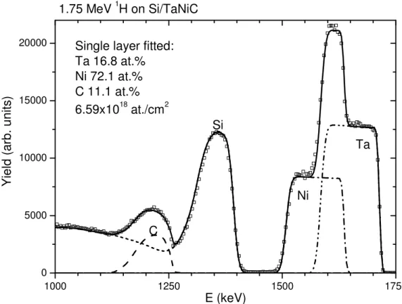
When superimposed signals with fast-changing cross sections are present, it becomes almost impossible to analyze the data manually, and computer codes must be used, along with the appropriate cross sections. For example, in Fig. 14.6, we show 1.75 MeV 1
H backscattering off a TaNiC film on Si (Jeynes et al., 2000b). The C signal is superimposed on the Si background, and both signals change rapidly because of the presence of resonances in both cross sections. The simulation includes one single homogeneous TaNiC layer and is the result of an automated fit that took less than 1 min. The scattering cross sections for C and Si were taken from SigmaCalc, and those for Ta and Ni are screened Rutherford cross sections.
1000 1250 1500 1750 0
5000 10000 15000
20000 Single layer fitted: Ta 16.8 at.% Ni 72.1 at.% C 11.1 at.% 6.59x10¹⁸ at./cm2 Ni Y ie ld ( a rb . u n it s ) E (keV) Ta Si C 1.75 MeV 1H on Si/TaNiC
FIG. 14.6. Spectrum for 1.75 MeV 1H backscattering off a TaNiC film on Si.
14.3.3 Basic physics
All IBA codes (except the Monte Carlo ones) employ similar principles to perform a basic simulation. The ingoing beam follows a straight trajectory, while losing energy, toward the sample; it interacts with a target nucleus; and the outgoing beam follows a straight trajectory, while losing energy, on its way to the detector. The energy spread of the beam (often called straggling) is also calculated.
From the point of view of the user, the fact that the different codes implement these steps in very different ways is not important.
The user wants to know, first, that all codes perform good simulations (at least for simple everyday spectra; complex samples might require particular codes). Confirming that a code is correct would imply a deep analysis of the physics included and of its implementation in the algorithms employed. Users do not want to do this, and often, they cannot (either because the source code is not available or because they do not have the time or the necessary background). Until recently, users simply assumed that codes were correct.
The IAEA intercomparison exercise showed that all of the analyzed codes produced
similar results for a 1.5 MeV 4He RBS simulation of a simple sample. Signal total yields
and signal heights were calculated with a 0.1–0.2% standard deviation between codes (as long as the same stopping powers and scattering cross sections were used in all cases). This is thus the error due to the differences in implementation of the same physics. It is smaller than the typical experimental errors coming, for example, from
counting statistics (rarely better than 1%) and much smaller than the error in the stopping-power values.
With the assurance that the codes (at least those that participated in the IAEA intercomparison) are correct for simple cases, the user might be concerned with how fast the simulations are. With modern computers, the simulation of simple spectra, even with straggling included, is always fast. Efficiency becomes important only when some further physics, such as plural scattering, is included.
14.3.4 Advanced physics
Although all simulation codes treat basic ion stopping and scattering phenomena, many of the subtle features in spectra arise from more complex interactions. The main issues involve energy spread, multiple and plural scattering, the handling of non-Rutherford cross sections, surface and interface roughness, and channeling.
The first comment is that, in principle, the best way of dealing with all of these phenomena is full Monte Carlo simulations. MCERD, for instance, is a Monte Carlo code for the analysis of ERDA data, but it can also handle RBS. It can include all of these effects, except for channeling. Different codes have been dedicated to the analysis of channeling in specific systems.
However, MC codes are mostly used by their authors, and calculation times can be an issue. Development of intuitive user interfaces and continuing gains in efficiency might change this situation, but for the moment, traditional codes are still the most often used. The following discussion is therefore related to traditional codes
We are concerned with determining the situations in which the basic simulations discussed in Section 14.3.3 are adequate. In situations where they are not adequate, we want to know whether codes include enough further physics to lead to meaningful analysis. The capabilities of the different codes are summarized in Table 14.7.
14.3.4.1 Straggling models
Practically all of the IBA codes implement the Bohr model (Bohr, 1948); with or
without the Chu/Yang correction (Chu, 1976; Yang et al., 1991), important for He and
heavier beams; some also implement the Tschalär effect (Tschalär, 1968a, 1968b; Tschalär and Maccabee, 1970), which is important in thick layers (for instance, to calculate the energy spread in a buried layer or after a stopper foil). Some codes let the user scale the calculated straggling. We note that pure Bohr straggling (without the Tschalär effect) is valid in a rather narrow range of energy loss, typically when the energy loss does not exceed around 20% of the initial beam energy.
However, straggling is important only if the detailed signal shape carries relevant information. To determine the stoichiometry and thickness of films, straggling is very often irrelevant, and the user can either ignore it or adjust the straggling to match observed signal widths. In this case, all codes are adequate.
If, on the other hand, interdiffusion or roughness between layers is being studied, or if a changing depth profile must be derived with maximum achievable accuracy, then any error in the straggling will directly lead to an error in the results. In such situations, the best available theory (i.e., a code that implements it) must be used.
State-of-the-art calculations of straggling, including geometrical straggling and multiple scattering, are performed by the code DEPTH (Szilágyi et al., 1995; Szilágyi, 2000). The recently presented RESOLNRA code (Mayer 2008) leads to equivalent results. No code dedicated to general-purpose IBA data analysis implements accurate straggling functions such as the Landau–Vavilov function. See, for instance, Bichsel (2006) and references therein for a detailed discussion of this issue.
The codes NDF and SIMNRA implement or are developing asymmetric straggling functions that might not be physically correct but that do represent reality better than the usual Gaussian distributions.
14.3.4.2 Electron screening
Electron screening at low energies decreases the effective charge of the target nucleus
seen by the analyzing ion, leading to a smaller scattering cross section (L'Ecuyer et al.,
1979;Andersen et al., 1980). It is greater for heavier target species and heavier ions, as
well as for lower energies. For 1.5 MeV 4He RBS off gold, it leads to a 2% correction to
the cross section. Most codes implement this effect. 14.3.4.3 Plural scattering
Plural scattering involves a few large-angle scattering events. It leads to a low-energy background, to an increased yield of bulk signals at low energies, and potentially to yield above the surface energy. Plural scattering can normally be disregarded, even when it is sizable, because it changes slowly with energy, and ad hoc backgrounds or signal subtraction techniques are often used.
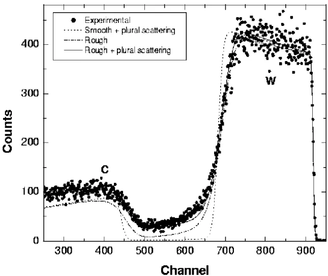
Plural scattering is important on the rare occasions where the yield at low energies or in a given background region must be understood quantitatively. Also, at grazing angle (of incidence or detection), it can make a large contribution even to the signal of fairly thin surface films. Both SIMNRA (Eckstein and Mayer, 1999) and NDF (Barradas, 2004) can calculate double scattering (two large-angle events, which accounts for most plural scattering). The two algorithms are not equivalent, but they lead to similar results in most situations. In some cases, such as in grazing-angle geometries, large differences might be observed, so the user should study the respective literature. Calculations are slow and not as accurate as for single scattering, but excellent reproduction of observed signals can be obtained, as seen in Fig. 14.7 (Mayer, 2002) for a normal incidence spectrum.
FIG. 14.7. 2.5 MeV protons backscattered from a 3.5-µm W layer on a rough carbon substrate, at normal incidence and with a scattering angle 165°. (Circles) Experimental data, (dotted line) calculated spectrum for a smooth W layer (3.6 µm) on a smooth C substrate including plural scattering, (dashed line) calculated spectrum for a rough W layer (3.5 µm, σ = 0.30 µm) on a rough substrate (fwhm 20°); (solid line) same as dashed line but including plural scattering. (From Mayer, 2002.).
14.3.4.4 Multiple scattering
Multiple scattering involves a large number of low-angle scattering events. It changes the trajectories of the beam ions, making them quite different from straight lines. This has many consequences, some of which standard codes are unable to calculate. It is therefore critical to know when it is important and when its effects can be calculated adequately.
Multiple scattering leads to an extra contribution to the energy spread of the beam, a change in the shape of signals because this contribution is not Gaussian-shaped, and a change in the observed yield.
It is more important for heavier ions at lower energies in heavier targets, as well as for grazing angles. In fact, at near-normal incidence, for the detection of ions with energies
At grazing angles (for instance, in ERDA), multiple scattering is often the most important contribution to energy spread. If energy spread is important (see Section 14.3.4.1), then multiple scattering must be calculated.
The best available calculations of multiple scattering (but not necessarily the best simulation of energy spectra) are made by the code DEPTH (Szilágyi et al., 1995). Some codes implement the extra energy spread, but assume it to be Gaussian-shaped. Most codes do not calculate multiple scattering. For heavy ions at fairly low velocities in grazing-angle geometries, none of the standard codes compares very well with Monte Carlo calculations, as of the time this was written.
14.3.4.5 Simulation of resonances
It is quite difficult to simulate buried sharp resonances. The combination of “buried” and “sharp” means whenever the energy spread of the beam before scattering is comparable to the resonance width. For bulk signals, the shape of the resonance signal is considerably affected; for thin films, the actual yield is also affected. This is important whenever a sharp resonance is used to enhance the yield from a buried element.
For instance, for protons crossing a 4.2-µm Ni film (leading to a high energy spread) on
top of a 1-µm Mylar film, the calculated C yield from the Mylar can be wrong by a factor of 10 if the energy spread of the beam is not taken into account (see Fig. 10 of Barradas et al., 2006).
To the best of our knowledge, the only code for analysis of general RBS and ERDA data that is currently able to calculate correctly the shape and yield in the presence of buried sharp resonances is NDF (Barradas et al., 2006). Dedicated codes for specific
systems (Tosaki et al., 2000) and for resonant NRA (Vickridge and Amsel, 1990; Pezzi
et al., 2005) also exist.
14.3.4.6 Surface and interface roughness
There is no general definition of roughness. Many different types of roughness exist. In the context of IBA, the most important point is that, in general, RBS experiments are not sufficient to determine which type of roughness is present. In fact, they are not even capable of distinguishing between layer interdiffusion and interfacial roughness. In almost all cases, extra information from other techniques [usually transmission electron microscopy (TEM) or atomic force microscopy (AFM)] is required. That said, RBS can be very useful for quantifying roughness in some cases.
Several methods exist to simulate spectra including roughness. The most accurate is to perform a Monte Carlo simulation, modeling the desired surface or interface. In general, roughness is not amenable to routine data analysis.
A typical approach in analytic codes is to sum partial spectra over a distribution function of some sample characteristics, such as surface height or film thickness. RUMP and SIMNRA implement different variations of this method.
A second approach is to calculate analytically the effect on signal width due to a given type of roughness and to take the result as an extra contribution to energy spread. in this approach, spectra can be calculated in the usual way. NDF implements this method, which has stringent but well-defined conditions of applicability, for different types of roughness and also for inclusions, voids, and quantum dots. Both approaches ignore
correlation effects and fail for features with large aspect ratios leading to re-entrant beams.
An analysis of a rough sample performed using SIMNRA is shown in Fig. 14.7 (Mayer, 2002), where plural scattering also plays an important role. The sample is a rough W layer on a rough C substrate, which is a very complex situation. Quantitative information on the roughness parameters is obtained in a relatively simple way, as the user needs only to specify the type and amount of roughness and the code takes care of all of the calculations.
A new algorithm to take correlation effects and re-entrant beams into account was recently published (Molodtsov et al., 2009). It is, strictly speaking, for the published formulation, valid only for single-layer targets, but once it is included in data analysis codes, it will expand the range of samples that can be meaningfully analyzed.
14.3.4.7 Channeling
Specific methods have been developed to analyze channeling data. Most standard
analytic codes are simply not capable of analyzing channeling. Some implement ad hoc
corrections to the channeled yield in order to be able to derive information from unchanneled parts of the spectrum. Only one of the standard codes that participated in the IAEA intercomparison exercise, RBX, is actually capable of simulating the channeled RBS spectra of virgin crystals, even with point defect distributions.
14.3.4.8 Pulse pileup
Pileup leads to some counts being lost and some counts being gained in the collected spectrum. Without exception, more counts are lost than gained, and so the total yield, integrated over the entire energy range, is smaller than it would be for a perfect detection system.
Some codes calculate pileup based on system parameters such as amplifier type, amplifier shaping time, beam current, collection time, and characteristic time of a pileup rejection circuit if present (Wielopolski and Gardner, 1976, 1977; Gardner and Wielopolski, 1977; Molodtsov and Gurbich, 2009). This can be important in some cases, particularly given that pileup is not linear and can be a correction of several percentage points to the yield. It should always be calculated, except for very low count rates. Chapter 15, Pitfalls in Ion Beam Analysis, describes an example.
14.3.5 Automated optimization
Practically all codes can work interactively. The user examines the data, makes an initial guess of the sample structure, calculates the corresponding theoretical spectrum, and compares it to the data. Differences drive modifications in the defined structure until the user considers the agreement to be adequate (or, rather often, until patience runs out).
In automated optimization, it is the computer code that controls this procedure. Users
should be aware that an objective criterion of goodness of fit is needed, usually a χ2 or
likelihood function. It is this function that the codes try to optimize. This can lead to a serious pitfall. If the model does not describe all of the relevant physics (for instance, if multiple scattering is important but not calculated or calculated poorly) or if the user
something, but what it outputs will not be a good solution. We cannot overemphasize the fact that automated optimization is a wonderful feature, but it can lead to substantial errors unless great care is taken in checking the results.
If several spectra were collected, the possibility of fitting them all simultaneously, with the same sample structure, is essential to ensure that the results are consistent and that all of the information present in the spectra is taken into account to generate the final result.
14.3.5.1 Fitting
Automated fitting is designed to relieve the user from this task. Not all codes do it. Some, such as RUMP and SIMNRA, perform a local optimization on a limited number of parameters, starting from an initial guess that usually must include the correct number of layers.
NDF uses an advanced algorithm, simulated annealing (Kirkpatrik et al., 1983),
complemented by a local search, to find an optimum solution without any need for an initial guess, except for the elements present. All parameters can be fitted.
14.3.5.2 Bayesian inference
IBA is often fully quantitative without needing standards. This is arguably its greatest strength. However, actual error bars or confidence limits on the concentrations, thickness values, and depth profiles determined are almost never presented or published. This is arguably the greatest weakness of IBA work.
In the past decade, Bayesian inference (BI) methods have been applied to IBA data analysis, providing a tool to systematically determine confidence limits on the results
obtained (Barradas et al., 1999; Padayachee et al., 2001; Neumaier et al., 2001; Mayer
et al., 2005; and Edelmann et al.,2005). The mathematics is somewhat involved, but the users of codes do not need to be concerned with the details.
In practical terms, instead of producing one best fit, for instance, minimizing the χ2, BI
performs a series of simulations, for very many different sample structures and depth profiles, all of which are consistent with the data. Statistical moments, such as the average and standard deviation, can then be calculated.
During the BI calculations, the known experimental errors, including those in the energy calibration, solid angle, beam fluence, and even beam energy or scattering angle, can be introduced. These errors, together with the statistical counting error, are then reflected in the final error calculated for the depth profile.
The codes MCERD and NDF both implement BI. It is computationally expensive; that is, it takes much longer to perform a BI run than to do a least-squares fit. For the moment, BI is still not suitable for the routine analysis of large amounts of data. A few samples per day can be analyzed, however, and BI is the only method that can provide reliable error bars in a general way.
14.3.6 Usability and usage
Usability of a code refers to how easy it is to use the code correctly. This depends on how intuitive and simple the user interface is, but also on how much knowledge the user has about the technique used. Nonexpert users might not know that scaling a given stopping power by a factor of 2 might not be justifiable or that intermixing and surface
roughness can have the same effect on measured data. Many other examples can easily be found by carefully reading published work, where inaccurate or wrong results due to bad data analysis are unfortunately not uncommon.
The easiest code to use is often considered to be RUMP, whether in its command-line or windowed incarnations, and no chapter on IBA software could go without citing its “beam me up Scottie” command line (see EXAMPLE 14.3). First-generation codes such as GISA already included strong graphical capabilities and easy-to-navigate menus. RBX allows quick editing of parameters for analysis of multiple spectra.
The new-generation codes have more user options and, as a consequence, are perhaps not as intuitive. To use advanced physics features, one often must have knowledge of the issues involved and of an increased number of system parameters. As a consequence, usage (particularly by novices) is more prone to errors. SIMNRA is considered easier to use than NDF. Their manuals state they are “easy to use” (Mayer, 2007) and “designed to be a powerful tool for experienced analysts of Ion Beam
Analysis data” (Jeynes et al., 2000c), respectively. MC codes such as MCERD are not
yet widely used except by the authors and their collaborators. This might change soon as one of the MC codes, Corteo, now has a user-friendly windowed interface (Schiettekatte, 2008).
The IAEA intercomparison exercise originally planned to test usability by novices and expert users, but this has not yet been done.
RUMP is historically the most-cited IBA data analysis code, with around 120–150 citations per year in the past decade. SIMNRA came a close second in 2007, and if the trend continues, it will overtake RUMP as this book is being published. NDF, the third most cited code, receives about one-half the citations that SIMNRA does. SIMNRA and NDF combined now account for more citations than RUMP does. Citations might be misleading when trying to assess real use of a code, however, as users might not always cite the code they use.
14.4 ACCURACY
The accuracy that can be achieved in an IBA experiment depends on many parameters. For each given experiment, an uncertainty budget can be made, including all of the different sources of error. A detailed example of uncertainty estimation is provided in Chapter 15, Pitfalls in Ion Beam Analysis.
Data analysis codes cannot lead to results that are more accurate than the models applied and experimental data analyzed. Furthermore, most of the codes usually do not produce an error analysis, just numbers without associated accuracies. The consequence is that it is almost universal practice to quote the results provided by the codes, such as concentrations, layer thicknesses, or depth profiles, without quoting the associated uncertainties. Given that IBA techniques such as RBS and ERDA are inherently quantitative, this is not really justifiable.
Bayesian inference can be used as a means of error analysis (Barradas et al., 1999), but
it is not implemented in most codes, and it is computationally intensive. The uncertainty budget is a valid alternative, but it requires detailed knowledge that many users do not have.
The codes themselves have an associated accuracy. For exactly the same sample structure and experimental conditions and including exactly the same physics, no two codes will calculate numerically the same theoretical spectrum. Differences in implementations of the physics and algorithms and even in floating-point representation do lead to differences in the calculated spectra and, thus, to different final results of the data analysis. The issue is how large these differences are.
The codes that took part in the IAEA intercomparison exercise (Barradas et al., 2007b)
were compared numerically and validated. For 4He RBS, differences of up to 0.2% were
found. For 7Li RBS, this increased to 0.7%. For 4He ERDA, differences between 0.5%
and 1.3% were found in calculated yield values. This is a further source of inaccuracy that should be included in the uncertainty budget. We note that experimental uncertainties down to about 0.5% are difficult to reach, but have been reported (Jeynes et al., 2006; Barradas et al., 2007b). This means that, at least for ERDA and heavy-ion RBS, the accuracy of the calculations can be an issue.
However, if we consider only the codes RUMP, NDF, and SIMNRA, which together account for over 80% of the citations in work published in 2006 and 2007, then the
differences are 0.1% for 4He RBS, 0.3% for 7Li RBS, and 0.1% for 4He ERDA. These
results are significantly better than the achievable experimental uncertainty and much better than the uncertainty with which stopping powers are currently known.
14.4.2 Intrinsic accuracy of IBA experiments
The intrinsic accuracy of IBA experiments is limited by three main factors: the accuracy of the models applied and the related basic physical quantities, such as cross sections or stopping powers the accuracy with which the experimental parameters are known; and the counting statistics.
14.4.2.1 Models and basic physical quantities
Many different models are used in IBA data analysis to describe the various physical phenomena involved. The accuracy of these models is often difficult to assess. Examples are stopping and scattering cross sections, plural and multiple scattering, screening, the energy spread, the detector response, pileup, and so on. A few examples are briefly considered in this section.
The accuracy of scattering cross sections is limited at high energies by the occurrence of elastic nuclear reactions. In this case, experimental cross sections or cross sections evaluated with nuclear models must be used (see, e.g., IBANDL). The errors involved depend on the error of the cross-section measurements. Users interested in accuracy must check the original literature for each reaction, but accuracies better than 1–2% are almost never achieved, and 10% is common. Given that many cross sections have a strong angular dependence, the uncertainty in the scattering angle leads to an even larger error that is difficult to evaluate. Nuclear models can predict scattering at angles where experimental data are not available, and SigmaCalc should be used for all reactions where it is available at the required energy range.
In the low-energy limit, electron screening becomes the issue. For 1 MeV 4He+
backscattered off Ta, the cross section is already 3% smaller than the Rutherford
formula (Rauhala, 1987). For 0.3 MeV 4He+ forward-scattered off Au at a 15º angle, the
correction is about 33% (Andersen et al., 1980). However, in both cases, this factor can
Andersen et al. (1980), which leads to cross sections accurate within 1% for scattering angles above 15º and 4He+ energies above 0.3 keV. For the typical velocities in RBS, the accuracy is not better than 0.2% for heavy target elements such as Au.
The limited accuracy of stopping powers is a fundamental limit to the accuracy with which layer thicknesses and depth profiles can be determined. A statistical analysis by Ziegler showed that the average standard deviation of SRIM-2003 stopping-power calculations relative to experimental values is 4.2% and 4.1% for H and He ions, respectively, and 5.1% and 6.1% for Li and heavier ions, respectively (Ziegler, 2004). For H and He ions, 25% of the calculations are off by more than 5% relative to the experimental values. For heavy ions, this increases to 42% of all SRIM stopping powers, and 18% of the calculations having an error larger than 10%. Very few stopping powers are known with an accuracy better than 2%.
For light compounds, particularly insulators, the Bragg rule can lead to large errors (above 10% at the stopping peak).
14.4.2.2 Experimental conditions
The experimental conditions, such as beam energy, incidence and scattering angles, beam fluence, solid angle of the detector, multichannel analyzer (MCA) energy calibration, and others, all have an associated accuracy, which is often not known. The reader is referred to Chapter 15, Pitfalls in Ion Beam Analysis, for a further discussion of this issue.
14.4.2.3 Counting statistics
Experiments cannot last indefinitely. Often, a limited amount of beam time is allocated for a given number of samples that must all be measured. More generally, counting statistics is limited by the damage caused to the sample by the beam. In any case, Poisson statistics (often approximated as Gaussian statistics) is well understood and is used in most error analyses that are actually published. One common example is to calculate the error of an isolated signal as the square root of the integrated yield. This leads to an underestimation of the true accuracy, which is often much worse than what would be granted only by statistics.
14.4.3 Physical effects on data analysis
The effects that some physical phenomena have on data analysis are described in Table 14.9. Where possible, the resulting errors were quantified. Note that the error values given are indicative only, and a detailed error analysis must be made on a case-by-case basis.
With this table in mind, the following advice can be given:
• Always include electron screening in the calculations. The angular dependence of screening is important at small scattering angles and low energies, so it should be
included [in practice, this means Andersen et al. (1980) screening].
• For proton beams at any energy and 4He beams at energies as low as 2.0 MeV,
always check the literature and the IBANDL database for possible nuclear reactions and the corresponding cross sections.
• Always use the most recent stopping-power data available. In some cases,
particularly for heavy ions, this can imply using literature values and not one of the popular interpolative schemes.
• Be aware of the accuracy with which you know the experimental parameters. The nominal values cannot be taken for granted unless a strong effort has been made to determine them.
Furthermore, depending on the experiment at hand, the following points might need to be included in the analysis:
• One of the sources of the low-energy background is double scattering. If an accurate low-energy calculation is important, then use a code that can calculate double scattering. However, other sources, such as slit scattering, also lead to similar backgrounds and might be impossible to calculate.
• Calculate pileup whenever the count rate is not very low or whenever a high-energy background is observed.
• All contributions to energy spread, including geometrical straggling and multiple scattering, must be calculated whenever the broadness of signals is relevant to the analysis.
• Calculate the effect of surface and interface roughness whenever relevant; very often, surface roughness is ignored and falsely assigned to layer intermixing.
• Read carefully Section 14.3.4 (Advanced physics) and Section 14.6.1 (Further capabilities), some of the issues discussed might be relevant to the analysis of your data.
• Read carefully Chapter 15 of this handbook, Pitfalls in Ion Beam Analysis, particularly the sections on accuracy and the error budget.
14.5 RUMP AND FIRST-GENERATION CODES
In 1976, Ziegler and co-workers published the first code, called IBA, that performed full
simulations of RBS spectra (Ziegler et al., 1976). In the next decade, a series of codes
surfaced, the most popular of which was RUMP (Doolittle, 1985).
Many versions of RUMP are available, including some very early ones. Users are cautioned that they should regularly download the new version (along with the companion code Genplot): RUMP is being actively developed, and new versions incorporate such updates as recent stopping powers, heavy ions, and improved algorithms.
RUMP is very reliable for what it is designed to do. This fact, together with its being easy to learn and use, is the main reason for its popularity. Novice users can obtain accurate results from simple spectra without too much work. In the RUMP example (EXAMPLE 14.3), we show how information can be extracted from a fairly complex spectrum by an expert user. This is one of the samples that was analyzed in the IAEA intercomparison exercise of IBA software.
______________________________________________________________________
EXAMPLE 14.3. RUMP.
In this example, sample E3 from the IAEA intercomparison exercise of IBA software (Barradas et al., 2007b) is used. It is a hafnium oxide layer with impurities on a Si
substrate, analysed by RBS with a 2.5 MeV 4He+ beam. The first step is to load the data and define the experimental conditions. This is done in RUMP by using an edit window or by commands given in the best known screen in IBA (Fig. 14.8).
FIG. 14.8. First step of a RUMP analysis: load the data and define the experimental conditions.
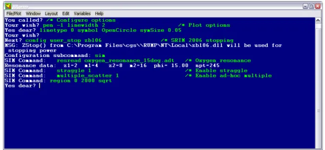
The second step is often to configure some simulation parameters using line commands. In this case, SRIM-2006 stopping powers are used, the non-Rutherford scattering cross section for the 16O(α,α)16O is loaded, and straggling and multiple scattering are enabled. By default, all isotopes are calculated separately (as opposed to making one single calculation for the average mass of the target element), and Andersen electron
The third step is to define the sample structure. This is done using intuitive, easy-to-learn commands. The corresponding first guess is then calculated.
FIG. 14.10. Third step of a RUMP analysis: define the sample structure, perform the simulation.
A manual iterative procedure as described in EXAMPLE 14.1 would follow the first guess. Alternatively, RUMP includes an optimization algorithm. The window shows the definition of the fitting space and the final results. In most situations, not all variables would be fitted at the same time. A combination of manual iterations and fitting of some parameters is typical.