Partial Fiscal Decentralization
by
Jan K. Brueckner Department of Economics University of California, Irvine
3151 Social Science Plaza Irvine, CA 92697 e-mail: [email protected]
September 2007
Abstract
The fiscal decentralization impulse now sweeping the world often leads to partial decentraliza-tion, where subnational governments are funded by central transfers, rather than leading to full local autonomy. Despite the practical important of this arrangement, the literature contains no economic analysis of a partial decentralization regime in a Tiebout-style model. This paper provides such an analysis, relying on the key assumption that public-good provision requires effort on the part of government officials. By choosing different degrees of effort, localities can then provide different public-good levels even when a fixed, common transfer constrains them to spend the same amount. A number of useful results are derived.
Partial Fiscal Decentralization
byJan K. Brueckner*
1. Introduction
Under fiscal decentralization, subnational governments are granted autonomy in the pro-vision and financing of public goods. While subnational autonomy has long been a feature of the fiscal environment in the United States and several other countries, a greater degree of central control over the public sector is common elsewhere, especially in the developing world. However, partly in response to advice from the World Bank and other international agencies, many developing countries are seeking greater fiscal decentralization by attempting to real-locate spending and taxing authority to subnational governments. This movement has been motivated in part by the ideas of Tiebout (1956), who argued that local control of spending allows the public sector to respond more effectively to varied consumer preferences for public goods.
Despite this impulse toward decentralization, an obstacle to the achievement of true local autonomy in developing countries lies on the tax side. Even when spending authority is passed downward to subnational governments, a lack of adequate tax capacity (especially at the local level) often prevents these governments from funding expenditures out of their own revenues. Instead, spending relies heavily on transfers from the central government. As explained by Shah (2004),
. . . decentralization of taxing powers may not fully match the decentralization of ex-penditure and regulatory functions. . . Revenue systems in developing and transition economies are typically characterized by a large and dominant central government role and a heavy reliance on indirect taxes such as VAT, excises, taxes on external trade and fuel taxes. . . Local governments have very limited access to own source revenues such as property taxes and user charges and even for these limited tax bases, they typically have autonomy only with respect to rate setting within limits.
Reflecting limited own source revenues, figures presented by Shah and Shah (2006) show that, in a sample of ten lower-income countries,1 local governments relied on intergovernmental transfers for 51% of their revenue, in contrast to a smaller transfer share of 34% for OECD
countries. For some sample countries (Uganda, Poland, Brazil), the transfer share exceeded 65%. In a larger sample of developing countries analyzed by Shah (2004), 42% of subnational revenue (local and provincial) came from transfers, with the share ranging from 75 to 95% in Indonesia, Nigeria, Mexico, Pakistan and South Africa. Although Shah does not present evidence on tax autonomy for his sample, a separate OECD study (1999) shows that, for one his countries (Mexico), subnational governments had effective control over only 14% of their tax revenue, with all of this control occurring at the state rather than local level. This fact suggests that limits on subnational autonomy may be even tighter than suggested by evidence of a high reliance on transfers.
Despite their reliance on intergovernmental transfers and potentially limited tax autonomy, subnational governments in Shah’s sample had effective control over 58% of their expenditures. Thus, developing countries appear to have more discretion in spending decisions than in the raising of public revenue, which suggests that the usual models from the Tiebout tradition should not be used to analyze their fiscal decentralization experiences. Instead, the appropriate model may be one of “partial fiscal decentralization,” where spending authority is devolved to the subnational level while financing relies on transfers from the central government. The purpose of the present paper is to propose and analyze such a model.
In the model, the central government levies a uniform head tax on each consumer and then transfers the resulting revenue to local governments, which are the only subnational units. The transfers are assumed to occur on a uniform per capita basis, perhaps reflecting a constitutional requirement for equal treatment of all local governments. Since consumer incomes are identical in the model, making regional equalization unnecessary, this uniformity assumption is natural. Under partial decentralization, spending authority resides at the local level. But since local tax revenue is nonexistent by assumption in the basic model, localities must rely entirely on central transfers to finance their expenditures. In a standard setup, this arrangement would allow localities no freedom whatsoever in setting public-good levels, which would be dictated instead by the fixed per capita transfer. However, a key feature of the model gives localities discretion in the provision of public goods. In particular, the public-good cost function depends not only on z, the level of the public good, but also on e, the “effort” level chosen by
local-government officials. Higher effort reduces the per capita cost of providing any given z. Even though this cost is constrained to equal the fixed central transfer, the ability to adjust both z and e means the locality gains discretion in the choice of z even though its spending level is controlled.
Both z and e are chosen taking into account a separate “cost” of effort, which does not appear in the public accounts. Interpreting effort as the education level of government officials, this cost would represent the private cost incurred by these officials in educating themselves, which is not covered by the central transfer.
In characterizing the public-sector equilibrium, the analysis relies on the modern formaliza-tion of the Tiebout model, drawing in particular on the approach of Scotchmer and Wooders (1986).2 Government officials are assumed to collaborate with community developers, who build houses and sell them to consumers. The officials’ objective function equals developer profit, which depends on the attractiveness of the community and hence on the public-good levelz, minus their own cost of effort. This “net profit” objective would be appropriate if the officials themselves played the role of developers, but it also applies in a case in which the officials are separate entities but extract all the developer profit via unmodeled taxes or per-haps bribes. For simplicity, the combined entity composed of developers and their associated government officials is referred to as a “locality” in the analysis.
In the model, Tiebout sorting occurs as localities, using their discretion in the choice of public goods, tailor z to suit consumer preferences, which are assumed to be heterogeneous. In addition, free entry of communities ensures that net profit is zero in equilibrium. The equilibrium public-good levels depend, of course, on the level of the central transfer.
The paper starts by considering two benchmarks against which partial decentralization can be compared. The first is full decentralization, under which localities can use freely-chosen local taxes to finance public goods. The second is full central control, under which the central government specifies a fixed z that each locality must deliver and provides the transfer to finance it (implying a particular required effort level). Note that, despite central control, z must still be delivered locally, reflecting the nature of many public goods.
decentralization is preferred to full central control as long as preferences are heterogeneous. The reason is that full central control needlessly eliminates the variety in z made possible by adjustment of effort levels, which occurs despite the uniformity of the central transfer. Were it feasible, full decentralization would in turn be preferred to partial decentralization since it allows a fuller response to heterogeneous preferences. But with full decentralization ruled out by the lack of local tax capacity, partial decentralization is the preferred fiscal arrangement. This conclusion offers an important practical lesson by showing that, in a setting where local-ities have some discretion in choosing public-good levels despite a fixed spending requirement, the center should relinquish control of this decision, letting localities make their ownzchoices. The analysis then compares patterns of public-good provision under partial and full decen-tralization. The discussion shows that, when the central transfer under partial decentralization is efficiently set at a “compromise” level that lies between the highest and lowest local taxes charged under full decentralization, the dispersion of z levels narrows relative to the full de-centralization case. In other words, relative to full dede-centralization,z rises for low demanders and falls for high demanders under partial decentralization, a natural result. Despite this con-clusion, the dispersion of effort levels could narrow or widen relative to full decentralization depending on the nature of preferences and costs.
Thus, while Tiebout sorting under partial decentralization generates a variety of public-good levels, the variety that emerges is lower than under full decentralization, imposing a cost on society. The analysis also explores how this variety comparison is affected when localities have the ability to levy a modest amount local taxes up to some cap. In this case, public-good variety is only sacrificed at the extremes, with the middle of the z distribution the same as under full decentralization. The foregoing analysis is presented in sections 2 and 3.
The discussion in section 4 then asks whether partial decentralization could sometimes be the preferred institutional arrangement, rather than constituting best response to limitations on local tax capacity. To this end, the model is modified to include a Leviathan motive on the part of local officials, who derive enjoyment from spending tax money beyond any profit earned. Relying partly on numerical examples, it is shown that partial decentralization can be superior to both full central control and full decentralization under this modification. In
such a case, partial decentralization would be the best arrangement even if unlimited local tax capacity made full decentralization feasible. The analysis also briefly considers the effects of other types of undesirable local behavior, including the laziness on the part of government officials, which raises the cost of effort beyond its resource cost, and the theft of tax revenue.
This paper adds to a recent resurgence of research on fiscal decentralization, which builds on the classic treatment of Oates (1972). Recent papers include Lockwood (2002), Besley and Coate (2003), Brueckner (2004) and Lorz and Willman (2005), among others (see Brueckner (2004) for fuller references). In the models of Besley and Coate and Lockwood, the central government is able to provide different z’s across regions when it has the responsibility for public-good provision, an outcome that would be analogous to allowing non-uniform transfers in the present setup. While non-uniformity in these models is the result of a political struggle between regions, non-uniform transfers would only appear to be appropriate in the present model as a means of addressing income equalities, which are absent by assumption.
It is important to recognize that the analysis in this paper is not meant to be a defini-tive treatment of partial fiscal decentralization. Rather, the model is offered as one possible approach to this issue, with the goal of ending the literature’s near-complete silence on the subject. In a rare related study, Schwager (1999) analyzes what he calls “administrative feder-alism,” where the center sets quality standards for public projects executed by localities, and further analysis of incomplete fiscal decentralization from yet other perspectives is needed.
2. Basic Model
As noted above, the per capita cost of public-good provision depends on the level of the good, z, and on the effort of government officials,e. The cost function is writtenC(z, e), with Cz >0 and Ce <0, and the function is assumed to be strictly convex (subscripts denote partial derivatives). Generally, per capita cost should depend on the population n of the community, but this dependence is eliminated via the assumption of constant returns to population, which means that the overall cost function is written nC(z, e).
For future reference, note that C comes from inverting an underlying public-good produc-tion funcproduc-tion, written as z = S(g, e), where g is the physical input and Se > 0. Inverting S
with respect to theg input yieldsg =S−1(z, e), whereS−1 is the appropriate inverse function. With the price of g normalized to unity,C(z, e)≡S−1(z, e).
The cost of effort by government officials, again expressed on per capita basis, is written F(e), where F is a strictly convex, increasing function. This function is again independent of community population, which means that the overall cost of effort isnF(e). This setup follows from assuming that the cost of effort per official is f(e), and that η officials are required per capita, withF(e)≡ηf(e).
Developers build houses of a fixed size, which are rented to consumers. The production cost per house is denotedr, but this cost is normalized to zero for simplicity. The price commanded by a house depends on the community’s public-good level, with this price given by the function P(z), where P >0. This price function is ultimately endogenous but is viewed as parametric by all agents in the economy, following the “price-taking” approach of Scotchmer and Wooders (1986).3
The economy contains m types of consumers, with each having quasi-linear preferences overz and consumption of a private good x. The utility function for type-j consumers is given byx+Uj(z), but for expository convenience, the functions Uj are assumed to take the form θjV(z), where V(·) is strictly concave. The θ parameters satisfy θ1 > θ2 > · · · > θm, so that consumer demand for z weakens as the taste index rises. Consumer incomes are identical and equal toy.
2.1. Full decentralization
Consider now the case of full decentralization, the first of the two benchmark regimes considered in the analysis of partial decentralization. Under full decentralization, localities levy their own taxes to pay for public goods, whose levels are freely chosen. For concreteness, suppose that these taxes are property taxes, paid by the developer of each house. Conditional on z and e, the tax payment per house is then C(z, e), which leaves a profit for the developer equal toP(z)−C(z, e).
is given by
P(z) − C(z, e) − F(e) ≡ π, (1) This expression constitutes the locality’s objective function. As explained above, (1) is appro-priate if government officials are able to capture all the developer’s profit through unmodeled taxes or by soliciting bribes. Alternatively, the government officials themselves could function as developers, so that the profit portion of (1) accrues directly to them.
The locality maximizes (1) by choice of z and e, and the first-order conditions are
P − Cz = 0 (2)
−F − Ce = 0. (3)
The first condition says thatzis optimal when the increment to the house price from a marginal increase equals the marginal cost of z. The effort choice is optimal when the tax reduction
−Ce allowed by higher effort equals the marginal cost of effort. The second-order condition for maximization of (1) is assumed to hold.4
Consumers maximize utility by selecting a community of residence, a choice that reduces to selecting z. A type-i consumer maximizes x+θiV(z) subject to the budget constraint x+P(z) =y, and the first-order condition is
θiV = P . (4)
From the consumer’s point of view,z is optimal when marginal utility equals the incremental rent from a marginally higherz.
To understand the model’s equilibrium, suppose for a moment that all consumers are of type i. Then, each consumer demands the z level given by solution to (4), while localities provide thez level given by the solution to (2)–(3). In equilibrium, thesez values must be the same, so that localities provide the public-good level demanded by consumers.
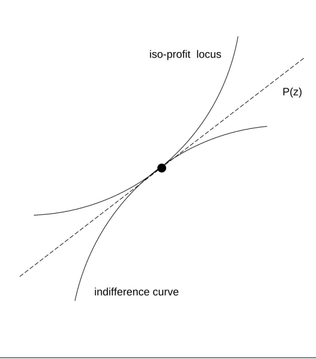
This equivalence is ensured by the shape of the equilibrium price function, as illustrated in Figure 1. To understand this claim, observe that consumer maximization requires tangency between an indifference curve in (P, z) space and price function P(z), while net profit maxi-mization by localities requires a tangency between an iso-profit locus and the price function.5 For equilibrium to obtain, these tangencies must occur at the same point, as seen in Figure 1. An equilibrium price function must have the proper shape to ensure this coincidence of tangencies. WhileP(z) is shown as linear for simplicity, the function can take other forms.6
Coincident tangencies mean, of course that the indifference curve and iso-profit locus must be tangent to each other at the equilibrium point, which requires θiV = Cz. Formally, this condition comes from the requirement that (2) and (4) hold at the same value of z, which allows the equations to be combined, eliminatingP . Together, this tangency condition along with (3) determine the equilibrium values ofz and e, denoted zi∗ and e∗i:
θiV(zi∗) = Cz(z∗i, e∗i) (5) F(e∗i) = −Ce(zi∗, e∗i). (6)
A further equilibrium requirement, which comes from the assumption of free entry by localities, is that net profit equals zero. This requirement effectively pins down the level of the equilibrium price function, with its slope constrained by the double-tangency requirement. With zero net profit requiringP(z) =C(z, e) +F(e), private good consumption is then given byx∗i =y−P(zi∗) =y−C(z∗i, e∗i)−F(e∗i), completing the determination of all the variables in the model.
When multiple consumer types exist, each type maximizes conditional on P(z), yielding a collection of different demandedzlevels. All these levels must be provided by different localities in equilibrium, which requires a set of coincident indifference-curve/iso-profit tangencies along the price function. Since zero profit is required in equilibrium, all these tangencies must then lie on the zero-profit locus. To generate this outcome, the equilibrium price function must “thread” all the tangency points, passing through each one in the manner seen in Figure 1.7
The key feature of this equilibrium is Tiebout sorting, with the various taste groups con-suming different public-good levels,zj∗, j = 1, . . . , M, in separate localities. These levels are in turn provided using different degrees of effort,e∗j,j = 1, . . . , M, with all the solutions given by the analog to (5)–(6) for the various taste groups. For future reference, let the resulting public-good costs be denoted Tj∗ = C(zj∗, e∗j). Since public-good demand falls with index of the consumer, it follows thatT1∗ > T2∗>· · ·> Tm∗.8
2.2. Full central control
The other benchmark regime, full central control, leaves localities no discretion in choosing public-good and effort levels. Under this arrangement, the central government collects a head tax T from each consumer, and then transfers this tax revenue to localities on an equal per capita basis. In addition, the center mandates a common public-good level z, which each community is required to provide (z must feasible given the available transfer). This mandate then determines a required effort levele, which satisfies T =C(z,e).
Under full central control, local taxes are absent, so that developer profit is P(z) and the net profit of each locality is P(z)−F(e). Free entry again must reduce net profit to zero, so that P(z)−F(e) = 0 holds and x = y−T −F(e). The outcome under full central control depends on the chosen values ofT and z, which are considered below.
2.3. Partial decentralization
The discussion now turns to the main focus of the analysis, the case of partial decentral-ization. Under this regime, the center collects a head tax ofT, which is transferred to localities on an equal per capita basis. However, in contrast to full central control, the center does not mandate a particular public-good level, but instead leaves the choice of z up to the localities. Local taxes are again absent, so that a locality’s net profit equals P(z)−F(e). Net profit is now maximized subject to the constraint thatT exceeds or equals the public-good cost. Given that effort is costly, this constraint will bind in equilibrium, and it is written
T = C(z, e). (7)
localities discretion in the choice of public goods despite central control of their spending. Letting λ denote the multiplier associated with the constraint, the Lagrangian expression for maximization of net profit is P(z)−F(e) +λ(T −C(z, e)), and the first-order conditions are9
P − λCz = 0 (8)
−F − λCe = 0. (9)
In the case of a single consumer type, again denoted i, localities must provide the z level demanded by that type. This equilibrium requirement again allows the P term in (8) to be replaced by θiV, yielding θiV = λCz. Thus, the equilibrium solutions for the partial decentralization regime, denotedzi,ei, and λi, satisfy
θiV(zi) = λiCz(zi,ei) (10) F (ei) = −λiCe(zi,ei) (11)
T = C(zi,ei). (12)
In addition, the zero-profit condition again yieldsxi=y−P(zi) =y−C(zi,ei)−F(ei). Note that all of the solutions are conditional on T.
When multiple consumer types exist, equilibrium conditions analogous to (10)–(12) emerge for each type. Thus, as in the case of full decentralization, the equilibrium is characterized by Tiebout sorting, with the various types consuming different public-good levels in separate localities. This outcome emerges even though each locality is required to spend the same amount, a consequence of the flexibility made possible by variable effort.
A key task is to compare the public-good levels chosen under full and partial decentraliza-tion. This task is undertaken below, following an efficiency comparison of the three different regimes.
3. Comparing Partial to Full Decentralization and Full Central Control
3.1. Efficiency comparisonsIn comparing partial decentralization to the two benchmark regimes, it is useful to first make an efficiency comparison. The verdict is immediate given that progression from full central control to partial decentralization to full decentralization involves successive relaxation of constraints, implying increases in potential welfare. This point is demonstrated in the ensuing discussion.
Welfare in the model equals total consumer utility plus the total net profit of localities. Since profit is zero, welfare is simply total utility, written taking the zero-profit constraint into account. Letting ρj be the type-j population share, j = 1, . . . , m, per capita welfare is then equal to W = m j=1 ρj[y − Tj − F(ej) + θiV(zj)], (13) where Tj = C(zj, ej), i= 1,2, . . . , M. (14) Under unrestricted welfare maximization, W is maximized treating zi, ei and Ti, i = 1, . . . , M, as choice variables, with the conditions in (14) treated as constraints. The first-order conditions are ρiθiV(zi) = µiCz, ρiF = −µiCe, and µi = ρi. Since these conditions reduce to the equilibrium conditions (5) and (6) under the full decentralization regime, full decentralization is welfare maximizing, reflecting the usual Tiebout result for the present model.
By contrast, partial decentralization is captured by adding the constraints
Tj = T , j = 1,2, . . . , M, (15) to the maximization problem in (13)–(14). It is again easily seen that the optimality conditions forzi and ei in this restricted problem reduce to the equilibrium conditions (10) and (11) (see the appendix). This equivalence shows that the partial decentralization equilibrium is efficient conditional onT. Choosing the value ofT optimally then yields the best possible outcome for this regime, and the relevant first-order condition is discussed below.
Finally, the regime with full central control is captured by replacing T by T in (15) and adding the further constraints
zj = z, j = 1,2, . . . , M (16)
to the maximization problem (13)–(15). T andz can then be chosen optimally.
Since the progression between the above problems involves the successive addition of con-straints, which reduce the maximal value of the objective function, the following conclusion can be stated:
Proposition 1. If T is chosen optimally, then welfare rises moving from full central control to partial decentralization to full decentralization.
It is easily seen that, if the taste groups are identical, then this result is overturned, with the same welfare achieved under the three different regimes. Observe also that, ifT is not chosen optimally, then the welfare comparison between full central control and partial decentralization could be reversed.10
Proposition 1 implies that, if full decentralization is feasible under a country’s institutional structure, it is the preferred regime. However, if limitations on local tax capacity require revenue to be raised by the central government and then transferred to localities, these transfers should occur under a regime of partial decentralization, where local spending autonomy is permitted. The alternative of full central control, where the center provides transfers and mandates public-good levels, is inferior to partial decentralization as long as the center can identify the optimal T or come close to it. Full central control needlessly restricts variety in the provision of public goods, which emerges through adjustment of effort levels under partial decentralization despite the fixed spending requirement.
3.2. The optimal T
Further comparisons require a characterization of the optimal transfer level under partial decentralization, which is derived by collapsing the welfare-maximization problem for that regime into a simpler form. To do so, T replaces Tj in (13) and (14), with the constraints in
(15) dropped, yielding the Lagrangian expression m j=1 ρj[y − T − F(ej) + θiV(zj)] + m j=1 µj[T − C(zj, ej)] (17)
From (17), the first-order condition for T is m i=1 µj = m i=1 ρj = 1, (18)
which can be rewritten as mj=1ρjθjV(zj)/Cz(zj, ej) = 1 using the first-order condition for zj to eliminate µj (see the appendix). In this form, the optimality condition says that the weighted average across consumer types of the ratio ofz’s marginal utility to its marginal cost must equal unity. The optimality conditions for full central control have a related form.11
Condition (18), though not intuitive, is useful in characterizing the magnitude of the optimal T, denoted T∗. Recalling that Ti∗ = C(zi∗, e∗i) gives the public-good cost under full decentralization, the following result (proved in the appendix) is useful:
Lemma 1. The multiplier µi satisfies µi >(=) < ρi as T < (=)> Ti∗, i= 1, . . . , m.
For (18) to hold, the multiplierµimust be larger than the population shareρifor someivalues and smaller for others, and the lemma shows that the pattern depends on the relationship between the Ti∗ and T. Since satisfaction of the inequality µi ≥ ρi for all i is ruled out, as is satisfaction of µi ≤ρi, the lemma then implies that T ≤Ti∗ or T ≥ Ti∗ cannot hold for all i, yielding
Proposition 2. T∗ must satisfy T1∗ >T∗ > Tm∗.
Recalling that T1∗ and Tm∗ are the largest and smallest Ti∗’s under full decentralization, the proposition says that the optimal T is bracketed by these minimal and maximal values, a natural result.
Although the optimal T has been characterized, central governments do not possess the information on preferences and costs required to compute such a value. Localities, by contrast, in maximizing net profit in response to an equilibrium price function for housing, make optimal choices even though they also lack information about consumer preferences. Nevertheless, despite their lack of information, central governments might setT in an approximately optimal fashion. Indeed, it might be reasonable to suppose that the center would be able to select T with the same precision reflected in Proposition 2, settingT somewhere between the maximal and minimal Ti∗ values under full decentralization. This kind of selection is referred to as a “compromise choice” of T.
Assuming that the center makes a compromise choice, the analysis next investigates the distribution ofz values under partial decentralization.
3.3. Comparing the distribution of z values under full and partial decentralization
With a compromise choice of T, public-good costs rise for some consumer types and fall for others, relative to the full decentralization regime. Finding the effect on public-good levels requires assessing the impact ofT on z, recognizing thatTi∗under full decentralization can be treated as a particular value of T.
To carry out this exercise, the equilibrium conditions (10) and (11) under partial decen-tralization can be collapsed into the single condition
θiV(zi)
F (ei) = −
Cz(zi,ei)
Ce(zi,ei). (19) This condition, along with (12), determines zi and ei conditional on T. Equivalently, the equilibrium conditions (5) and (6) under full decentralization can be collapsed into an equation analogous to (19), with the hats replaced by asterisks. Since the equality Ti∗ = C(zi∗, e∗i) is analogous to (12), the full decentralization equilibrium values for locality i can be generated under partial decentralization by settingT equal toTi∗. As a result, the impact of T onzican be used to compare thez values emerging under the two regimes.
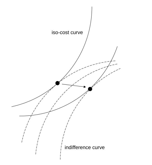
Although comparative-static analysis ofT’s effect is messy, insight is gained by considering a diagram, as follows. The RHS of (19) is the slope of an iso-cost curve in (z, e) space, defined
by (12) and shown in Figure 2. Since a higherT allowse to be reduced while holding z fixed, the locus shifts downward as T increases. In addition, strict convexity of C implies that the function is also strictly quasi-convex, so that the locus has the convex curvature shown in the Figure.
The LHS of (19) is the slope of an indifference curve in (e, z) space, as defined by y−
T −F(e) +θiV(z) = u and shown in Figure 2. Note that the indifference curve is concave because, as z and e increase moving along the curve, the numerator of the slope expression falls while the denominator rises. Note also that slope at a given (e, z) point is independent of the magnitude ofT. Thus, (19) characterizes a tangency between an iso-cost curve and an indifference curve, as seen in the Figure.
When T increases, the iso-cost curve shifts down, and a new tangency point is established. The resulting direction of change for z depends on the changes in the slopes of the two curves moving vertically downward from the original tangency. First, note that, since F > 0, a decline in e with z held fixed raises the indifference-curve slope. However, the change in the slope of the iso-cost curve is ambiguous, making the change in z ambiguous in general. But if the physical input g into public good production is normal, in the sense that its cost-minimizing level rises as the target amount ofz output increases, then the iso-cost curve slope flattens moving vertically downward (see the appendix for a proof). With the indifference curve steepening, and the curves respectively convex and concave, the tangency must then move to the right, as shown in Figure 2. Thus, an increase in T raiseszi. However, as should be clear from the Figure, nothing general can be said about the direction of the change forei. This discussion establishes
Lemma 2. If the physical input into public-good production is normal, then an increase in T raiseszj for all j.
The normality property in the lemma will henceforth be a maintained assumption.
For a type-i consumer, moving from the full decentralization regime to partial decentral-ization can be viewed as a change inT from a value of Ti∗to the whatever value prevails under the latter regime. A compromise choice, which setsT at a value T#, can then be viewed as an
increase inT for consumer types withTi∗<T#, whose z values under full decentralization are low, and a decrease inT for types with Ti∗ >T#, whose z values are high. From the lemma, these changes in turn yield increases and decreases, respectively, in z. Thus,
Proposition 3. A compromise choice of T under partial decentralization narrows the dispersion of z levels relative to full decentralization case.
This result, which is a natural conclusion, shows that the consequences of Tiebout sorting are muted under partial decentralization. Since public-good costs are constrained to be equal across localities, partial decentralization reduces the variety in available z levels. However, some variety is still available, a key conclusion that makes partial decentralization superior to full central control.
Although the effect of partial decentralization on the dispersion of effort levels is ambiguous in general, a clear impact emerges under specific functional forms. In particular, if the z production function is Cobb-Douglas, withz =g1/αeβ/α (yieldingC(z, e) =zαe−β), ifV(z) = zδ, and ifF(e) =eγ, then the solution to (19) and (12) shows that bothziandeiare increasing inT. As a result, following the above logic, partial decentralization narrows the dispersion of both z and e levels relative to the full decentralization regime.
3.4. The effect of allowing limited local tax capacity
Suppose realistically that, instead of relying entirely on central transfers, localities have limited taxing ability, being allowed to a levy local (property) tax t up to a per capita limit of t. In this case, a locality’s net profit is P(z) −t −F(e), which is maximized subject to the constraints t ≥ 0, t ≥ t, and T + t = C(z, e). The Lagrangian expression is thus P(z)−t−F(e) +λ(T+t−C(z, e)) +νt+τ(t−t). The first-order conditions forz and eare again (8) and (9), and thet condition is
−1 + λ + ν − τ = 0. (20)
If the constraints on t are not binding, then ν = τ = 0 and hence λ = 1. Eqs. (8) and (9) then reduce to the first-order conditions (2) and (3) for the full decentralization case,
ultimately yielding the equilibrium conditions (5) and (6) for any consumer type where the constraints on the local tax are not binding. This conclusion is natural: free adjustment of local taxes on top of a fixed transfer allows public spending to be freely chosen, just as in the full decentralization case. However, if one of the constraints on t binds, the outcome for that consumer type mirrors the original partial decentralization regime.
With a sufficient range of demands for z in the population, a small enough cap t, and a compromise choice ofT, the nonnegativity constraint ontwill bind for the lowest public-good demanders and the upper cap will bind for highest demanders. For moderate demanders, choice of t will be unconstrained. Applying the logic of section 2.3 then yields
Proposition 4. Under partial decentralization with local taxes, supposeT is set so that the constraint t ≥0 binds for at least one low-z-demand consumer and the constraint t ≥ t binds for at least one high-demand consumer. Chosen z levels are then higher (lower) than under full centralization for these constrained low (high) demanders, with the z distribution compressed at the top and bottom. For unconstrained individuals, chosen z’s match those under full decentralization.
It is also interesting to consider the efficient choice ofT in the presence of local taxes. The Lagrangian for the welfare maximization problem is
ρj[y−F(ej)−T−tj−θjV(zj)] + µj[T+tj−C(zj, ej)] + νjtj +τj(t−tj) (21)
As before, the first-order conditions for zi and ei under partial decentralization match the equilibrium conditions, while the conditions fortiand T are −ρi+µi+νi−τi = 0 andµj =
ρj. When neither t constraint is binding,µi=ρi holds, so that the T condition reduces to
j∈Aµj = j∈Aρj, where A is the set of constrained consumers. Recognizing that the set A contains those individuals with the maximal and minimal values of Ti∗ and repeating the previous logic, it follows that Proposition 2 continues to hold. Moreover, using the first-order condition forzito eliminateµi, theTcondition can be written asj∈AρjθjV(zj)/Cz(zj, ej) =
j∈Aρj, indicating that only the preferences of individuals in the constrained group matter in the determination of T. The preferences of the unconstrained demanders in the middle of the distribution, who have effective local control over public spending, are not considered.12
4. Adding Local Leviathan Behavior
4.1. Basic analysisIn analysis so far, full decentralization is always preferred, although it may not be feasible due to limitations on local tax capacity. In this case, the partial decentralization regime is the best available option. This section of the paper modifies the model in a way that reduces the attractiveness of full decentralization, possibly making partial decentralization the preferred arrangement even in the absence of any limits on local tax capacity. The modification consists of Leviathan behavior on the part of local officials, which is captured by assuming that the officials receive a utility equal toφC(z, e) from spending on public goods, over and above the locality’s net profit.
In the case of full decentralization, net locality profit plus Leviathan utility equals P(z)− C(z, e)−F(e) +φC(z, e). In this case, the Cz and Ce terms in (2) and (3), the first-order conditions for the locality’s maximization problem, are multiplied by the factor 1−φ, and previous type-i equilibrium conditions, (5) and (6), are replaced by
θiV(zi∗∗) = (1−φ)Cz(zi∗∗, e∗∗i ) (22) F(e∗∗i ) = −(1−φ)Ce(zi∗∗, e∗∗i ), (23)
where the double asterisks indicate equilibrium values with Leviathan behavior. Note that such behavior reduces the perceived marginal cost of z as well as the perceived cost savings from higher effort. Let
T∗∗
i = C(zi∗∗, e∗∗i ) (24) denote the public-good cost under full decentralization.
To evaluate the efficiency of this equilibrium, consider the welfare maximization problem. The utility for a type-iconsumer isy−P(zi)−Ti+θiV(zi), and net profit plus Leviathan utility fori’s locality equalsP(zi)−F(ei) +φTi. While summing yieldsy−Ti−F(ei) +θiV(zi) +φTi, the social planner does not treat Leviathan utility as a social return and thus subtracts it in reaching a final welfare measure for localityi, which then equalsW =y−Ti−F(ei) +θiV(zi),
withTi =C(zi, ei). Multiplying byρiand summing acrossi, the welfare maximization problem is thus identical to the problem given by (13) and (14).
Given this fact, Lemma 1 can be used to compare Ti∗∗from (24) to the socially optimalTi, which equals the efficient equilibrium valueTi∗ in the basic model. The following result can be established (see the appendix):
Proposition 5. Tj∗∗ > Tj∗ holds for all j, so that public-good cost for each consumer type under full decentralization exceeds the socially optimal level. As a result, zj∗∗ > z∗j also holds for all j, so that public goods are overprovided.
These results are, of course, natural ones given Leviathan behavior.
Turning to the partial decentralization regime under Leviathan behavior, a locality’s La-grangian expression is given by P(z)−F(e) +φT +λ(T − C(z, e)). It is easily seen that the resulting first-order and equilibrium conditions are unchanged, being given by (8)–(9) and (10)–(12) respectively. Leviathan behavior thus has no effect on the equilibriumz andevalues under partial decentralization, conditional on T. Moreover, given that the welfare maximiza-tion problem is unchanged, it remains true that the partial decentralizamaximiza-tion equilibrium is efficient conditional on T. The magnitude of T∗, the optimal value of T, is also unchanged.
Given these facts, Proposition 2 continues to hold. But since the efficient Ti∗ values in the proposition are no longer equilibrium values under full decentralization, the comparison of T∗ to the equilibrium values (Ti∗∗, i = 1,2, , . . . , m) is disrupted. Using Proposition 5, the following more-limited result emerges:
Proposition 6. T∗ satisfies T1∗∗ >T∗, but T∗ can be larger or smaller than Tm∗∗.
Thus T∗ is no longer bracketed by the largest and smallest equilibriumTi values under full decentralization. Since the distribution of these values shifts to the right, the smallest value may no longer be smaller than T∗.
If the center’s choice of T under partial decentralization is approximately optimal, so that it falls short of T1∗∗, then z values will be lower than under full decentralization for the highest-demand consumers (those with Tj∗∗ > T). If T > T m∗∗ holds in addition, then
partial decentralization will raise z values for the lowest-demand consumers, preserving the compression property of the basic model, as stated in Proposition 3. However, if T < T m∗∗ holds, then partial decentralization will reduce thez’s of all consumers.
4.2. Welfare comparisons
While full decentralization was unambiguously superior to partial decentralization in the basic model, a different conclusion emerges under Leviathan behavior. To explore this question, it is useful to start by considering a model with a single consumer type, denoted i. In this case, W =y−Ti−F(ei) +θiV(zi). Maximizing with respect to all three variables subject to Ti=C(zi, ei), the conditionsθiV=Cz andF =−Ce characterize the social optimum. These conditions are satisfied under partial decentralization whenT is set equal to Ti∗ and (trivially) satisfied under full central control when T =Ti∗ and zi=z∗i. Thus, with one consumer type, these two regimes are equivalent and both can generate the full social optimum. By contrast, welfare under full decentralization is lower, a consequence of the Leviathan distortion.
Although full decentralization is inferior with a single consumer type, consumer hetero-geneity complicates the welfare comparison. In this case, movement from full central control to partial decentralization is welfare improving because control overT can still restrain Leviathan behavior, while localities gain discretion over z. Further movement to full decentralization, however, has both positive and negative effects: localities gain even more discretion to respond to consumer public-good demands, but their Leviathan tendencies are unrestrained. These considerations indicate that partial decentralization may be superior to full decentralization in some situations and not in others. Intuition would suggest that, if the strength of Leviathan motive (as measured by the size ofφ) is large relative to the dispersion of z demands, then the negative effect of moving to full decentralization would dominate the positive effect, making partial decentralization preferable. The outcome would be reversed, making full decentral-ization preferable, when demand dispersion is high relative to the strength of the Leviathan motive.
To evaluate these predictions, numerical examples are computed using the functional-form assumptions at the end of section 3. Parameter values are α = 1.5, β = 0.4, δ = 0.75, γ = 1, and φ = 0.25. The population has two equal-size groups, whose θ values are varied in
generating the examples. Table 1 shows welfare levels andT, z, andevalues for three different combinations of the demand parameters (θ1, θ2), which reflect increasing demand dispersion: (4.5, 3.5), (5,3), and (6,2). Note that since the meanθ always equals 4, the solution under full central control is the same in each case.
In the first panel of Table 1, where demand dispersion is low, partial decentralization is the preferred regime. Its welfare level (103.30) exceeds welfare under both full central control (103.28) and full decentralization (102.50). Note that while T1∗∗ (17.45) exceeds T (5.51), following Proposition 6, T2∗∗ (7.55) is also larger than T. As a result, both z1 and z2 are lower under partial than under full decentralization, a comparison that also applies to effort levels. The second panel, where demand dispersion is somewhat higher, shows the same welfare comparison between the regimes. However,T (5.61) is now greater than T2∗∗ (4.52), with the result that thez and e distributions under partial decentralization are compressed relative to full centralization, as in the basic model.
In the third panel of Table 1, demand dispersion is yet greater, but now the welfare ranking of the regimes differs, with full decentralization (W = 104.67) preferred to partial decentralization (W = 103.65). The T, z and e comparisons, however, follow the pattern of the second panel. The welfare reversal seen in these results matches the predictions of intuition, yielding
Proposition 7. With Leviathan behavior, partial decentralization may be preferred to both full central control and full decentralization. This outcome may obtain when public-good demand dispersion is low relative to the strength of the Leviathan motive.
2.3. Other undesirable behavior by localities
Other types of undesirable behavior on the part of localities can be envisioned. For example, local government officials could steal a portion of tax or transfer revenue, with the proceeds adding to their utility. However, it is easily seen that this behavior is self-defeating. The reason is that the theft reduces public-good output, which in turn lowers developer profits by depressing house prices. Thus, since the gain from theft is exactly offset by in a drop in profit, officials have no incentive practice it.
Laziness on the part of officials might be another distortion. This behavior could be modeled by appending a coefficientξ >1 to the effort cost functionF. The extra cost (ξ−1)F could represent a subjective dislike of effort on the part of officials that is not recognized as a social cost by the planner. In contrast to Leviathan behavior, laziness distorts outcomes under both partial and full decentralization, making full central control potentially the preferred regime. Numerical results confirm this prediction when demand dispersion is low or ξ large, but they also show that partial decentralization is now worse than both the other regimes, an apparent consequence of its inability to curb laziness and its allowance for only limited discretion in public-good provision.
5. Conclusion
The fiscal decentralization impulse now sweeping the world often leads to partial decentral-ization, where subnational governments are funded by central transfers, rather than leading to full local autonomy. When it occurs, the choice of partial fiscal decentralization is often dictated by a lack of subnational tax capacity. Despite the practical important of this ar-rangement, the existing literature contains no economic analysis of a partial decentralization regime. This paper has provided such an analysis, relying on the key assumption that public-good provision requires effort on the part of government officials. By choosing different degrees of effort, localities can provide different public-good levels even when a fixed, common transfer constrains them to spend the same amount.
The paper shows that, as long as the transfer under partial decentralization can be chosen in a close-to-optimal fashion, that regime is superior to full central control, where the center dictates common public-good levels along with a fixed amount of spending. This conclusion provides a key practical lesson: when localities are able to adjust public-good levels despite a fixed spending requirement, the center should relinquish control of this decision, allowing localities to make their ownz choices.
The analysis also shows that public-good variety is lower under partial decentralization than under the preferred but infeasible full decentralization regime, muting the consequences of Tiebout sorting. However, if localities can complement the fixed central transfer with limited
local tax revenue, constrained by a cap, then public-good variety is constrained only for high and low demanders, with the center of the distribution unaffected relative to full decentraliza-tion. Finally, Leviathan behavior on the part of local officials leads to overspending under full decentralization, so that partial decentralization may become the preferred arrangement even when full decentralization is institutionally feasible.
Given the practical importance of partial decentralization in the world-wide movement to fiscal decentralization, the kind of analysis presented in this paper offers a needed complement to the existing Tiebout literature. However, as mentioned in the introduction, the present approach offers only one possible perspective on partial decentralization. Further development of realistic models designed to give insight into this important fiscal arrangement deserves high priority.
Appendix
Proof of Lemma 1.
The (zi, ei) choice in maximization of (17) can be treated as a separate problem for each consumer typei. Accordingly, the first-order conditions for the type-iproblem are
ρiθiV(zi) − µiCz(zi, ei) = 0 (a1)
−ρiF(ei) − µiCe(zi, ei) = 0 (a2)
T − C(zi, ei) = 0. (a3) Note that (a1) and (a2) are equivalent to the equilibrium conditions under partial decen-tralization, with the multipliers related by a proportionality factor. This fact establishes the efficiency of the partial decentralization equilibrium, conditional onT. As noted in section 3.1, µi =ρi must hold when T =Ti∗, in which case (a1) and (a2) reduce to the type-i optimality conditions under full decentralization, given by (5) and (6).
Using (a1)–(a3), the second-order condition for the type-i problem requires positivity of a bordered-Hessian determinant: H ≡ det ⎛ ⎜ ⎝ ρiθiV−µiCzz −µiCze −Cz −µiCze −(ρi+µiCee) −Ce −Cz −Ce 0 ⎞ ⎟ ⎠ > 0. (a4)
The next step is to derive the impact of an increase in T on the value of the multiplierµi. Totally differentiating the first-order conditions and using Cramer’s rule yields
∂µi ∂T = 1 H det ⎛ ⎜ ⎝ ρiθiV−µiCzz −µiCze 0 −µiCze −(ρi+µiCee) 0 −Cz −Ce −1 ⎞ ⎟ ⎠ (a5)
From above, the value of ∂µi/∂T when T =Ti∗ is found by evaluating (a5) with µi =ρi. The result is
given the maintained assumptions on the functions C, F and V. With both µi = ρi and ∂µi/∂T < 0 holding whenT =Ti∗, it follows thatµi>(=)< ρiasT < (=) > Ti∗, establishing the lemma.
Proof of Lemma 2.
The lemma is established by showing that the iso-cost slope flattens moving downward in Figure 2. Totally differentiating the production functionz =S(g, e) yields
∂g ∂z = 1 Sg ≡ Cz (a6) ∂g ∂e = − Se Sg ≡ Ce (a7)
Hence, the iso-cost slope can be written
−CCz e = 1 Se(g, e) = 1 Se(C(z, e), e). (a8) Differentiating (a8) with respect to e then yields
−∂e∂ C z Ce = −See+SegCe S2 e = − See−SegSe/Sg S2 e . (a9)
If g is a normal input, then the absolute z-isoquant slope in (g, e) space, given by Sg/Se, increases moving vertically (toward higherevalues), requiringSee−SegSe/Sg <0.13 Eq. (a9) then implies that iso-cost slope rises as e increases holding z fixed, establishing the desired result.
Positivity of (a9) also implies that Ti∗ rises with θi, as asserted earlier. This conclusion comes from total differentiation of (5)–(6) to compute∂Ti∗/∂θi=Cz(∂zi∗/∂θi) +Ce(∂e∗i/∂θi). The resulting expression has the same sign asCzF +CzCee−CeCze, and while the first term is positive, the difference between the last two terms is also positive given positivity of (a9).
Proof of Proposition 5.
The equilibrium system (22)–(24) is equivalent to the system (a1)–(a3) with µi < ρi and
T = Ti∗∗. Therefore using Lemma 1, it follows that Ti∗∗ > Ti∗. While (19) was used above to compare z levels in the full and partial decentralization regimes, the equation can also be used to compare z’s in the full decentralization cases with and without Leviathan behavior, given thatφcancels in combining (22) and (23). This fact means that thez difference between the two cases is determined entirely by the different inTi values. Using Lemma 2 along with T∗∗
indifference curve
iso-profit locus
z
P
Figure 1: The equilibrium
P(z)
function
indifference curve
iso-cost curve
z
e
Table 1
Numerical Examples
full partial full
decentralization decentralization central control θ1 = 4.5 θ2 = 3.5 W 102.50 103.30 103.28 T∗∗ 1 17.45 – – T∗∗ 2 7.55 – – T∗ or T∗ – 5.51 5.47 z1 10.46 4.00 3.83 z2 4.79 3.68 3.83 e1 5.24 2.55 2.19 e2 2.26 1.86 2.19 θ1 = 5 θ2 = 3 W 102.93 103.37 103.28 T1∗∗ 24.79 – – T2∗∗ 4.52 – – T∗ or T∗ – 5.62 5.47 z1 14.52 4.21 3.83 z2 2.96 3.55 3.83 e1 7.44 2.94 2.19 e2 1.36 1.55 2.19 θ1 = 6 θ2 = 2 W 104.67 103.65 103.28 T∗∗ 1 45.53 – – T∗∗ 2 1.17 – – T∗ or T∗ – 6.08 5.47 z1 25.60 4.78 3.83 z2 0.84 3.32 3.83 e1 13.66 3.88 2.19 e2 0.35 0.98 2.19
References
Berglas, E., 1976. On the theory of clubs. American Economic Review 66, 116-121.
Berglas, E., Pines, D., 1980. Clubs as a case of competitive industry with goods of variable
quality. Economics Letters 5, 363-366.
Besley, T., Coate, S., 2003. Centralized vs. decentralized provision of local public goods:
A political economy analysis. Journal of Public Economics 87, 2611-2637.
Brueckner, J.K., 2000. A Tiebout/tax-competition model. Journal of Public Economics
77, 285-306.
Brueckner, J.K., 2004. Fiscal decentralization with distortionary taxation: Tiebout vs. tax
competition. International Tax and Public Finance 11, 133-53.
Lockwood, B., 2002. Distributive politics and the costs of centralization. Review of
Eco-nomic Studies 69, 313-337.
Oates, W.E., 1972. Fiscal Federalism. Harcourt Brace, New York.
OECD, 1999. Taxing Powers of State and Local Governments. Organization for Economic
Cooperation and Development, Paris.
Scotchmer, S., Wooders, M., 1986. Competitive equilibrium and the core in club
economies with nonanonymous crowding. Journal of Public Economics 34, 159-173.
Tiebout, C.M., 1956. A pure theory of local expenditures. Journal of Political Economy64,
416-424.
Schwager, R., 1999. Administrative federalism and a central government with regionally
based preferences,International Tax and Public Finance 6, 165-189.
Shah, A., 2004. Fiscal decentralization in developing and transition economies, unpublished
paper, World Bank.
Shah, A., Shah, S., 2006. The new vision of local governance and the evolving roles of local
Footnotes
∗I thank Kangoh Lee for helpful discussions. Any shortcomings in the paper, however, are my responsibility.
1The countries are Argentina, Brazil, Chile, China, India, Indonesia, Kazakhstan, Poland, South Africa, and Uganda.
2See also Berglas and Pines (1980).
3The alternate “utility-taking” approach to analysis of local public-good provision is exem-plified by Berglas (1976).
4This condition requires positivity of Hessian determinant of (1), or−(P −Czz)(Cee+F )− Cze2 > 0.
5The indifference curve with utilityuis defined by y−P+θiV(z) =u, orP =y−u+θiV(z), an increasing and strictly concave function in (P, z) space. An iso-profit locus is defined by max{e}[P −C(z, e)−F(e)] =π. Using the envelope theorem,∂P/∂z =Cz, and ∂2P/∂z2 = Czz+Cze(∂e/∂z) =CzzCee−Cze2 +CzzF >0.
6The equilibrium price function is not unique. Any function that “threads” the tangency point between an indifference curve and zero-profit locus is an equilibrium function.
7See Brueckner (2000) for a diagram of this type based on a somewhat different model. 8These relationships hold under a weak assumption introduced below.
9The second-order conditions, which now involve a bordered Hessian determinant, are as-sumed to hold.
10Note that optimal choice ofT and z is not required in Proposition 1. ProvidedT is optimal, full central control is inferior to partial decentralization when these variables are chosen optimally, and the outcome is even worse otherwise.
11The optimality conditions for the uniform z and e levels under full central control are
ρ
e∗, and T∗≡C(z∗,e∗).
12It should be recognized that the makeup of the constrained groups itself depends on the magnitude of T, a subtlety that is implicit in the above discussion.
13The cost-minimizinggthen increases as the target level ofzoutput rises, assuming a constant “price” per unit of effort.