IMORC: An Infrastructure and Architecture Template for Implementing
High-Performance Reconfigurable FPGA Accelerators
Tobias Schumacher, Christian Plessl, Marco Platzner
Paderborn Center for Parallel Computing, University of Paderborn, 33098 Paderborn, Germany
Abstract
The design, implementation and optimization of FPGA accelerators is a challenging task, especially when the accelerator comprises multiple compute cores distributed across CPU and FPGA resources and memories and exhibits data-dependent runtime behavior. In order to simplify the development of FPGA accelerators we propose IMORC, an infrastructure and architecture template that helps raising the level of abstraction. The IMORC development flow bases on a modeling technique for visualizing an application’s communication demand and an architecture template that aids the developer in implementing the design. The architectural template consists of a versatile on-chip interconnect with asynchronous FIFOs and bitwidth conversion placed into the communication links, a performance monitoring infrastructure for collecting performance information during runtime and a set of generic infrastructure cores which are frequently needed in accelerator designs. We demonstrate the usefulness of the IMORC development flow by means of the case study of accelerating thek-th nearest neighbor thinning problem, where IMORC greatly helps us in understanding the communication demand and in implementing the application. With the integrated performance monitoring infrastructure, we gain insights into the data-dependent behavior of the accelerator that helps us in identifying bottlenecks and optimizing the accelerator to achieve a speedup of 10×-40×over an optimized CPU implementation.
Keywords: reconfigurable computing, k-th nearest neighbor technique, FPGA
1. Introduction
While research has demonstrated the potential of FPGAs as acceleration technology since decades, the creation of accel-erators for realistic workloads has been hindered, at least par-tially, by the lack of commercially available systems. In the last years, however, computing system vendors began to offer machines that combine microprocessors with FPGAs. More re-cently, FPGA modules that fit into processor sockets have been introduced, e.g., [1, 2], and provide a fairly standardized way of integrating hardware accelerators into mainstream comput-ing systems.
Developing and optimizing accelerators for such machines is a challenge. Even if FPGA cores for important algorith-mic kernels become more and more available, combining them into an overall accelerator remains tricky. Generally, the cores will show data-dependent runtimes and compete for shared re-sources such as external memory or the host interface, which makes it difficult to decide on a proper number of cores, their topology, the degree of core-level parallelism, data partitioning, etc.
This paper extends our previous work on the IMORC infras-tructure and architecture template for high-performance FPGA accelerators, which has been introduced first in [3]. IMORC is
Email addresses:[email protected](Tobias Schumacher), [email protected](Christian Plessl), [email protected](Marco Platzner)
actually two things, an architectural template for creating core-based FPGA accelerators and an on-chip interconnect. The ar-chitectural template assists the designer in combining cores to an overall accelerator and greatly facilitates design space explo-ration, core reuse and portability. The IMORC interconnect re-lies on a flexible multi-bus structure with slave-side arbitration and offers FIFOs, bitwidth conversion, and performance moni-toring. Especially performance monitoring is indispensable for debugging and optimizing FPGA accelerators. In [4] and [5] we have demonstrated the potential of IMORC by means of two case studies, an accelerator for the k-th nearest neighbor thin-ning problem and an accelerator for a parallel rendering frame-work.
This paper consolidates our work on IMORC by providing a comprehensive introduction to the IMORC architecture tem-plate and a discussion of the platform support for the XD1000 reconfigurable workstation. Further, as a novel contribution of this paper, we present how IMORC fits into an overall accel-erator modeling and development process. This modeling ap-proach helps developers in visualizing an application’s com-munication demand and finding an efficient mapping of tasks to hardware. To illustrate the use of our modeling and develop-ment process, we apply the approach to a k-th nearest neighbor thinning application, for which we had introduced a predeces-sor version in previous work [4].
The remainder of this paper is structured as follows. After a discussion of related work in Section 2 we introduce our ac-celerator modeling and development process in Section 3. In
Section 4 we present the IMORC architecture template. Sec-tion 5 discusses specific cores that have been developed to sup-port IMORC on the XtremeData XD1000 reconfigurable work-station. In Section 6 we present a case study that demonstrates how the IMORC modeling process is applied to an application and how the application model is translated to an implementa-tion with a sequence of repeated refinement steps into a high-performance FPGA accelerator. In Section 7 we summarize how we have applied the IMORC infrastructure in two other case studies. Finally, in Section 8 we draw conclusions and outline further work.
2. Related Work
In this section we discuss related work in areas relevant to IMORC. We first review important on-chip core interconnects, including interconnects available for FPGAs, and then focus on work on performance prediction as well as on in-system perfor-mance monitoring and optimization for reconfigurable acceler-ators.
Common standards for connecting cores on-chip include Whishbone [6] and AMBA [7], which can be used as shared bus but can be also configured to more complex topologies. How-ever, these standards require the cores to communicate with the bus at the same clock frequency. When using cores running at different speeds, designers are forced to create proper wrappers around the cores to resynchronize data. For Xilinx FPGAs, the IBM CoreConnect [8] bus architecture is available which pro-vides several buses: the high-speed processor local bus, the now deprecated on-chip peripheral bus for lower speed communica-tion and the device control register bus. A different communica-tion approach is slave-side arbitracommunica-tion provided, for example, by Altera’s Avalon [9] interconnect. Avalon employs one bus per slave core, allows to place cores into different clock domains, and features a performance counter core. In [10], Shannon and Chow introduce the SIMPPL framework for connecting diff er-ent cores in an FPGA using asynchronous FIFOS, which decou-ple control and data path and allow for placing cores in different clock domains. A detailed comparison of several on-chip inter-connects is presented by Mitic and Stojcev in [11].
Performance prediction methods for FPGA accelerators usu-ally rely on estimates for the computation times of the different cores and the amount of data transferred and parameters such as clock frequencies, bandwidths, and latencies for accessing memories and the host system, to estimate performance metrics with analytic formulae. An example is given by Steffen [12], who provides a model for determining an applications’s suit-ability for FPGA acceleration by calculating the computational density function of the algorithms. With parameters like the memory size, bandwidth and latency as well as the maximum throughput of the processor the designer can calculate the num-ber of operations performed per second on the abstract proces-sor and compare this value with the measured value on the real processor. In [13, 14] Smith and Peterson present an approach that focuses on the expected load imbalance in multi-node sys-tems which is a cluster of workstations, each equipped with one
or several reconfigurable accelerators. The model assumes iter-ative algorithms with several tasks that are executed in parallel on the processors as well as on the reconfigurable hardware. After each iteration, the tasks synchronize. With these prop-erties and parameters like communication bandwidth between nodes, execution time of the tasks in hardware and software and others, the load imbalance between nodes is calculated as well as the complete runtime of the application on the target system. In [15, 16] Holland et al. introduce another approach, the Reconfigurable Computing Amenability Test (RAT). The method relies on an analysis of algorithms or existing legacy code and several computations. RAT provides a method for es-timating the throughput of an accelerator based on parameters like the interconnect’s speed, amount of data to be transferred, the number of operations performed per data element and the clock frequency of the accelerator. Additionally, RAT consid-ers the numerical precision required for an accelerator and its resource usage for analyzing the suitability of an application for acceleration using reconfigurable computers. In [17] the authors present the integration of RAT into the RCML envi-ronment for estimation modeling of reconfigurable computing systems [18].
Related work on in-system performance monitoring and optimization includes, for example, [19]. There, Koehler et al. present a framework for performance analysis in high-performance reconfigurable computing. The framework allows for instrumenting HDL code for gathering and analyzing per-formance values of an application running on reconfigurable hardware during runtime. In [20, 21] Curreri et al. expand this work in that they add support for instrumenting high-level syn-thesis code.
IMORC differs from the related approaches in several ways. Compared to Avalon’s slave-side arbitration approach, IMORC shows greater flexibility in forming core topologies and pro-vides built-in support for performance monitoring. Compared to SIMPPL, IMORC again offers more flexibility by support-ing data width conversions between cores and providsupport-ing built-in support for performance counters. In terms of performance pre-diction, monitoring and optimization, IMORC shares similari-ties with related approaches in that it also comprises a modeling approach for describing the considered application and support for designing the actual accelerator. However, rather than mak-ing any assumptions on the application behavior and on the ac-tual target architecture, IMORC can be applied to all kinds of applications and reconfigurable target architectures. Instead of providing analytic formulae for estimating concrete runtimes, IMORC with its execution and architecture models is also suit-able for more complex applications with data-dependent run-time behavior. In addition, IMORC facilitates optimization by integrated instrumentation methods, e. g., performance counters that are automatically inserted into the communication links be-tween cores.
3. Accelerator Modeling and Development Process
An application accelerated with IMORC comprises an archi-tecture model and an execution model. The archiarchi-tecture model
Execution Unit Memory Internal Registers REQ DAT Slave REQ DAT REQ CTRL CTRL REQ REQ DAT Master Master
(a) Compute core
Memory CPU Master Slave REQ DAT REQ DAT (b) Host interface Memory Internal Slave REQ DAT (c) Memory Figure 1: Block diagram of an example compute core, a host interface core and a memory core
captures the structural decomposition of the application into cores and interconnect; the execution model specifies the be-havior of the application. Both models can be created at diff er-ent levels of abstraction, depending on the currer-ent stage of the accelerator development process. In this section, we describe the architecture and execution models and provide an overview of typical stages in the IMORC development process.
3.1. The Architecture Model
The architecture model underlying IMORC is a network of communicating cores. A core represents an execution unit or storage. Cores communicate via a multi-bus on-chip network. For accessing the network, each core provides an arbitrary num-ber of communication ports. Communication ports are either master or slave ports, where links connect master to slave ports. Master ports may connect to multiple slave ports, in which case addressing is required. Conversely, slave ports may connect to multiple master ports through an arbiter.
Figure 1a shows the block diagram of a typical execution (compute) core. The core comprises a slave and two master ports, each of which is separated into a request channel (REQ) providing control information and a data channel for the ac-tual data to be transmitted. The slave communication port is connected to a block of registers and to internal memory. A communication request controller exists for each of the master ports, and each of them is connected to the register block for retrieving control information. An execution unit is responsi-ble for performing the actual calculations and is connected to the data channels of the master port. If required, the execution unit may also be connected to the register block, the internal memory block and the communication request controllers.
The host processor (Figure 1b) is modeled as a simplified core that provides, depending on the actual target platform, one or multiple master ports and optionally one slave port. The core comprises a CPU that is able to execute arbitrary tasks and a local memory. The CPU can access this memory and send mes-sages to the master ports, additionally other cores may access the memory using the optional slave port. Alternatively, if the accelerator is modeled without regarding tasks executed on the host CPU, communication with the host processor of the recon-figurable computing system can be performed through a host interface core. The host interface core provides the same
inter-Core 2 Core 1
Core 0 Host IF
to
Host MEM Core
S S M M S M S M S M
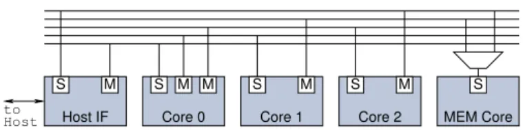
Figure 2: Sample architecture diagram with three compute cores, one memory core and one host interface core
face as the host processor core, but omits the integrated CPU core.
In IMORC, shared memory is modeled as a special kind of core with no execution unit but a large amount of storage. A memory core provides exactly one slave port (see Figure 1c).
Figure 2 presents a sample architecture diagram including three compute cores, a host interface core and a memory core. The host interface core can directly access the slave port of compute core 0, which provides two master ports for access-ing the slave ports of compute cores 1 and 2. These two cores’ master ports access the memory core, and the master port of compute core 2 is additionally connected to the slave port of the host interface core.
3.2. The Execution Model
The intention of the execution model is to specify an applica-tion’s behavior. An application splits into a number of commu-nicating tasks, where each task comprises operations that can be grouped into three distinct but possibly overlapping phases:
• incoming communication: A task receives and processes incoming messages, which typically first specify the pa-rameters of the computing job and then contain the data to be processed.
• local computing
• outgoing communication: A tasks sends messages to other tasks or responds to its invoking task.
Figure 3 shows an example for a task. The tall box in the middle represents local operations performed by the task, the smaller boxes on the left and the right side represent commu-nication points with other tasks. Tasks can communicate with other tasks using messages. Messages can be read (rd) or write (wr), the first kind is used for requesting data from another task, the other one for sending data to another task. Read requests need to be followed by a response message (resp). Tasks can be modeled at different levels of abstraction, depending on the actual requirements. On a rather abstract level, the task compu-tations may be described by pseudo code or a code segment in a high-level language. On a detailed level, the computations may be expressed as a sequence of micro operations or RTL code.
Figure 4 shows a task graph with two tasks accessing a block of shared memory. Modeling memory as separate task simpli-fies the runtime analysis, especially when multiple tasks access a shared block of memory and therefore contention may occur. Additionally, due to the request-response nature of the commu-nication model, tasks operating on streams of data can be mod-eled in natural way. The communication subtasks send read re-quests to the appropriate memory task, and as soon as the data
LOCAL OPS OUTGOING MSG INCOMING MSG wr rd rd resp wr rd resp rd
Figure 3: Diagram of a sample task
MEM TASK TASK 1 TASK 2
TASK 0
Figure 4: Task graph with two tasks accessing a memory task
becomes available the local operation subtasks start processing. Accelerator development in IMORC requires the designer to eventually map the tasks of the execution model to cores of the architecture model. Since IMORC also models host communi-cation and memory access as activities captured by cores, the mapping step actually includes the partitioning between host CPU, FPGA and memories as well as the breakdown of the application’s functionality into communicating cores on the re-configurable fabric.
It has to be noted that the IMORC architecture and execution models are rather general and do not pose any restriction on the behavior of tasks or cores, respectively. For example, there is no need to enforce blocking reads on incoming messages as in the Kahn process network (KPN) model, or to specify rates for the production of outgoing messages as in the synchronous data flow (SDF) model. In contrast to these well-known for-mal models of computation, IMORC provides more degrees of freedom but misses formally provable characteristics.
3.3. Development Flow
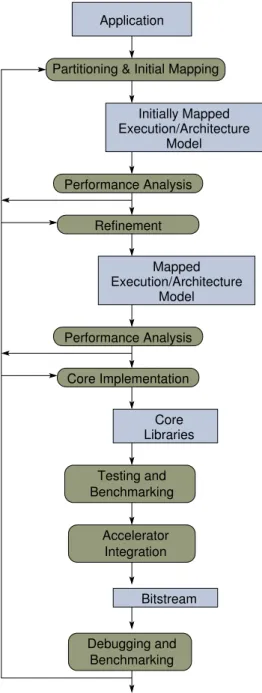
Figure 5 shows the typical IMORC development flow. Ac-celerator development starts out with partitioning and initially mapping the application to the reconfigurable computing sys-tem. In most cases there exists already a software implementa-tion of the original algorithm that can be used as starting point
Mapped Execution/Architecture Model Core Libraries Application Bitstream Model Execution/Architecture Initially Mapped Performance Analysis Refinement Performance Analysis Core Implementation Partitioning & Initial Mapping
Accelerator Integration Testing and Benchmarking Debugging and Benchmarking
CPU Memory FPGA Memory CPU Memory FPGA Memory Processing Post Main Computations Preprocessing Preprocessing Postprocessing Kernels Storage Tasks Partitioned Application Partitioned Application Application
Figure 6: Partitioning and initial mapping of an application
for the partitioning process. To decide which parts of the ap-plication should be accelerated, software performance analysis and profiling tools are employed to identify the computationally most intense application parts (kernels). Subsequently, these kernels are mapped to the FPGA. Since storage access times play a major role in many implementations, the application’s main data structures are extracted into storage tasks. The stor-age tasks can then be mapped to the memories available in the system. Figure 6 demonstrates the partitioning and initial map-ping process.
After partitioning and initial mapping a first performance analysis can be performed, for example by estimating the amount of data to be transferred to the FPGA and back, or from the FPGA to the memories. We usually perform this step manually and estimate communication times by considering the amount of data to be transferred and the maximum available communication bandwidth. Such basic performance analysis can lead to new mappings which, for example, exclude certain kernels from being mapped to the FPGA or use a different map-ping of storage tasks.
In the refinement phase, tasks are broken down to a more detailed level. While for the tasks mapped to the CPU an ef-ficient implementation often exists, tasks mapped to the FPGA have to be split into multiple communicating tasks that actually form specifications for the subsequent circuit design. An essen-tial objective of the refinement step is to extract opportunities for exploiting parallelism. An example for such a refinement is presented in Figure 7. The original task graph on the left con-sists of two tasks, a master and a worker. The master on the left sends data to be processed to the worker. When first set of data has been processed, the results are returned and the next set of data to be processed is transferred. In the refined task graph, instead of waiting for the first set of data to be completely pro-cessed, data is streamed from the master core to the first worker core. This core performs some processing on the data and
for-Figure 7: Example of a refinement by streaming data through a set of tasks
wards the results to another worker core and so on. The last worker core then returns the results to the master core.
Another possible refinement is the extraction of the request subtask and the datapath of a task. In many other models, data is assumed to be directly accessible in constant time, so op-erations are directly applied to data. In the IMORC modeling approach, however, requests for data and processing can be split into separate tasks that get mapped to the same core – tasks re-questing data are mapped to the communication controller of a core, tasks operating on the data are mapped to the execution engine of a core (cf. Figure 1).
Based on the refined execution and architecture models a more detailed performance analysis takes place to get more ac-curate performance estimations. For example, communication estimation now includes the block sizes for data transfers. If the estimated performance is found sufficient, the core imple-mentation phase starts. For each core of the architecture model a corresponding circuit is created or taken from a core library. The individual cores are tested and benchmarked. In the next step, all cores are integrated with the IMORC multi-bus on-chip network infrastructure and synthesized to the accelerator bit-stream. The final accelerator is loaded onto the reconfigurable computer, debugged and benchmarked. The performance mon-itoring infrastructure of IMORC greatly facilitates the analysis of the accelerator behavior and the identification of bottlenecks. Based on such monitoring data, development iterations can be performed in order to optimize the performance. Eventually the IMORC performance monitoring infrastructure can be re-moved.
4. IMORC Architecture Template
As outlined in the previous section, IMORC assumes that an application is decomposed into multiple communicating cores which encapsulate computations as well as access to mem-ory and external communication interfaces. A key element of IMORC is its multi-bus on-chip network for connecting such cores within an FPGA. To achieve high-throughput commu-nication with minimal congestion, IMORC relies on a multi-bus architecture with slave-side arbitration. In this section, we present the basic elements of IMORC and show how accelera-tors architectures with different network topologies are created.
Table 1: Request packet format
CMD command field (RD or WR)
ADDR destination address
SIZE number of 32 bit words to transfer OPT optional information
decoding is up to the designer
4.1. Cores, Links and Channels
IMORC cores access the on-chip communication infrastruc-ture via ports. There exist two types of ports, denoted as master and slave ports. A link between two cores can only be formed by connecting a master with a slave port. IMORC uses unidi-rectional buses and differentiates between commands (requests) and data transfers. Hence, each link splits into three channels, a request channel (REQ), a master-to-slave channel (M2S), and a slave-to-master channel (S2M). The REQ channel is used for transmitting write or read requests from the master to the slave port. Data is transferred from the master to the slave port via an M2S channel, and from slave to master port via an S2M channel, respectively. A link must comprise at least the REQ channel and can, additionally, comprise an M2S and an S2M channel.
Figure 8 details the signals for an IMORC link, basically con-sisting of a data bus and two handshake signals for each chan-nel. The REQ channel uses a data busreqto transmit request packets and the two handshake signals req_wait and req_wr
on the master side or req_rd on the slave side, respectively. Table 1 lists the fields available in the request packets. A re-quest packet specifies the command, write or read, the desti-nation address, the number of words to write or read, and an optional user-defined field. The data to be written or read is then transferred over the M2S and S2M channels. The desti-nation address is interpreted by the slave port. For example, a memory controller core will use the destination address to ac-cess the attached memory, and a compute core could use it to select between a set of internal registers.
IMORC inserts asynchronous FIFOs into each channel which allows for operating each core at its maximal speed in its own clock domain. Particularly, memory cores can operate at their top speed and, possibly, provide sufficient bandwidth to serve several compute cores at once. Moreover, the additional FIFO storage in the network decouples core execution which, depending on the actual application, can help improve perfor-mance.
In case the data bitwidth of master and slave ports differ, IMORC inserts a bitwidth conversion module into the link. The bitwidth conversion modules are placed before the FIFOs, which always have the same bitwidth as the slave ports. The conversion from a wide master word to a small slave word is straight-forward and involves several writes to the FIFO for one word sent by the master. Converting from small master to wide slave words is more complex. In such a case the bitwidth con-version module generates a set of sub-word write enable sig-nals to mask the sub-word within the slave word that is to be written. As a consequence of these bitwidth conversion
mod-REQ M2S S2M BITWIDTH CONVERSION M S CORE #1 CORE #0 REQ M2S S2M PERFORMANCE COUNTERS MONITOR counters perf to other to Host
empty req_wait req_rd req m2s_wait m2s_data s2m_wait
s2m_data
req_wr m2s_data s2m_wait req_wait m2s_wait m2s_wr s2m_rd s2m_data
full
req
m2s_rd s2m_wr
Figure 8: IMORC link with its channels and signals
ules, a compute core with a 32 bit interface can be connected to a memory core with a 64 bit interface, and also to a 256 bit interface without any change in the compute core itself. This greatly facilitates reuse of cores and porting applications to dif-ferent accelerator platforms. The integration of the FIFOs and the bitwidth conversion module into an IMORC link is shown in Figure 8.
4.2. Network Topology and Arbitration
An application typically comprises several IMORC cores connected in a certain topology. Each core can have an arbi-trary number of master and slave ports, hence, connecting mas-ter and slave ports in a 1:1 fashion is basically sufficient to build arbitrary topologies. However, as this approach requires cores with a rather high number of master and slave ports, IMORC supports 1:n, m:1, and m:n connections as well.
A 1:n connection allows a master port to address several slave ports at once. To this end, the signalsreq_wr andm2s_wrare turned into vectors. By selecting a subset of these write en-able signals, the master may issue multi-cast or even broad-cast request messages and data writes. The wait signals from the individual FIFOs also form a vector and are routed back to the master port. IMORC even supports the S2M channels in a 1:n connection with the restriction that a master can address only one FIFO to read from at any time.
An m:1 connection allows a slave port to be driven from several master ports. IMORC employs slave-side arbitration and inserts an arbiter module right before the slave port. Fig-ure 9 displays the IMORC interconnect for a 2:1 connection. In this figure, the optional bitwidth conversion modules are omit-ted for the sake of readability. The arbiter contains FIFOs for
REQ, M2S, and S2M channels from each master port. A se-lector module SEL in the REQ channel decides which request is served next. By default the selection is done in round-robin manner but can easily be changed as needed, for example to introduce priorities. Once a request is being processed, the cor-responding M2S or S2M channel in the arbiter is activated to read or write data, respectively. If required, m:1 and 1:n pat-terns can be combined to form an m:n connection.
4.3. Monitoring Infrastructure
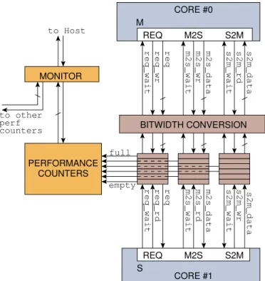
Optimizing the performance of an application consisting of multiple cores is not a trivial task and requires to balance com-putation speed with communication bandwidth, and to mini-mize contention for shared resources, e. g., external memory. While the IMORC architectural template offers the designer the freedom to address performance problems, e. g., by increas-ing data widths, replicatincreas-ing compute cores, replacincreas-ing a compute core with a higher throughput version, selecting the appropriate remedy requires information about the dynamic behavior of the application. To this end, IMORC provides performance coun-ters attached to the FIFOs within the links and arbiter modules. For each FIFO, the number of full and empty events is counted as shown in Figure 8. In user-defined time intervals a monitor-ing core triggers async_and_resetsignal that tells the perfor-mance counters to sync the current counter value into a register in the monitoring core’s clock domain and to reset the counter. The synchronized values can then be sequentially read by the monitoring core using a shared bus.
In user-defined time intervals the performance counters are read and reset, and the event counts are collected by a monitor-ing core. Since the cores can operate in different clock domains, the pure number of events is not sufficient to draw conclusions about the overall system. Hence, each performance counter ad-ditionally employs a cycle counter that is incremented every clock cycle. Using the performance counter infrastructure, de-signers can monitor the dynamic behavior of an application and gather information about the cores, e.g., when they start or stop processing and how much bandwidth they produce on the dif-ferent channels. In our current implementation, the monitoring core is accessed from outside the FPGA via a JTAG port, which is a highly portable approach that has the benefit of not affecting the timing of monitored system.
4.4. Infrastructure Cores
Besides the on-chip interconnect, IMORC also provides sev-eral infrastructure cores such as memory controllers, a host in-terface core, IMORC-to-Register inin-terface cores, request gen-erator cores and farming cores. These cores provide function-alities often needed and are available to assist the designer in generating accelerators.
Memory interface cores. IMORC provides memory cores for accessing on-chip, off-chip and host memory. Access to these three kinds of memory is completely transparent to the accel-erator cores. From an execution core’s perspective, there is no functional difference between on-chip, off-chip and host mem-ory, which greatly eases design space exploration. The IMORC
interface to on-chip memory is written completely in synthesiz-able VHDL and wraps and extends availsynthesiz-able vendor memory cores. Current vendor implementation tools are only able to in-fer simple types of on-chip memory from VHDL, such as sin-gle port or dual port memory without byte-enable signals. For high speed access wide memories are preferable, making sub-word writes necessary. Furthermore, IMORC also wraps and extends vendor cores for accessing off-chip memory to allow for an integration of these cores into the IMORC’s on-chip net-work. Many host interfaces, e.g., PCI, PCIe, HyperTransport, support master transfers to host memory. Using an appropriate interface, such memories can be accessed by IMORC. IMORC does not limit the number of memory interface cores that can be used in a system. The maximum number of supported cores ba-sically depends on the number of available off-chip and on-chip memory resources as well as on the number of logic resources available on the target device. Instantiating vendor cores makes the IMORC infrastructure for accessing memory vendor spe-cific.
Request generator cores. Request generator cores are basically pre-defined implementations of the REQ CTRL modules (dis-played in Figure 1a) for certain request sequences. Instantiating and configuring request generators relieves the designer of cre-ating such logic by hand each time. The streaming request gen-erator is a basic module which is configured with a command (read or write), a base address, the amount of data to be trans-ferred and the size of each request. Sending requests can be in-terrupted, for example when different requests are to be inserted by other request generators. Additionally, the core can be con-figured with a step parameter to increment the base addresses of the requests by a user-defined value. This is highly useful, for example, for accessing the diagonal elements or a diago-nal band of a matrix. A more sophisticated request generator can inject a sequence of read and write requests into a channel. Different base addresses, amounts of data and request sizes can be set for read and write requests. The sequence of reads and writes can be programmed by two further parameters, encoded as bit vectors. The first one represents the initial sequence, that is performed once when the request generator starts. The sec-ond sequence is repeatedly executed after the setup phase. Such a setup phase is useful when data is to be read, processed and written back to memory - in this case, the datapath pipeline first gets filled before data is written back. A third example of a re-quest generator posts a sequence of read and write rere-quests, but does not execute a static sequence. Instead, the request gener-ators monitors thewrsignal of the M2S channel. When a con-figurable amount of data is sent to this channel, an appropriate write request is inserted into the sequence of read requests. IMORC-to-Register/Register-to-IMORC interface cores. Exe-cution cores usually need to be configured with parameters specifying, for example, the start address of data to be pro-cessed and the amount of data to be propro-cessed. Typically, these parameters are packed into a job message that is to be decoded by the execution core. The IMORC-to-Register (I2R-IF) inter-face core is an infrastructure core that performs the decoding
wr data
full full wr data
req req data rd empty data rd data wr full
rd rd empty empty wr wr full full
d en empty empty empty req rd rd en d rd data wr full SEL dec M CORE #1 M REQ M2S S2M S2M M2S REQ REQ M2S S2M CORE #2 S CORE #0
Figure 9: Arbitration module for a 2:1 connection
of job messages. The core provides a configurable amount of internal registers that can be accessed in two ways: First, mes-sages appearing on an IMORC slave interface are decoded and the appropriate read/write operations are performed on the reg-ister block. Second, a separate interface provides direct
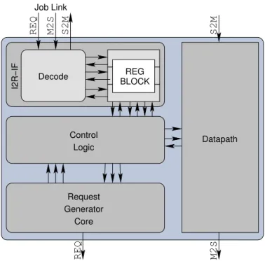
read-/write access to the registers. One of the registers can option-ally be declared as state register, which blocks the IMORC link when containing a non-zero value. For example, a core can send a job message to such an I2R interface core and set the state reg-ister to ’1’. Consequently, the I2R interface will not accept any further transfers on the IMORC link. The slave core then starts processing and resets the state register when finished. Now, further job messages can be accepted on the IMORC link. This way, cores sending jobs to other cores are not required to al-ways check if the other core is currently idle – jobs can be sent as long as the corresponding link’s FIFOs are not full. Since the state register blocks all requests, the I2R interface will also not respond to any read requests during that time. Since all re-quests are processed in-order, several job messages following a read will result in a read response on the S2M channel not be-fore all jobs are finished – this way a core can even synchronize with the finalization of the jobs sent to another core. IMORC further inserts a performance counter into the state register of the I2R interface core for monitoring the runtime of the core. Figure 10 shows a sample core using the IMORC-to-Register interface core. A master core can send a job description to the I2R-IF. The register interface can be directly connected to one or multiple request generator cores, providing a straightforward
M2S REQ S2M S2M REQ M2S Datapath Request Generator Core Logic Control I2R−IF REG BLOCK Decode Job Link
Figure 10: Sample core using the IMORC-to-Register interface core
method for generating the control unit of a core. Additionally, IMORC provides a Register-to-IMORC interface, which also implements a set of directly accessible registers connected to an IMORC link. However, this time the interface is an IMORC master. This interface can for example be used for generat-ing job messages and sendgenerat-ing them to a compute core’s I2R-interface using an IMORC link.
Farming cores. Besides streaming, farming is another recur-ring design pattern in parallel programming. Data is partitioned and distributed among multiple processing elements (workers). Each processing element operates autonomously on its own set of data. This design pattern is supported by IMORC by pro-viding a dedicated job scheduler - the farming core. Configu-ration parameters of the farming core are the format of the job description (number and size of registers) and the number of worker cores. The farming core receives job messages on an IMORC slave port and forwards them to the worker cores. Ad-ditional to job messages, the farming core can respond to sta-tus requests. Such request messages are useful for probing the execution status of workers and synchronizing with the com-pletion of all worker cores. The request message can be block-ing or non-blockblock-ing. Non-blockblock-ing requests are immediately answered and specify which cores are idle and which are still processing. Blocking requests are answered as soon as all jobs have been finished.
4.5. Accelerator Generation and Portability
The IMORC architectural template is completely written in synthesizable VHDL. Specifically, the FIFOs are implemented based on the techniques described in [22] without using any architecture specific components, making IMORC a vendor-neutral tool. While currently we have only evaluated IMORC on the XD1000 platform (see Section 5), these properties make porting IMORC applications to new architectures rather sim-ple. One has to implement a host interface core and appropriate memory interface cores for the concrete target architecture and then can remap the application to the new architecture.
Before synthesizing an application to an FPGA target the de-signer can tailor the IMORC architectural template to match the requirements of the application. Configurable parameters in-clude for example the data widths of the channels for each mas-ter and slave port, FIFO depths, the number of masmas-ters for each arbiter, etc. To minimize resource overheads, the actually syn-thesized IMORC infrastructure is application-specific, i.e., only the required channels, arbiters and bitwidth conversion mod-ules are inserted into the design. The decision which design units are required is taken based on the parameters specified by the designer. If, for example, the master’s and slave’s bitwidth are equal, the bitwidth conversion modules are not required and are automatically removed from the design. The generation of unnecessary channels can be either avoided by configuring the actually required number of ports using a VHDL generic pa-rameter or the developer can leave unused ports open and rely on the synthesis tool to remove any unused logic.
5. XD1000 Platform Support
This section presents an overview of the XtremeData XD1000 reconfigurable workstation and the IMORC cores that have been developed as platform support. The XD1000 is a dual socket system where one of the sockets is equipped with a 2.2 GHz AMD Opteron processor, and the other one with a module featuring an Altera Stratix II EP2S180-3 FPGA. Phys-ically, the FPGA is connected to the processor using a 16 bit HyperTransport link with 800 MT/s, which results in a rather low latency communication at a theoretical peak bandwidth of about 1.6 GB/s in each direction. Furthermore, the XD1000 system comes with 4 GB of main memory (DDR SDRAM) for each the Opteron and the FPGA.
5.1. IMORC HyperTransport interface
For communication to the host CPU and memory, IMORC provides an interface to HyperTransport which is based on the HT cave described in [23]. The HT cave and our IMORC in-terface support communication initiated by the host as well as communication initiated by IMORC cores. HT packets consist of a header containing control information that is optionally fol-lowed by a certain amount of data. Fundamental elements of the header are the packet type (byte/dword read/write, broad-cast, etc.), a mask/count field, a tag, an address and several other fields. HyperTransport uses virtual channels for commu-nication, “posted” for requests not requiring a response, “non-posted” for requests expecting a response and “response” for responses. Each of these channels exists once per direction. Re-sponses are related to the original non-posted request by copy-ing the tag field.
The HT cave maps three distinct address regions (BARs) of the FPGA into the host processor’s address space. HT pack-ets sent by the host are decoded, packet headers are written to separate FIFO interfaces for posted and non-posted requests, data is also written to FIFO interfaces. Our IMORC interface decodes the packet headers. Packets targeting one of the first two address regions are converted into IMORC requests and forwarded to two distinct IMORC links. Data corresponding to the HT packets is also forwarded to the M2S channel of the appropriate link. For reads, the tag and count field and the ID of the IMORC link used is forwarded additionally to a response datapath using a FIFO. As soon as data becomes available on the appropriate IMORC link’s S2M channel, an HT header con-taining the original tag and count field is sent to the HT cave’s response FIFO and the data is forwarded to the data FIFO.
The third address region directly accesses an embedded block of memory, used as page mapping table which maps host memory into the address space of a third IMORC link. For this purpose, the page mapping table needs to be filled with phys-ical page addresses of the target host memory by the user ap-plication. When cores send requests over this IMORC link, the upper bits of the IMORC request form an index into the page mapping table, the lower bits are the offset into the page. Using this address mapping, the IMORC packet is converted into an equivalent HyperTransport packet and posted to the appropriate virtual channel’s FIFO interface of the HyperTransport cave.
For read requests, the tag field is incremented with each request posted. Since HyperTransport supports out of order responses, the response datapath possibly has to reorder these responses. For this purpose, it contains a block of embedded memory for each tag, which can store one full-sized HT data packet. Re-sponses arriving on the HT are first written into the appropriate memory block, and the block is marked as valid. The TAG is marked as free, enabling the request block to reuse it for an-other HT read request. A separate logic waits until the data block for the first tag is valid. Then, data in this block is for-warded to the S2M channel of the IMORC link, the data block is marked as invalid and the logic waits for the next tag’s data block to become valid. Additionally, the third IMORC link can be used for sending interrupt messages to the host CPU. Writes to a configurable address on this IMORC link are converted into an HyperTransport interrupt message that is sent to the host.
Table 2 lists the resource requirements of the HT interface core. The number of used block memory resources (M512, M4k and M-Ram) mainly depends on the amount of host mem-ory that is mapped into the FPGA’s address space, e. g., the size of the embedded page mapping table. The core’s user interface may be operated at up to 200 MHz, enabling accelerators to uti-lize the maximum bandwidth delivered by the HT interface.
5.2. Interface to the DDR SDRAM
For off-chip memory access, IMORC wraps the Altera DDR SDRAM controller core which can access memory in blocks of configurable burst sizes. DDR SDRAM writes always cover a complete burst, i.e., 2, 4 or 8 clock cycles, depending on the controller configuration. The XD1000 system provides a 128-bit-wide memory. Hence, depending on the burst size, 256 bit, 512 bit or 1024 bit are written to memory during a trans-fer. Since the XD1000 does not provide data mask pins for the memory to mask out bytes not to be written during a burst, IMORC implements a read-modify-write cycle for writes that do not match one of the burst sizes. The read-modify-write cy-cle incurs overhead but at the same time increases flexibility and potential for core re-use, as the core designer is not necessar-ily bound to pre-determined burst sizes and link widths. Table 2 lists the resource requirements of the DDR SDRAM inter-face core that includes the Altera DDR SDRAM controller core and the interface to IMORC. The IMORC interface of the DDR SDRAM interface core is operated at the same clock frequency of 166 MHz as the DDR memories, so the full bandwidth of the memories can be utilized.
6. Case Study
We demonstrate the IMORC workflow and benefits on the detailed example of developing a hardware accelerator for the k-th nearest neighbor thinning problem on the XtremeData XD1000 system [1]. In this section, we present the k-th nearest neighbor thinning problem and the application-specific IMORC cores that are derived from it.
6.1. k-th Nearest Neighbor Thinning
k-th-nearest-neighbor (KNN) methods are omnipresent in many areas of science and engineering. In statistics and data analysis, for example, KNN techniques play an important role for the non-parametric estimation of density functions from data samples [24]. Given a set ofndata samples, where each sampleiis ad-dimensional vector, an Euclidean distance metric σiis computed for any pair of samples. For each data sample, the resulting n distance values are sorted in ascending order, i.e.,σ1
i ≤σ 2
i, . . . ,≤σ n
i. A KNN density estimate ˆf(i) can then be formulated by setting: ˆf(i)∝1/σki.
The parameterkis typically chosen ask≈ √n[25]. Thus, the local density around each data sampleiis estimated by the reciprocal of the distance to thek-th nearest neighbor. In other words, a low density means that ad-dimensional sphere with data sampleiat its origin has to be rather large in order to con-tainkdata samples.
The KNN approach is also widely applied for solving clas-sifications problems, such as in machine learning, data mining and stochastic optimization [26]. There, a KNN classifier re-quires a labeled training data set consisting of d-dimensional feature vectors and their class labels. In order to classify a new feature vector, theknearest training vectors are determined ac-cording to some distance metric. Often, a reduction of the size of data samples is desired to reduce both the classification time and the memory required to store the data set. Many reduction techniques fall into the category of condensing or thinning ap-proaches, [27], that aim at properly selecting a subset of training vectors from the original data set.
Recently, some methods related to KNN-based thinning have been successfully accelerated with FPGAs. For exam-ple, Yeh et al. present a KNN classifier [28] that operates in the wavelet domain and uses partial distance search to acceler-ate the classification process. The resulting architecture is in-tegrated as a core with the Altera NIOS CPU softcore. In [29] Chikhi et al. present an FPGA accelerated KNN classifier for content-based image retrieval that achieves a speedup of 45x over a software implementation. Also the related k-means clus-tering method has been successfully accelerated in reconfig-urable hardware. For example, Saegusa and Maruyama have presented an architecture [30] that can perform k-means clus-tering on video data in realtime.
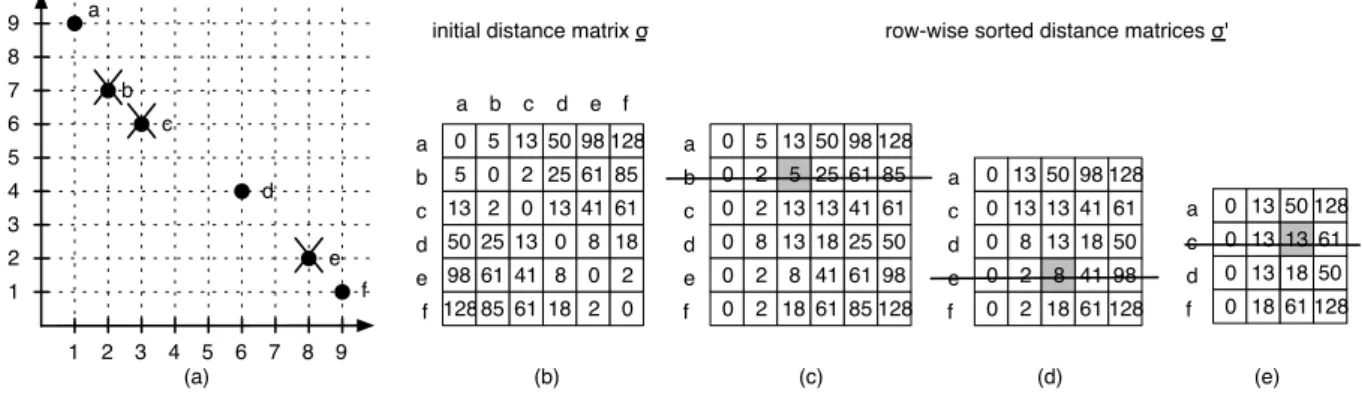
The KNN-based thinning method we are targeting in this work takes a set of input vectors and searches for the subset of vectors that represents the distribution of the original set the most representative. The KNN thinning procedure, shown in Algorithm 1, is called with a setPof differentd-dimensional vectors pi = (pi1,pi2, . . . ,pid) andN, the targeted cardinality ofP, and successively eliminates vectors with the shortest Eu-clidean distance to their neighbors until Phas been reduced toN elements. In each iteration, the algorithm first constructs a distance matrixσ = (σil) from the pair-wise Euclidean dis-tancesσilbetween all vectors. Sortingσrow-wise in ascending order defines sorted distance vectorsσi0of lengthm. While
ini-tially equal to|P|, the number of vectorsmis reduced by one in each iteration. Now, the algorithm iterates over all columns
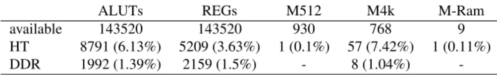
Table 2: Resource requirements for the HyperTransport interface core and the DDR SDRAM controller core on an Altera Stratix II EP2S180 FPGA
ALUTs REGs M512 M4k M-Ram
available 143520 143520 930 768 9
HT 8791 (6.13%) 5209 (3.63%) 1 (0.1%) 57 (7.42%) 1 (0.11%)
DDR 1992 (1.39%) 2159 (1.5%) - 8 (1.04%)
-ofσ0. Starting with columnl=3, the rowsσ0
i with minimum distance valuesσ0
ilamong all distances in columnlare selected and assigned to setM. If the minimum is unique, the respec-tive row σ0
i ∈ σ
0 as well as the corresponding vector p i are deleted which reduces the set of vectorsP. If the minimum is not unique, the next column ofσ0is considered which corre-sponds to checking the distances to the next closest neighbors. If no unique minimal distance is found for all columns of σ0, an arbitrary row having a minimal distance value in the last col-umn is deleted. Obviously, the first two colcol-umns never need to be considered since each vector has a distance of 0 to itself (first column) and the distances between pairs of vectors are symmetric (second column).
Algorithm 1KNN thinning algorithm 1: procedureKNN_thinning(P,N) 2: while|P|>Ndo 3: compute/updateσil← q Pd j=1(pi j−pl j)2 4: ∀rows ofσ:σi0←sort(σi) 5: forl←3, . . . ,mdo 6: M ← {σ0 i | ∀σ 0 jl:σ 0 il≤σ 0 jl} 7: if|M|==1then 8: break 9: end if 10: end for
11: delete arbitrary rowσi∈ Mfromσ0
12: P ← P \ {pi}
13: end while 14: end procedure
The operation of the KNN-based thinning algorithm is illus-trated in the example shown in Figure 11. The initial population of six 2-dimensional vectors as well as the three vectors that are discarded by three iterations of the thinning algorithm are shown in Figure 11(a). The distance matrixσfor the first iter-ation is presented in Figure 11(b), and the row-wise sorted dis-tance matrixσ0in Figure 11(c). Note that the matrices actually show the square distances which is sufficient for this algorithm. A unique minimum is found in the third column which leads to the deletion of rowbfrom the matrix and vectorbfrom the population, respectively. In the second iteration, the distance matrix is updated and re-sorted which results in the matrix of Figure 11(d). Again, a unique minimum is identified in the third column and, consequently, roweand vectoreare deleted. Finally, the third iteration leads to the deletion of vectorc. 6.2. Mapping of KNN to IMORC and Refinements
In this section we discuss the mapping of the KNN thinning application to the IMORC architecture and present the
refine-ments we make during this process. As visible in Figure 5, the design flow usually starts with partitioning and initial mapping of the application. The partitioning phase hereby consists of benchmarking and profiling the application for extracting the most compute intense parts of the application, which are then initially mapped to the FPGA. Different tools can be used for the profiling procedure, such as, GProf [31], Valgrind [32], or OProfile [33]. However, in this case study we do not concen-trate on a large application from which only parts are to be ac-celerated, but the focus lies on the KNN thinning procedure that is to be completely implemented on the FPGA. The KNN procedure will typically not be executed as an isolated applica-tion, but as a kernel in a larger application. Since it is already clear that the complete KNN kernel is to be implemented on the FPGA, the partitioning phase is omitted in this case study and the design process starts with the initial mapping phase. 6.2.1. Initial Mapping
For mapping the KNN thinning application to the IMORC ar-chitecture template, we need to decompose the application into a set of communicating tasks which will be mapped to IMORC cores later on. In addition to the decomposition of the function-ality into tasks, we can already determine which tasks could be potentially executed in parallel or in a pipelined fashion at this early stage of the design process. As the algorithmic core of our application is well described in a formal way we can derive much of this information from analyzing Algorithm 1.
We can see, that the algorithm can be broken up into five major tasks:
• distance calculation: computing the distance values (line 3 of Alg. 1)
• sort: sorting the distance values (line 4)
• search: searching for the vector with minimum distance (lines 5–10),
• discard: discarding this vector from the distance matrix (line 12), and
• ctrl: controlling the iteration of this process until the num-ber of vectors has been reduced to a target numnum-ber (line 2).
Further, we can identify two main data structures that are needed by the application, which will also be modeled as IMORC tasks:
• VM: a memory for storing all vectors, and
• DM: a memory for storing the results of the distance com-putation.
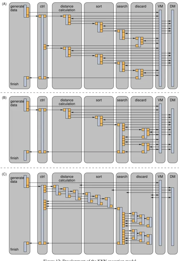
The interaction of the cores in this initial application map-ping is shown as a task graph in Fig. 12(a). This figure also shows a data generation task that is executed on the host CPU
row-wise sorted distance matrices σ' 0 5 13 50 5 0 2 25 13 2 0 13 50 25 13 0 a b c d a b c d 98 61 41 8 128 85 61 18 98 128 61 85 41 61 8 18 0 2 2 0 e f e f 0 0 0 0 5 2 2 8 13 13 13 50 25 13 18 a b c d 98 61 41 25 128 85 61 50 0 0 2 2 8 18 41 61 61 85 98 128 e f 5 0 0 0 13 13 8 50 13 13 98 41 18 a c d 128 61 50 0 0 2 2 18 41 61 98 128 e f 8 f c b a d 4 3 2 1 1 2 3 4 8 7 6 5 5 6 7 8 9 9 e
initial distance matrix σ
(a) (b) (c) (d) 0 0 0 13 13 13 50 a c d 128 61 0 18 61 128 f 13 18 50 (e) Figure 11: Example for the KNN-based thinning algorithm in two dimensions: thinning 6 vectors to 3 vectors
and is triggering the KNN controller task.
6.2.2. Refinement #1: Compute Distances Just Once
At this stage in the design process, we take two decisions af-fecting the accelerator architecture. First, to reduce the amount of computations we decide to move the computation and sorting of distance values out of the loop in Algorithm 1 and compute the sorted matrixσonly once. This is made possible by storing with each distance valueσilthe indices of the two vectors for which the distance has been computed. The discard task now not only operates on the original vector table but also on the distance table for removing all references to the vector to be discarded.
This modification increases the size of the distance table and therefore also increases the runtime for the distance calculation, the sort task, and the discard task, which now has to process the complete distance table. However, the distance calculation and the sort tasks are now only executed once, which reduces the overall runtime. In essence, we trade an increased memory requirement for improved performance with this refinement.
The interaction of the cores in the refined mapping is shown as a task graph in Fig. 12(b).
6.2.3. Refinement #2: Exploit Parallelism with Farming Cores The next refinement step is guided by the observation that the distance computation between two vectors and sorting the rows of the distance matrix (lines 3 and 4 in Algorithm 1 are well amenable for parallelization. To exploit the available par-allelism we can use IMORC’s farming capabilities to distribute the tasks of distance calculation and sorting to several identical subtasks that perform the actual operation.
In this refinement, each distance calculation task is respon-sible for calculating the distances of exactly one vector to each other, hence calculating one row of the distance matrixσ. The same refinement is done for the sorter task, each one sorts one row ofσ. Each distance calculation task starts the correspond-ing sorter task upon finishcorrespond-ing. However, since the search and discard tasks may not be started before all distance calculation and sorter tasks are finished, the sorter tasks are not allowed to directly start the search and discard task. Instead, an additional control task is inserted to synchronize the finishing of the sorter
tasks. The interaction of the cores in the refined mapping is shown as a task graph in Fig. 12(c).
While it is clear that this refinement may improve the overall performance the impact of increasing the number of distance calculators and sorters used by the farming cores is not evi-dent. Even for a comparatively simple application like KNN thinning, the interaction between cores, the delays introduced by competing for shared resources or the input-specific pro-cessing times (the minimum computation in this case), make an analytical performance modeling difficult. Hence, to find a suitable number of distance calculation and sort tasks we eval-uate the implementation with test sets whose runtime behavior is analyzed with IMORC’s performance counters.
We use the performance counters for measuring the number of full and empty events that happen on the corresponding FI-FOs in the IMORC links during each phase of the KNN algo-rithm. For example, if a FIFO in the S2M channel frequently runs full and the corresponding M2S FIFO runs empty, the re-spective core is known to be compute-bound. In that case we apply farming and add more compute cores for the correspond-ing task for maximizcorrespond-ing throughput. Conversely, if the S2M FIFO frequently runs empty and the M2S FIFO often runs full, the task is certainly memory-bound. Hence, the number of pro-cessing cores used in farming may be reduced without an im-pact on the overall performance.
The availability of performance counters allows us to mea-sure such information for a large set of realistic test sets during execution. Much like established profiling tools for software, IMORC provides runtime statistics and allows for identify-ing bottlenecks in more complex accelerator architectures with data-dependent behavior. It must be emphasized that IMORC monitors the running accelerator in real-time instead of a lation model. For example, our experiments with VHDL simu-lations of the KNN accelerator for|P|>128 andd =32 have shown that we need 8.6×10⁶ clock cycles on the simulating machine for one cycle of the simulated accelerator. Simulating VHDL models of the KNN accelerator with realistic workloads thus takes days.
6.3. Implementation of KNN Cores
After the application has been decomposed into a number of communicating tasks in the application mapping phase that has
finish finish finish (C) (B) (A) DM VM DM VM DM VM generate data
ctrl sort search discard
ctrl sort search
ctrl sort search discard
generate data generate data distance distance distance calculation calculation calculation discard
Subtract Square Accumulate WR−Request Generator Core baseaddr size reqsize start finish baseaddr size reqsize start finish finish n start d finish CTRL s2m_data s2m_rd DIM COUNT BUFF dim wr wait wait data data wr wr req_rd req
req_wait m2s_data m2s_rd m2s_wait
s2m_data s2m_wr s2m_wait req req_wr req_wait req req_wr
req_wait m2s_data m2s_wr m2s_wait RD−Request Generator Core IMORC−to−Register Interface Core
Figure 13: Block diagram of the distance calculator
been discussed in the previous section, each of the tasks needs to be implemented as IMORC core. In the following we discuss the architecture and implementation of these cores.
6.3.1. Distance calculator core
The computation of the Euclidian distances, line 3 in Algorithm 1, is wrapped into a distance calculator core (cmp. Fig. 13). We omit the square root function as squared values are sufficient for comparing distances. The distance cal-culator core computes one row of the distance matrixσion each invocation, which allows us to exploit parallelism by instantiat-ing several such cores.
To receive job messages, the distance calculator core con-tains a slave port, connected to an I2R interface core. A job message comprises the base address of the vectors in vector memory, the number of vectors and dimensions, mandd, the indexiof the vector for which the distances to all vectors have to be determined, and the address in distance memory whereσi is to be stored.
Two request generator cores are connected to the I2R inter-face core, the first one sending read requests to the vector mem-ory, the second one for sending writes to the distance memory. The read request generator is first configured for retrieving the vectorifrom vector memory. When finished, it is reconfigured for issuing read requests to fetch all vectors. At the same time, the second request generator is configured for sending write re-quests to the distance memory for storing the distances.
The datapath reads the first ivector’s coordinates from the vector memory’s S2M-channel and stores them into an internal buffer. Further coordinates are subtracted from the appropriate coordinates in the buffer, the coordinates distances are squared and added up. The resulting distances are sent to the distance memory’s M2S-channel.
When all distance values are written back, the sorter job gen-erator is started, generating a sort job for the computed dis-tances. The I2R interface core is then set IDLE for accepting further distance calculation jobs or state request messages.
6.3.2. Sorter core
For the sorting step, line 4 in Algorithm 1, we use a variant of bubble sort. On each invocation, the sorter core sorts one rowσi of the distance matrix, again allowing to exploit parallelism by instantiating several sorter cores. The job messages are received via a slave port and comprise the number of vectorsmand the base address of σi in distance memory. The job message is decoded in an I2R interface core.
Then, the core proceeds as follows: In the first iteration, a request generator is configured for readingmelements ofσi, i. e., the complete row from distance memory and for storing the same amount of data back to the same location. The dat-apath stores the first element received on the S2M channel as the current maximum. If the next element is smaller than or equal to the current maximum, it is directly forwarded to the M2S channel. Otherwise, it becomes the new current maxi-mum and the previous maximaxi-mum is sent to the M2S channel. At the end of the iteration, the current maximum is written to the M2S channel. Additionally, we remember the positionlof the last element inσi that has been moved left. Thus, in the next iteration onlylelements ofσiare to be streamed through the sorter core. So, the request generator core is reconfigured for reading and writinglelements. This procedure is repeated until the complete row is sorted.
At this point, the state register of the I2R interface core is reset, so that further sort jobs can be processed or occurring state request messages can be responded.
6.3.3. Search core
The search core implements lines 5–10 of Algorithm 1 and is invoked with a job message specifying the total number of vectorsm, the dimension of the vectors and the goal to achieve (e. g.the number of vectors not to discard). The job is decoded in an I2R interface core. A controller transforms these values into input data for an IMORC request generator, which gen-erates read requests to the elements in the third column of the sorted distance matrix. Since data is stored row-wise,mrequest with a size of 64biteach have to be generated, with an offset of m×8byte.
The datapath receives the values from the distance memory, finds the minimum and the information if this minimum was seen more than once. If no unique minimum was found, the controller instructs the request generator to generate requests for the next column. This procedure repeats, until a unique minimum is found or until all columns were searched.
When finished, discard jobs are generated, one for each row of the distance table. The controller waits until all discard jobs are finished and, if the configured goal is not achieved yet, starts the next search iteration.
Table 3: Parameters of the discarder’s request generator
idc,mcur∧idc,iddisc idc=mcur−1 idc=iddisc
rd_base: idc×morig idc×morig (mcur−1)×d
rd_size: mcur mcur d
wr_base: idc×morig iddiscard×morig iddisc×d
wr_size: mcur−1 mcur−1 d
6.3.4. Discarder core
The discarder core implements lines 11–12 of Algorithm 1 and is invoked with a job message specifying the total original and current number of vectorsmorigandmcur, their dimensiond, the ididdiscof the vector to discard and the ididcof the current vector (or row in the distance matrix) to process.
A read-write request generator is configured with the main parameters as defined in Table 3. Three different cases exist: idc,mcur∧idc,iddisc the requests target the distance
mem-ory, readingmcurdistances and writingmcur−1 distances back into the same row.
idc=mcur−1 the requests also target the distance memory, reading and writing the same amount of data as in the pre-vious case. This time, the writes do not target the the same row as the writes, but the row where the distances origin at vectoriddiscreside.
idc=iddisc in this case, the requests target the vector memory, reading all coordinates of the last vector (mcur −1) and storing them to the location where the coordinates of vec-toriddiscreside.
With these parameters, the vector with ID iddisc is replaced with the last vector in the vector table as well as in the dis-tance table. Since the id of the last vector is now changed, the datapath has to perform this change in the distance table’s en-tries, too. The datapath connected to the distance memory’s link reads data from the S2M channel and compares the IDs prepended to the distance value toiddiscand tomcur−1. Every entry with an ID equal toiddiscis discarded, every ID equal to mcur−1 is replaced byiddisc. Entries not discarded are then writ-ten to the M2S channel. The datapath connected to the vector memory’s link only forwards all values from the S2M channel to the corresponding M2S channel.
6.3.5. Controller core
The controller core is responsible for sending job requests to the appropriate cores. A IMORC2Register interface core is used for decoding job messages received from the host. When such a message arrives, the distcalc job generator calculates parameters for n distance calculation jobs and sends them to the distance calculators using a REG2IMORC interface core. When all jobs are sent, a read request is sent to the distance cal-culators for being informed when all jobs are finished. Then, the sort waiter is started. Since sort jobs are directly generated and sent to the sorters in the distance calculators, this core only sends a read request to the sorter cores for getting their finish-ing time. Then, the search job generator generates parameters for the search module, sends them to the search core using the
REGS2IMORC DISTCALCJOBGEN
SORT WAITER SEARCH JOBGEN REGS2IMORC REGS2IMORC Interrupt Generator DISTCALCS JOB LINK start n start start start SORTERS JOB LINK JOB LINK SEARCH HOST LINK dim goal JOB LINK FROM HOST IMORC2REGS
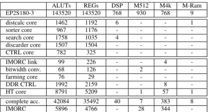
Figure 14: Block diagram of the controller core Table 4: Resource requirements for the accelerator
ALUTs REGs DSP M512 M4k M-Ram EP2S180-3 143520 143520 768 930 768 9 distcalc core 1462 1192 6 - - 1 sorter core 967 1176 - - - -search core 1758 1035 4 - - -discarder core 1507 1504 - - - -CTRL core 782 325 - - - -IMORC link 99 226 - - 4 -bitwidth conv. 68 126 - 2 - -farming core 76 29 - - - -DDR CTRL 1992 2159 - - 8 -HT core 8791 5209 - 1 57 1 complete acc. 42084 35492 40 7 383 8 IMORC 5896 4766 - 28 344
-REG2IMORC interface core and again waits for completion. Last, the interrupt generator core is started, sending an interrupt message to the host link, informing the host that the current job is finished.
Figure 14 shows a block diagram of the controller core. Most of the controller core could be implemented using the existing IMORC supporting cores, only a few lines of additional HDL code had to be written for calculating the correct job parame-ters.
6.4. Numeric evaluation
Using the cores presented in the previous section, we gener-ate a configurable accelerator for the XtremeData XD1000 sys-tem. The number of distance calculators, sorters and discarder cores in the accelerator is configurable, job distribution is per-formed using the IMORC farming cores. All slave arbiters ex-cept that for the sorter job messages use the default round robin port scheduler. The sort job slave arbiter uses a modified port scheduler, which tries to select one of the links from the dis-carder cores in round robin manner first, and only selects the link from the controller core if all other links are empty. This way, the final status request from the controller is ensured to be posted to the farming core last, when all job messages are already forwarded to the sort compute cores. Figure 15 shows the IMORC diagram of the complete accelerator with each two distance calculators, sorters and discarder modules.
S M HyperTransport CORE S M CTRL S DDR CTRL S M FARMING (DISTCALC) S M FARMING (SORT) M S FARMING (DISCARD) M M S M M S M M S M S M S M M M S M M M S DISCARD DISCARD SEARCH SORTER SORTER DISTCALC DISTCALC
Figure 15: Architecture diagram of the accelerator with two distance calculators/sorters/discarders mapped to the XD1000
Using this mapping, we generate accelerators with different configurations (indicated as (ndistcalc×nsort×ndiscard). Table 4 shows the resource usage of some basic elements of the ac-celerators. The last two rows represent the resources used by the complete accelerator and the resources used for the IMORC communication infrastructure of the complete accelerator in the (6 ×6×6) configuration. The communication infrastructure hereby takes about 14% of the overall logic resources.
Figure 16 and Table 5 show the speedups these accelera-tors generate over an optimized software solution that utilize the host CPU of the XD1000 workstation only. The reported speedups are application-level speedups, that is, all overheads for data transfers are included. The test sets were executed with test vectors in 32 and 128 dimensions. The initial data set con-sisted of 32 to 1024 vectors that were thinned to 1/4 of the original set of vectors (i. e., 3/4 of the original data set was dis-carded). Vector coordinates and distance values were stored in 32 bit fixed point representation, the vector ids prepended to the distance values were stored in 16 bit unsigned integer. Hence, each element in the distance matrix was 64 bit wide (32 bit dis-tance+2×16 bit vector ids). The HyperTransport interface core was running at 200 MHz, the DDR SDRAM at 166 MHz. The accelerator clocks were configured to 200 MHz for the CTRL core, 100 MHz for the distance calculator core, 120 MHz for the sorter core and 150 MHz for the search and the discard core.
We can see, that increasing the number of compute cores in-creases the speedups in all cases. The best configuration pre-sented in the figure is the (6×6×6)-configuration, which pro-vides speedups of up to 44×over the optimized software solu-tion. From the (6×1×1),(1×6×1) and (1×1×6) configuration we can also see that the number of distance calculators used only has only a minor impact on the actual computation time. The impact of the number of sorters and discarder modules is much larger.
Table 6 exemplary shows the execution times of the soft-ware implementation and the different accelerator configura-tions with m = 1024 initial vectors. While the software im-plementation needs about 33466 ms for d = 32 and about 47957 ms ford=128, the (6×6×6) configuration of the accel-erator only takes about 771 ms and 1080 ms for the same
prob-5 10 15 20 25 30 35 40 45 32 64 128 256 512 1024 Sp eedup #Vectors 32d, 6x6x6 128d, 6x6x6 32d, 3x3x3 128d, 3x3x3 32d, 1x1x6 128d, 1x1x6 32d, 1x6x1 128d, 1x6x1 32d, 6x1x1 128d, 6x1x1 32d, 1x1x1 128d, 1x1x1
Figure 16: Resulting speedups for different accelerator config-urations
Table 5: Speedups for the different accelerator configurations
m d 1x1x1 6x1x1 1x6x1 1x1x6 3x3x3 6x6x6 32 32 9.43 13.20 16.97 17.92 16.50 30.51 32 128 12.89 18.05 23.20 24.49 23.20 33.14 64 32 10.02 13.97 18.06 18.93 18.74 37.50 64 128 13.53 18.94 24.35 25.71 23.76 40.58 128 32 10.09 14.13 18.16 19.17 19.16 40.92 128 128 13.66 19.12 24.59 26.00 23.91 42.94 256 32 10.16 14.22 18.29 19.30 19.55 42.00 256 128 13.79 19.32 24.82 26.21 23.93 43.48 512 32 10.39 14.55 18.70 19.74 20.06 42.87 512 128 13.87 19.42 24.97 26.35 24.12 44.11 1024 32 10.64 14.90 19.25 20.22 20.33 43.43 1024 128 13.88 19.43 24.98 26.37 24.37 44.39