FAST INTER-LAYER MOTION ESTIMATION ALGORITHM ON SPATIAL SCALABILITY IN H.264/AVC SCALABLE EXTENSION. Zong-Yi Chen, Jhe-Wei Syu, and Pao-Chi Chang

(1)

FAST INTER-LAYER MOTION ESTIMATION ALGORITHM ON SPATIAL SCALABILITY

IN H.264/AVC SCALABLE EXTENSION

Zong-Yi Chen, Jhe-Wei Syu, and Pao-Chi Chang

Department of Communication Engineering, National Central University

E-mail: {zychen, jwsyu}@vaplab.ce.ncu.edu.tw, [email protected]

ABSTRACT

This paper proposes a fast inter-layer motion estimation algorithm on spatial scalability for scalable video coding extension of H.264/AVC. In the enhancement layer motion estimation, we utilize the relation between two motion vector predictors from the base layer and the enhancement layer respectively to reduce the number of searches. Additionally, we utilize the mode correlations of temporal direction motion estimation to save more encoding time. The simulation results show that the proposed algorithm can save the computation time up to 67.4% compared with JSVM9.12 with less than 0.0476dB video quality degradation.

Keywords—H.264/AVC, Scalable video coding (SVC), Spatial scalability, Inter-layer prediction (ILP), Motion estimation (ME)

1. INTRODUCTION

With the improvements of video coding technology, network infrastructures, storage capacity, and CPU computing capability, the applications of multimedia systems become more popular. Therefore, how to provide suitable video to users under different constraints is very important. Scalable video coding is one of the best solutions to this problem.

Scalable video coding has been developed for many years. The prior video coding standards such as H.262|MPEG-2 Video [1], H.263 [2], and MPEG-4 Visual [3] already include several tools by which the most common scalabilities can be supported. However, these scalable profiles of past standards have rarely been used because of the significant loss in coding efficiency as well as the large increase in decoder complexity compared with the nonscalable profiles.

Scalable video coding extension of H.264/AVC (H.264/SVC) [4] that is constructed based on H.264/AVC is the most recent scalable video coding standard. It contains three basic scalabilities: spatial scalability [5], temporal scalability, and quality scalability. Spatial scalability in H.264/SVC utilizes the inter-layer prediction to

substantially improve the coding efficiency comparing with the past scalable video coding standards. Nevertheless, this technique results in extremely large computation complexity which obstructs it from practical use. In H.264/SVC encoder, the complexity of the enhancement layer motion estimation occupies over 90% of the total complexity. Therefore, to design algorithms to reduce the computation complexity while maintaining both the video quality and the bit-rate is desirable.

A lot of fast algorithms for SVC have been proposed. No matter on which scalability, the most common method is to develop fast algorithm for mode decision. Fast mode decision utilizes the correlation of the best modes between enhancement layer and its reference layer to reduce the candidate modes [6]-[10]. Moreover, a different fast algorithm is proposed [11] for inter-layer residual prediction (ILRP). In H.264/SVC, ILRP almost doubles the procedure of the motion estimation. The probability is generally over 90% that the best mode after using ILRP is the same as the one without using ILRP or becomes BLSKIP mode. Therefore, the motion estimation using ILRP can be simplified as only the best mode without using ILRP and BLSKIP are applied. Although all of above methods really can achieve significant time savings, a fast algorithm for motion estimation is also attractive. In this paper, we propose a fast inter-layer motion estimation algorithm to reduce the coding time while effectively maintaining the coding efficiency.

The rest of this paper is organized as follows. In Section 2, an analysis of H.264/SVC is provided. Section 3 presents the proposed fast algorithm. The simulation results are shown in Section 4. Finally, Section 5 concludes this paper.

2. PERFORMANCE AND COMPLEXITY ANALYSIS OF INTER-LAYER PREDICTION

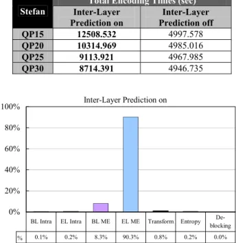
In this section, we first analyze the coding efficiency of inter-layer prediction. As shown in Fig. 1, inter-layer prediction can substantially improve the rate-distortion performance compared with that without using inter-layer prediction. However, inter-layer prediction will also incur excessive encoding time as Table 1 shows. We next analyze

(2)

Inter-Layer Prediction on 0% 20% 40% 60% 80% 100% % 0.1% 0.2% 8.3% 90.3% 0.8% 0.2% 0.0% BL Intra EL Intra BL ME EL ME Transform Entropy

De-blocking

Fig. 2. Computation complexity of each coding tool in H.264/ SVC. Stefan 27 29 31 33 35 37 39 41 43 100 600 1100 1600 2100 2600 3100 3600 4100 Bitrate(Kbps) PSNR (d B ) Inter-Layer Prediction on Inter-Layer Prediction off

Fig. 1. Coding performance comparison between H.264/SVC with and without inter-layer prediction.

Table 1. Encoding time comparison between H.264/SVC with and without inter-layer prediction

Total Encoding Times (sec) Stefan Inter-Layer Prediction on Inter-Layer Prediction off QP15 12508.532 4997.578 QP20 10314.969 4985.016 QP25 9113.921 4967.985 QP30 8714.391 4946.735

Table 2. The contribution of each motion vector predictor

Stefan_ELMVPUse _BLMVPUse Forema_n _ELMVPUse _BLMVPUse QP 15 73.9% 26.1% QP 15 76.9% 23.1%

QP 20 72.3% 27.7% QP 20 81.3% 18.7%

QP 25 73.8% 26.2% QP 25 87.0% 13.0%

QP 30 78.4% 21.6% QP 30 91.9% 8.1%

QP 35 85.8% 14.2% QP 35 95.7% 4.3%

the computation complexity of each coding tool when the inter-layer prediction is enabled. The results are shown in Fig. 2. Similar to H.264/AVC single layer coding, we can observe that motion estimation also occupies most of the encoding time in H.264/SVC. In particular, the encoding time of the enhancement layer motion estimation is about 10 times of the base layer. Hence, encoding with inter-layer prediction is necessary in general and the speed-up of enhancement layer motion estimation is also required. The reason why the inter-layer prediction leads to extra computational complexity is described as follows.

Enhancement layer motion estimation in B frames has to execute three temporal direction predictions, i.e. forward,

backward, and bi-prediction, with median motion vector predictor (ELMVP) and then chooses the best one as the final prediction. When inter-layer prediction is utilized, inter-layer motion prediction will additionally execute the motion estimation with another motion vector predictor. This additional predictor is up-scaled from the best motion vector of the corresponding block in the base layer (BLMVP) if the base layer information in each temporal direction is available. Therefore, enhancement layer will additionally execute the procedure of motion estimation. Our objective is to determine whether to perform motion estimation based on the base layer motion vector and which temporal direction will be chosen in advance.

3. PROPOSED FAST INTER-LAYER MOTION ESTIMATION ALGORITHM

Our proposed algorithm contains two major parts: selective reference layer motion vector predictor and temporal direction decision of small block mode motion estimation. In the remainder of this section we will introduce both parts respectively.

3.1. Selective Reference Layer Motion Vector Predictor In H.264/SVC, enhancement layer executes the motion estimation with both ELMVP and BLMVP, and then chooses the best one. Table 2 shows the ratio of choosing each motion vector predictor as the final motion vector predictor when we utilize both ELMVP and BLMVP. The results indicate that the contribution of BLMVP is much smaller than that of ELMVP. Therefore, our algorithm focuses on when we have to execute motion estimation with BLMVP.

We first measure the distance between ELMVP and BLMVP as shown in Table 3, and the distance between motion vector searched by ELMVP (ELMV) and that searched by BLMVP (BLMV) as shown in Table 4. MVPd and MVd are calculated as (1) and (2) respectively.

MVPd= ELMVPx BLMVPx− + ELMVPy BLMVPy− (1)

MVd= ELMVx BLMVx− + ELMVy BLMVy− (2) According to Table 3, we can find that the distance between BLMVP and ELMVP is most probably to be less

(3)

Table 3. The distance between ELMVP and BLMVP

QP 15 Stefan Foreman Akiyo Mobile 0≦MVPd≦2 79.3% 77.7% 93.8% 90.7%

2＜MVPd 20.7% 22.3% 6.2% 9.3%

2＜MVPd 21.3% 22.4% 6.2% 9.8%

2＜MVPd 22.8% 21.3% 6.1% 9.6%

2＜MVPd 22.6% 19.4% 6.0% 9.2%

Table 4.The distance between ELMV and BLMV

QP 15 Stefan Foreman Akiyo Mobile

MVd=0 82.6% 78.2% 92.6% 92.5%

0＜MVd≦1 5.4% 10.9% 1.9% 2.0%

1＜MVd 12.0% 10.8% 5.5% 5.5%

MVd=0 78.7% 70.8% 91.8% 90.5%

0＜MVd≦1 8.4% 15.9% 2.5% 3.6%

1＜MVd 12.9% 13.3% 5.7% 5.8%

MVd=0 73.0% 63.8% 91.6% 87.7%

0＜MVd≦1 11.8% 19.4% 2.6% 6.1%

1＜MVd 15.2% 16.8% 5.8% 6.2%

MVd=0 67.3% 60.9% 91.8% 83.2%

0＜MVd≦1 15.8% 19.7% 2.2% 10.3%

1＜MVd 17.0% 19.4% 5.9% 6.5%

Fig. 4. Notations definition.

Fig. 5. Case 2:PreMVD ELMVD≤ .

Cost_E =D_E+λ_motionR_E (3)

CostB =DB+λmotionRB (4)

Where D is the SAD (sum of absolute difference) between the current block and the reference block, R denotes the bits cost for encoding the MVD (motion vector difference), and λ is the Lagrange multiplier. The suffixes E and B denote the ELMVP and BLMVP respectively.

Next we use the statistics mentioned above to discuss three cases and propose the criterion for whether to employ BLMVP. For the convenience, we define notations as shown in Fig. 4, where ELMVD (BLMVD) is the difference between ELMVP (BLMVP) and ELMV (BLMV), PreMVD is the difference between BLMVP and ELMV.

Fig. 3. The distribution of BLMVP.

♦ Case1: ELMVP = BLMVP

When BLMVP is the same as ELMVP, CostB is obviously the same as CostE. Therefore, we get the first decision trivially.

We employ the BLMVP only when BLMVP ≠ELMVP.

than or equal to 2. Figure 3 shows this condition, the blue region is the region that BLMVP most probably is located in. According to Table 4, we can observe that no matter we execute motion estimation with ELMVP or BLMVP, the best points searched by both motion vector predictors will most probably be the same. Besides, there is about 90% probability that the distance between ELMV and BLMV is less than or equal to 1.

♦ Case2: PreMVD ELMVD≤

This case is shown in Fig. 5, the orange region is the region conforming to this case. Because ELMV is also a candidate of the search point for BLMVP, in this case, DB is the same as DE, and RB must be less than or equal to RE. In other

words, if PreMVD ELMVD≤ , CostB must be less than or

equal to CostE, and it is worth to employ BLMVP.

Combining this condition with the first one, we can get the new decision.

Similar to H.264/AVC, motion estimation in H.264/SVC is performed by minimizing the rate-distortion cost function. We define the cost functions for ELMVP and

BLMVP as the following equations. _{We employ the BLMVP only when BLMVP}_≠ _{ELMVP and}

(4)

Fig. 6. Case 3:PreMVD > ELMVD.

(a) ELMVD = 1 (b) ELMVD = 2

Fig. 7. Illustration of adaptive search range of BLMVP.

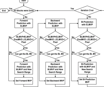
Fig. 8. Flow chart of selective reference layer motion vector predictor.

♦ Case3: PreMVD > ELMVD

Although CostB will be less than or equal to CostE in case 2, it still has a chance that CostB to be less than CostE when PreMVD is larger than ELMVD. Therefore, we extend 1 pixel to the prior condition, and we infer that it should be enough. As shown in Fig. 6, the light orange region is the extended region. When BLMVP is located in the light orange region, BLMVP may choose the point closer to it as the best point rather than ELMV. At this time, it still has a

chance that CostB to be less than CostE. Finally, we

conclude all the conditions to get the final decision.

We employ the BLMVP only when BLMVP ≠ ELMVP and Pixel.

PreMVD ELMVD + 1≤

Table 5 shows the hit rate between the original JSVM full search and our proposed decision. Although the hit rate becomes lower when QP becomes larger, the effect on the coding efficiency is very small. Because the probability that BLMVP to be chosen as the final motion vector predictor also becomes lower (can be observed from Table 2).

Fig. 8 is the proposed flow chart of selective reference layer motion vector predictor algorithm.

3.2. Temporal Direction Decision of Small Block Mode Motion Estimation

Table 5. The hit rate of our proposed decision

Stefan Foreman Akiyo Mobile

QP 15 89.5% 92.3% 98.9% 98.3%

QP 20 87.7% 90.0% 97.4% 97.8%

QP 25 83.8% 84.5% 95.5% 97.0%

QP 30 80.7% 77.0% 91.7% 96.2%

QP 35 76.3% 65.9% 84.9% 94.2%

In H.264/SVC, 8x8 block size is a unit of setting the temporal direction. There must be a high correlation between Mode8x8 and other modes. According to the results of our statistics, the temporal direction of the modes smaller than Mode8x8 has an over 85% opportunity to be the same as Mode8x8. Therefore, we propose to only execute the same temporal direction motion estimation of Mode8x8 for the modes smaller than Mode8x8.

We have been able to efficiently employ the BLMVP, and we further want to save the search points of BLMVP. According to Table 4, since the best points searched by ELMVP and BLMVP are very close, we can narrow the search range of BLMVP. Our proposed adaptive search range of BLMVP is set to ELMVD as shown in Fig. 7. At this time, RB must be less than or equal to RE, and the CostB

may be less than CostE. However, ELMVD may be in a

sub-pixel unit, so we extend the adaptive search to the smallest integer larger than ELMVD, i.e.

4. SIMULATION RESULTS

Our scheme is implemented on JSVM9.12. The test platform is Intel Core 2 Quad 2.40GHz CPU, 2G RAM with Windows XP professional operating system. The simulation setting is shown in Table 6. In our experiments, six standard test sequences including Akiyo, Crew, Foreman, Harbour, Mobile and Stefan have been tested. The performance assessments in our experiments include the time saving, the ELMVD .

(5)

Table 6. Simulation setting

JSVM Version 9.12

Layer Base Layer Enhancement Layer

Resolution QCIF CIF

FrameRate 30 30 QP 15, 20, 25, 30, 35 SearchRange 32 FramesEncoded 300 GOP 16 InterLayerPrediction on SequenceType IBB…PBB…P

Table 7. Simulation results with QP=15 and QP=35

QP15 △PSNR(dB) △bitrate TimeSave akiyo -0.0002 0.10% 64.0% crew -0.0104 0.39% 58.1% foreman -0.0079 0.90% 60.6% harbour -0.0017 0.29% 67.4% mobile -0.0105 0.31% 65.8% stefan -0.0123 1.05% 63.3% QP35 △PSNR(dB) △bitrate TimeSave akiyo 0.0048 0.13% 63.6% crew -0.0136 -0.24% 59.5% foreman -0.0028 0.19% 61.0% harbour -0.0019 0.02% 63.6% mobile -0.0165 0.47% 61.4% stefan -0.0476 0.52% 59.5%

difference of Y-PSNR (ΔPSNR) and the difference of bit

rate (Δbitate). They are defined as (5), (6), and (7). 100% JSVM proposed JSVM T T TimeSave T − = × (5) proposed JSVM PSNR PSNR PSNR Δ = − (6)

[3] Coding of audio-visual objects-Part 2: Visual, ISO/IEC

14492-2 (MPEG-4 Visual), ISO/IEC JTC 1, Version 1: Apr. 1999, Version 2: Feb. 2000, Version 3: May 2004.

100% proposed JSVM JSVM bitrate bitrate bitrate bitrate − Δ = × (7)

[4] H. Schwarz, D. Marpe, and T. Weigand, “Overview of the Scalable Video Coding Extension of the H.264/AVC Standard,” IEEE Trans. Circuits Syst. Video Tech., vol. 17, no. 9, pp. 1103-1120, Sep. 2007.

The experiment results with QP=15 and QP=35 are given in Table 7. The proposed algorithm can save 58%-67% total encoding time compared with JSVM9.12 with less than

0.0476dB video quality degradation. [5] C. A. Segall and G. J. Sullivan, “Spatial Scalability Within the _{H.264/AVC Scalable Video Coding Extension,”}_{IEEE Trans.}

Circuits Syst. Video Tech., vol. 17, no. 9, pp. 1121-1135, Sep.

2007.

5. CONCLUSION

[6] H. Li and Z. G. Li, “Fast Mode Decision Algorithm for Inter-frame Coding in Fully Scalable Video Coding,” IEEE Trans.

Circuits Syst. Video Tech., vol. 16, no. 7, pp. 889-895, Jul.

2006.

In this paper, we propose a fast inter-layer motion estimation algorithm for H.264/SVC. We utilize the relation between two motion vector predictors of base layer and enhancement layer. The correlation of temporal prediction direction between all the modes is also used to reduce the number of searches. The algorithm can determine whether to perform motion estimation with base layer motion vector predictor (BLMVP) and which temporal direction will be chosen in advance. The algorithm achieves high encoding time saving while maintains very good rate-distortion performance. Besides, the proposed algorithm can be easily integrated with common fast motion search algorithms such as diamond search and combined with existing fast mode decision algorithms to further reduce the encoding time.

[7] H. Li, Z. G. Li, C. Wen, and L. P. Chau, “Fast Mode Decision for Spatial Scalable Video Coding,” IEEE International

Symposium on Circuits and Systems, May 2006, pp. 3005-3008.

[8] H. Li, Z. G. Li, and C. Wen, “Fast Mode Decision for Coarse Grain SNR Scalable Video Coding,” IEEE International

Conference on Acoustics, Speech and Signal Processing, May

2006, vol. 2, pp. 545-548.

[9] S. Lim, J. Yang, and B. Jeon, “Fast coding mode decision for scalable video coding,” International Conference on Advanced

Communication Technology (ICACT), Feb. 2008, vol.3,

pp.1897-1900.

[10] S. T. Kim, K. R. Konda, and C. S. Cho, “Fast Mode Decision Algorithm for Spatial and SNR and Scalable Video Coding,”

IEEE International Symposium on Circuits and Systems (ISCAS

2009), May 2009, pp. 872-875.

6. REFERENCES

[11] C. S. Park, S. J. Baek, M. S. Yoon, H. K. Kim, and S. J. Ko, “Selective Inter-layer Residual Prediction for SVC-based Video Streaming,” IEEE Trans. Consum. Electron., vol. 55, no. 1, pp. 235-239, Feb. 2009.

[1] Generic Coding of Moving Pictures and Associated Audio

Information-Part 2: Video, ITU-T Rec. H.262 and ISO/IEC

13818-2 (MPEG-2 Video), ITU-T and ISO/IEC JTC 1, Nov. 1994.

[2] Video Coding for Low Bit Rate communication, ITU-T Rec.

H.263, ITU-T, Version 1: Nov. 1995, Version 2: Jan. 1998, Version 3: Nov. 2000.