Do consumers gamble to convexify?

Do consumers gamble to convexify?

IFS Working Paper 07/11

Thomas F. Crossley Hamish Low

Do Consumers Gamble to Convexify?

Thomas F. Crossley

University of Cambridge and Institute for Fiscal Studies (IFS) Hamish Low

University of Cambridge and IFS Sarah Smith

University of Bristol and IFS May 2011∗

Abstract

The combination of credit constraints and indivisible consumption goods may induce some risk-averse individuals to play lotteries to have a chance of crossing a purchasing threshold. One implication of this is that income effects for individuals who choose to play lotteries are likely to be larger than for the general population. Using UK data on lottery wins, other windfalls and durable good purchases, we show that lottery players display higher income effects than non-players but only amongst those likely to be credit constrained. This is consistent with credit constrained, risk-averse agents gambling to convexify their budget set.

JEL classifications: D12, E21, D81, L83

Keywords: Gambling, Lotteries, Consumption, Durables

* This work was supported in part by the ESRC-funded Centre for Microeconomic Analysis of Public Policy at the Institute for Fiscal Studies (grant number RES-544-28-5001.) For helpful comments and suggestions we thank Sule Alan, Helen Simpson and seminar participants at Royal Holloway University of London, McMaster University, Leicester University and the Lincoln College Applied Microeconometrics Conference at the University of Oxford. All errors are our own.

Correspondence: Hamish Low, Faculty of Economics University of Cambridge Austin Robinson Building, Sidgwick Avenue, CAMBRIDGE CB3 9DD, Email: [email protected] Phone: +44 1223 335221

“On Friday September 4th 1994, the freezer belonging to Gloria and Steve Kanoy of Weere’s Cove suddenly and mysteriously broke down. Distraught, the couple set off the next day in search of a new one. Stopping for gas at Lake Raceway, 607 Main Avenue, they decided to buy a Lotto ticket…”

Virginia Lottery winner awareness campaign, quoted in Clotfelter and Cook (1990)

1.

Introduction

Why do risk-averse individuals gamble? One explanation, first developed by Ng (1965), is that discreteness in spending or in labour supply opportunities can induce local non-concavities in the value functions of averse agents. This generates local risk-loving behaviour and makes it rational for them to gamble in order to have a chance of crossing the threshold required to finance a lumpy purchase, such as the freezer in the quote above. Bailey et al (1980) argued that access to credit markets made such gambling irrational, but Hartley and Farrell (2002) showed theoretically that rational gambling might still occur where borrowing and lending rates differ, where capital market imperfections exist, or if individuals' time preference rates differ from interest rates. Whilst this may be true in theory, there is a lack of empirical research that addresses whether consumers “gamble to convexify” in practice. This is the focus of this paper, using data from the UK.

This is important for three key reasons. First, and most obviously, it helps to understand (at least part of) the demand for gambling and lotteries. In the UK, this includes the National Lottery, the largest state-run lottery in the world with average weekly sales of £36 million, and also premium bonds, a government bond which pays a return in the form of an entry to a prize draw, which are held by an estimated 40 per cent of households. Tufano (2008) and Kearney et al (2010) have emphasized the entertainment aspect of prize-linked savings products in explaining their potential attraction. The desire for convexification provides another rationalization for that demand despite individuals being risk averse. In many developing countries, there is also the interesting case of rotating savings and credit associations (ROSCAs), discussed by Besley et al (1993). These are a micro-finance initiative in which groups of individuals make regular contributions to a fund, the total amount of which is allocated to one

member each cycle via a lottery. Handa and Kirton (1999) provide evidence from Jamaica that people use their allocation from the ROSCA to buy durable goods.

Second, a number of authors, notably Imbens et al. (2001), have used lotteries to estimate income effects in labour supply and consumption demands. Income effects are central to policy evaluation, but standard estimation procedures suffer from a lack of plausibly exogenous variation in income. Imbens et al. exploit the fact that lottery winnings provide random variation in income among lottery players. Of course, as Imbens et al. recognise, those who play the lottery may differ from those who do not. The key point we make is that the “convexification” hypothesis provides a compelling economic rationale for expecting this to be the case. In particular, the desire to convexify generates a demand for lotteries among precisely those individuals who are close to the threshold of a discrete decision (for example, purchasing a durable or retiring) and who therefore will display large income effects. The resulting threat to the external validity of the estimates is analogous to randomization bias (Heckman and Smith, 1995) in

randomized trials: those who participate in the random allocation of treatment are

systematically different from those who do not. An empirical strategy of measuring income effects based on lottery winnings may thus overestimate the average response to a more broadly distributed windfall. Interestingly, Imbens et al. report that lottery winnings appear to have larger effects on discrete margins, such as retirement.

The third reason the convexification hypothesis is important arises because non-convexities due to the discreteness of choices pose a major technical challenge to researchers trying to model those choices structurally with dynamic programming models. One way to overcome this problem has been to assume that individuals facing such non-convexities play wealth lotteries (Rogerson, 1988; Lentz and Traneas, 2004). It is important to establish whether this is simply a technical convenience or whether this captures the way that individuals actually behave when faced with non-convexities.

To highlight the mechanisms at work, we first develop a simple model where consumers choose whether or not to buy a lottery ticket, and then after the outcome of the lottery is known, whether or not to buy an indivisible good. The only consumers who buy the lottery ticket are those who are close to the threshold of being able to buy the indivisible good. A lottery win then enables the purchase of the indivisible good.

To look for evidence that consumers gamble to convexify we use data from the British Household Panel Survey. Our empirical strategy is effectively a “difference-in-difference” design, contrasting estimated income effects for lottery windfalls with those for other windfalls (specifically inheritances) among those that are credit constrained with those that are not. We use the group who are not credit constrained to control for more general differences in responses by windfall type – including the degree to which alternative windfalls are anticipated, unobservable characteristics of individuals who gamble and inherit or psychological feelings attached to different sources of windfall. We also use data on financial expectations to examine directly whether inheritances are more anticipated than lottery winds. There is no evidence in these data that this is the case.

Our main result is that, among individuals who are credit constrained, purchases of consumer durable goods are more responsive to a lottery win than to receipt of other windfall income: individuals whose income increases by gambling and winning are more likely to be buying durables. This is not the case among individuals who are not credit constrained. This finding is exactly what we would expect if credit-constrained consumers gamble to convexify. As a further test, we examine the effects of non-lottery windfalls on individuals who can be inferred to have played the lottery but not had large winnings. For the subset of these individuals who are credit constrained, purchases of consumer durable goods are more responsive to non-lottery windfall income than purchases by non-players: those who play the lottery exhibit larger income effects than those that do not play. Thus, consistent with our hypothesis, it is not the source of the money (lottery versus other windfall) that matters, but rather that lottery players that are different from non-players.

We are not claiming that the desire to convexify explains all gambling, but our results suggest that it is a reason why some people gamble, and that therefore the use of lottery winnings as an instrument for identifying income effects will have very poor external validity: this instrument identifies the income effect for a group with very large income effects.

An outline of the rest of the paper is as follows. In the next section we develop the theoretical framework that guides our analysis. In Section 3 we examine the implications of the model for the resulting income effects if lotteries are endogenously chosen. Section

4 describes our data and empirical framework. Section 5 presents our main results, and Section 6 concludes.

2.

A Model of Gambling to Finance Indivisible Purchases

Our model is a one period model with two stages.1 At the start of the period (in

the first stage), agents have cash on hand x₁. They first make a decision about whether or

not to buy at most one lottery ticket: l∈

{ }

0,1 , where the price of the lottery ticket is 1.

They then discover whether or not they have won. The lottery ticket is actuarially fair:2

an agent holding a ticket wins 1qwith probability q, so that net winnings are

(

1−q

)

q

with probability qand −1 with probability 1−q. Net winnings augment an agent’s

cash-on-hand. Thus, x₂ =x₁if a ticket is not purchased, but if a ticket is purchased, disposable

cash-on-hand will be x₂ = + −x₁

(

1 q q

)

with probability qand x₂ = −x₁ 1 with

probability1−q.

After lottery winnings are revealed, individuals decide, in the second stage, how to allocate their spending between a divisible consumption good and an indivisible

consumption good. Agents can buy at most one unit of the indivisible good (d∈0,1) at

pricep. In our empirical work, the indivisible goods will be consumer durables. Without

borrowing or saving, consumption of the divisible good is justx₂−dp. Individuals

maximize utility, which depends on the consumption of divisible and indivisible goods:

2 2

( , ) ( )

v x −dp d =u x −dp +ηd; ηis a preference parameter. We assume that u'

( )

⋅ >0,

( )

'' 0

u ⋅ < and u(0)+ <η u p( ), where this last condition specifies that the individual will

not buy the indivisible good if this implies 0 consumption of the divisible good. 3

1 _{This means we can abstract from borrowing and saving. As discussed later, the ability to borrow and save} is likely to reduce the need to gamble to convexify. We exploit this difference in our estimation procedure, but we abstract from this in our model to make the motive for gambling transparent.

2 _{We could introduce a penalty for gambling and make the gamble actuarially unfair, but this would simply} act to offset the motive to gamble caused by the non-convexity.

3 _{The additive separability assumed here is not necessary. It is however necessary to restrict the degree of} substitutability between durable and non-durable consumption.

We solve this simple model by backward induction. Define

1

2 ( )2 ( 2 )

d

V = x =u x −p +η and V₂d=0( )x₂ =u x( )₂ . The indivisible good is purchased if and

only if 1 0

2 ( )2 2 ( )2

d d

V = x ≥V = x , ie. u x( ₂−p)+ ≥η u x( )₂ .

Result 1 (single-crossing): There is a unique x₂* such that the indivisible good is purchased if and only if x₂ ≥x₂* . x*₂ is implicitly defined by u x( ₂*−p)+ =η u x( )*₂ .

Proof: Uniqueness follows from the fact that

( )

( )

0 1 2 2 2 2 2 2 2 2 2 '( ) '( ) d d V x V x u x u x p x x x = = ∂ ∂ = < = − ∀ ∂ ∂ ₍₁₎

which in turns follows from the concavity of u

( )

⋅ .

This difference in the derivative of the conditional value functions implies that the unconditional value function is non-concave because the derivative changes discretely at the point where the two value functions cross. This is illustrated in Figure 1.

[Figure 1, Single Crossing, About Here]

Turning to the first stage, in which the decision to gamble is taken, let 1

1 ( )1

l

V = x be the

value of purchasing the lottery ticket and 0

1 ( )1

l

V = x the value of not gambling. A lottery

ticket is purchased if and only if 1 0

1 ( )1 1 ( ) 01 l l E V⎡_⎣ = x ⎤ −_⎦ V = x ≥ . Note that: 0 1 1 1 1 * 1 1 2 * 1 1 2 ( ) max[ ( ) ), ( ,0)] ( ) if ( ) if l V x u x p u x u x p x x u x x x η η = _{= − +} ⎧ − + ≥ ⎪ = ⎨ < ⎪⎩ ₍₂₎ and

(

)

(

)

(

)

(

)

[

]

1 1 1 1 1 1 1 ( ) max 1 , ( 1 ) + 1 max ( 1) , ( 1) l E V x q u x p q q u x q q q u x p u x η η = _{⎡ ⎤} ⎡ ⎤ = − + − + + − ⎣ ⎦ ⎣ ⎦ − − − + − (3)

Result 2: Lottery tickets are not purchased outside the interval x₂* 1 q,x₂* 1 q

⎡ ₋ − ₊ ⎤

⎢ ⎥

⎣ ⎦.

The intuition behind this result is straightforward. If *

1 2 1

x >x + _{the agent}

purchases the indivisible good regardless of the outcome of the lottery. Thus only 1

2

d

V = is

relevant, and the concavity of 1

2

d

V = (which is inherited from the concavity of u

( )

⋅ )

ensures that the agent does not gamble. If *

(

)

1 2 1

x <x − −q q the agent does not purchase

the indivisible good regardless of the outcome of the lottery. Thus only 0

2

d

V = is relevant,

and the concavity of 0

2

d

V = (which is inherited from the concavity ofu

( )

⋅ ) ensures that the

agent does not gamble.The bounds, *

(

)

2 1

x − −q q and x*₂+1 are illustrated in Figure 2.

[Figure 2, Regions]

Corollary 1: A lottery winner always purchases the indivisible good.

Proof: Since lottery tickets are never bought if x₁<x*₂− −

(

1 q q

)

, a lottery winner (with

net winnings

(

1−q

)

q) always has x₂≥x*₂.

Corollary 2: A lottery player that does not win does not purchase the indivisible good.

Proof: Since lottery tickets are never bought if x₁≥x*₂+1, any unsuccessful lottery

player (with net winnings −1) always has *

2 2

x <x .

Result 3: There exists a compact region, x1∈ ⎣⎡x x1, 1⎤⎦, which contains * 2

x

(

x1<x*2 <x1

)

,

in which the agent will purchase a lottery ticket.

Proof: See appendix.

From Result 2, we know that x₂*− −

(

1 q

)

q≤x₁<x₁≤x₂*+1. Within these bounds,

the size of the regionx₁∈ ⎣⎡x x₁, ₁⎤_⎦ depends on parameter values (η,qand the curvature of

of u

( )

⋅ ).

Together, Corollaries 1 and 2, and Result 3 imply that the state space (of cash on

hand) can be divided into three regions. A region x₁≤x₁ in which the agent does not buy

a lottery ticket and does not buy the indivisible good; a region x₁< ≤x₁ x₁in which the

a regionx₁ >x_{1 in which the agent does not buy the lottery ticket but does buy the}

indivisible good. This is illustrated in Figure 2.

What this simple model illustrates is that lottery players are very likely to be close to the margin of a discrete decision. This implication that lottery players are gambling to convexify is tested in section 4 by looking at the income effects of gamblers and non-gamblers. In the next section we show the implications of our model for using lotteries to estimate income effects. Estimated income effects form the basis of subsequent empirical tests.

3

Implications for Estimating Income Effects

In this section, we show that the estimated income effect (i.e. the effect of income on the purchase of an indivisible good) associated with an endogenously chosen lottery will be a biased estimate of the population average income effect. To show this, we consider the follow thought experiment, which we refer to as a randomly assigned lottery:

a random fraction (λ) of the population is compelled to buy the lottery ticket, and no

other tickets are available. This thought experiment holds the number of tickets constant, but removes the element of choice from gambling. This leads to a measure of the income effect from lottery winnings when the lottery ticket purchase is random, and thus to a population average income effect.

We consider two cases, corresponding to two different data structures. In the first case, as in Imbens et al. (2001), income effects are estimated by comparing lottery winners and lottery losers (i.e. people who play the lottery, but lose). In the second case, the comparison is between winners and non-winners; the latter includes both losers and non-players. We show that in both cases the extra spending by winners is a biased estimate of the population average income effect (which would be the income effect arising from a truly exogenous windfall.)

3.1. Comparing Winners and Losers.   

First, consider the comparison between lottery winners and lottery losers. In the model developed above, an agent always buys the indivisible good if they are a lottery

probability that a lottery winner purchases the indivisible good is one:

( 1| , ) 1

Prob d = winner choice = . We condition the probability on “choice” to indicate that

playing the lottery was a decision taken by the individual. These probabilities are summarized in Table 1.

In the case of the randomly allocated lottery on the other hand, lottery winners

who have net winnings of

(

1−q

)

q giving x₂= + −x₁

(

1 q q

)

, will purchase the

indivisible good if *

(

)

1 2 1 x ≥x − −q q. Thus

(

)

(

*

)

2 ( 1| , ) 1 1

Prob d = winner rand = −F x − −q q .

Thus winners from the chosen lottery are more likely to purchase the indivisible good than winners of the randomly allocated lottery:

0 1 ) , | 1 ( Pr ) , | 1 ( Pr * 2 ⎟⎟≥ ⎠ ⎞ ⎜⎜ ⎝ ⎛ − − = = − = q q x F rand winner d ob choice winner d ob (4)

The intuition behind this result is straightforward. In the case of the randomly allocated

lottery, some winners will come from below the lower threshold _⎟⎟

⎠ ⎞ ⎜⎜ ⎝ ⎛ − − q q

x*₂ 1 and will not

have enough cash on hand to buy the divisible good even if they win. This difference

tends to zero as q becomes increasingly small: if there is a lottery prize that is very large

but with a very small probability of winning, it is in the interest of everyone with

cash-on-hand below *

2

x to gamble to convexify, and all winners will chose to buy the

indivisible good, whether the lottery ticket was chosen or randomly allocated.

For those that chose to play, but lost, the probability that the non-winner

purchases the indivisible good is zero: Prob d( =1|lost choice, ) 0= . By comparison,

among the losers in the randomly allocated lottery are some people with cash on hand

above the upper threshold

(

* 1

)

2 +

x who will have enough cash on hand to purchase the

divisible good even if they lose, i.e. Pr ( 1| , ) 1

(

* 1

)

.

2 + − = = lost rand F x d ob The

probability of purchase is therefore lower among losers of the endogenous lottery than among losers of the randomly allocated lottery:

(

1

)

1 0 ) , | 1 ( Pr ) , | 1 ( Pr * 2 + − ≤ = = −

= loser choice ob d loser rand F x d

Putting together the differences in purchase probabilities between winners and the

difference in purchase probabilities between losers, it is clear that the income effect in the case of the endogenous lottery suffers from upward bias compared to income effect from the randomly allocated lottery. The latter is an unbiased estimate of the population

average income effect. An expression for the bias is given in the final row of the second d

column of Table 1. The size of the bias becomes smaller as the range in which tickets are bought becomes larger.

3.2. Comparing Winners and Non-winners   

Non-winners comprise both non-players and losers. In the case of the endogenous

lottery, those who choose not to play are those with x₁<x₁ or x₁>x₁ while losers are

the fraction 1−q of lottery players, who all have x1< ≤x1 x1. Of these non-winners, only

agents with cash on hand x₁ >x₁ buy the indivisible good. Let λdenote the faction of

lottery players: λ=F x

( )

1 −F x

( )

1 , where F

( )

⋅ is the cumulative distribution of cash on

hand (x1) in the population. Thus

( )

1

( )

1

1 1

( 1| , )

1 ( ) 1

F x F x Prob d non winner choice

Prob winner qλ

− −

= − = =

− − ₍₆₎

The effect of winning the lottery (relative to non-winners) on the probability of indivisible good purchase is therefore the difference:

(

)

(

)

( )

( )

1 1 1 1 , 1 , 1 1 1 F x Prob d winner choice Prob d non winner choice

q F x q q λ λ λ − = − = − = − − − = − ₍₇₎

In the randomly assigned lottery, non-winners comprise those that were randomly allocated a ticket but did not win, and those that were not allocated a ticket. The former

are fraction (1−q)λof the population, have net winnings of −1and purchase the durable

if *

1 2 1

purchase the durable if *

1 2

x ≥x . The overall fraction of the population that are

non-winners is, as before, (1−q)λ+ −(1 λ) 1= −qλ. Thus the fraction of non-winners who

purchase the durable is:

(

)

(

)

(

*

)

(

( )

*

)

2 2 ( 1, , ) ( 1| , ) , (1 ) 1 1 (1 ) 1 1

Prob d non winner rand Prob d non winner rand

Prob non winner rand

q F x F x q λ λ λ = − = − = − − − + + − − = − ₍₈₎

This can be interpreted more easily if we approximate *

2

( 1)

F x + by F x( )*₂ : this is a good

approximation if the price of the lottery ticket, 1, is small compared to typical cash-on-hand. The probability then becomes:

( )

(

*

)

(

)

2 1 1 ( 1| , ) 1 F x q Prob d non winner rand

q λ λ − − = − = − ₍₉₎

The denominator is the fraction of the population who are not winners. The first part of

the numerator,

( )

*

2

1−F x , is the fraction of all individuals whose cash-on-hand means

they would purchase the durable regardless of the lottery. Some of these individuals will be winners when the lottery tickets are randomly allocated and so this fraction is multiplied by the fraction of the population that are not winners.

By contrast, when the purchase of the lottery ticket was a choice, none of those individuals who would purchase regardless of the lottery choose to buy lottery tickets and so they are all winners, and the probability of purchasing the durable among non-winners is given by equation (6).

To aid interpretation of the difference between equation (9) and (6), approximate

1

( )

F x byF x( )₂* (recall from Results 2 and 3 that x*₂ <x₁≤x₂*+1). This gives a difference

in the probability of purchase among non-winners from the chosen and random lotteries of:

( )

(

*

)

2 1 ( 1| , ) ( 1| , ) 0 1 q F x Prob d non winner choice Prob d non winner rand

q λ λ − = − − = − = ≥ − (10)

The probability of purchasing the durable among the non-winners from the chosen lottery is higher. This arises from a subtle composition effect because the group of non-winners comprises two sets of individuals: those who did not have a ticket and those that had a losing ticket. Some of those who were non-winners by choice (ie chose not to have a ticket because they would have purchased the durable anyway) became random lottery winners, and this reduces the number of purchasers of the durable among those who were not winners.

When we compare winners and non-winners of the lottery, the probability of purchasing the durable is higher among both winners and losers when the lottery ticket is chosen. This implies that the effect of winning the (chosen) lottery on durable purchases may be greater or smaller than the effect of winning on purchases when the allocation is random. The net effect is given by:

( )

* * * 2 2 2 1 1 1 1 q q F x q F x F x q q q λ λ ⎛ ⎛ ⎞⎞ ⎛ ₋ − ⎞_{− − −} ⎛ ₋ − ⎞ ⎜ ⎜ ⎟⎟ ⎜ ⎟ _⎜ ⎜ ⎟ _⎟ ⎝ ⎠ ⎝ ⎝ ⎝ ⎠⎠⎠ − ₍₁₁₎

When the probability of winning, q, is small and the prize large, the first term on the

numerator is close to zero and the negative composition effect might dominate. On the

other hand, as q gets larger, the second term tends to λqand the net effect is positive: the

effect of the winners of the chosen lottery being more likely to purchase the durable dominates.

These two offsetting differences can be highlighted by calculating numerically the size of the effects in our simple model, at particular parameter values. We assume log utility for consumption, and consider a high and low value for the utility of the durable

(η). Figure 3 shows the difference in the probability of purchase between the chosen and

random lotteries. For these parameters, estimates of the effect of a windfall on the purchase of the durable from lotteries will overestimate the effect of a random windfall

[Figure 3, Simulation, About Here] 3.3. Discussion

The aim of this model was to highlight the differing income effects arising from different sorts of windfall gain. In particular, the effect of a windfall on indivisible purchases is likely to be larger if the windfall arises from a lottery that the household has chosen to participate in. This arises because the indivisibility means households have an incentive to gamble to convexify. However, the strength of this incentive will be diminished if capital markets are well functioning, and so agents can borrow or save, because this allows the path of non-durable consumption to be unaffected by the timing of indivisible purchases (Bailey et al., 1980; Hartley and Farrell, 2002). The need to gamble to convexify is also diminished if there are multiple indivisible goods so that the indivisibility is less “lumpy”, or if there are uninsurable income shocks which provide some convexification. This means that the importance of the convexification hypothesis is an empirical question, and in the remainder of this paper we assemble empirical evidence on this question. While data on lottery players cleanly identifies the income effect among players, this data structure is incapable of shedding light on the convexification hypothesis that the income effects among lottery players are different from those of nonplayers. Thus we turn to a general population survey. We can however also use our general survey to approximate the data set focused only on lottery players used by Imbens et al (2001) (see the discussion of the small winnings test in Sections 4 and 5).

4. Empirical Framework and Data

4.1. Empirical framework

We adopt a reduced form empirical approach but one that is directly motivated by the discussion in the previous section. There we showed that endogenous gambling results in income effects that are biased compared to those based on an exogenous windfall. Our main empirical strategy is to examine a difference-in-difference in income effects. In particular, we compare the effect of windfalls on purchases of indivisible

goods between lottery winners4 and those who receive another type of windfall – namely an inheritance, and we compare these differences between those who are likely to be credit constrained and those who are not.

In the context of the model above, inheritances are intended to approximate the

randomly allocated lottery. The assumption is not that inheritances are random across the

population, but that they are exogenous with respect to the distance between cash on hand

(x₁) and the critical value (x*₂), conditional on controls and individual fixed effects. Note

that the critical value will vary in the population and over time for a given individual according to tastes and needs.

Our empirical work focuses on durable goods, which are inherently indivisible; our prediction is that durable purchases will respond differently to a lottery win than to an inheritance because the people who receive lottery winnings are on average closer to the threshold of a discrete purchase. This is the convexification hypothesis and it is a selection effect: different windfalls are received by different people.

If we find that durable purchases respond differently to a lottery win than to an inheritance, we need to rule out alternative interpretations. First, it could be that some other kind of selection is operative: lottery winners differ from inheritors, but not because of a need for convexification. Second, it may be that the same individuals respond to different kinds of windfall differently: it is the source of money, rather than the individual, that matters.

With respect to alternative selection stories, lottery winners may be systematically different to those who inherit with respect to other unobservable characteristics such as tastes for durables, risk aversion, or impatience. We estimate a fixed effects regression model, which allows us to control for the confounding effect of unobservable characteristics on durable purchases, but not for differences in how the purchase of durables respond to income shocks.

Even conditional on fixed effects in the levels of durables demand, lottery winners may respond differently to income shocks for some reason other than the convexification

4 _{The BHPS question actually asks about all gambling wins. In practice, 79% of all spending on gambling} is on the UK National Lottery, according to the Expenditure and Food Survey. This is a general household survey that is unlikely to capture serious gamblers, but it is similar to the BHPS sample. “Lottery wins” is therefore a shorthand for all gambling wins.

hypothesis. We control for other differences in income effects between lottery players and inheritors by comparing responses to a lottery win and an inheritance across two types of households: those that are credit constrained and those that are not. As noted in the previous section, we would not expect unconstrained households to use a lottery as a means of financing indivisible purchases when they have savings or are able to borrow

because of the relatively high cost of gambling.5 Focusing on those who are credit

constrained in this way, the group of people who are not credit constrained allows us to control for differences in income effects between lottery winners and inheritors that are common to credit constrained and unconstrained individuals. Thus, as noted above, our empirical strategy amounts to examining a “difference-in-differences” in income effects: we compare estimated income effects between lottery wins and inheritances, for the

credit constrained and the unconstrained.6

The bottom line is that the convexification hypothesis is a selection mechanism that operates on variables (the need for durables, cash on hand) that vary through time, and that operates only for the credit-constrained. By allowing for fixed effects in estimating income effects, and by double-differencing income effects (across the constrained and unconstrained, and across inheritors and lottery winners), we rule out any alternative selection mechanism which operates on time invariant unobservables, and any mechanism which is not limited to the credit constrained. It is still possible (if improbable) that there is an alternative, time-varying selection mechanism that operates only on gamblers who are credit-constrained. We address this possibility by implementing a falsification test involving non-durable consumption. We return to the details of this test below.

With respect to the source of the money being the key difference, inheritances may be anticipated, as discussed by Hurst and Lusardi (2004). However, we present evidence below showing that household financial expectations and consumption do not adjust in anticipation of an inheritance, suggesting that at least the timing and amount of inheritance may not be anticipated.

5 _{The expected return in the case of the National Lottery, for example is only 0.5.} 6 _{Note that this is a difference-in-difference in spending}

responses; thus it could equally be described as a

Another way in which the source of the money may matter is if it affects what people feel that they can spend the money on. This idea was termed “emotional accounting” by Levav and McGraw (2005) and nicely summarised by Epley and Gneezy (2007) in the following way: “although all dollars are created equal, one may feel a pang of reluctance at spending grandma’s inheritance on a new sports car, but little reluctance spending casino earnings doing the same.” They showed in lab experiments that $200 hypothetically received by students from an ill uncle was less likely to be spent on a frivolous item than $200 from a rich uncle. In our case, compared to a “lucky” lottery win, an inheritance may come with negative associations causing consumers to avoid frivolous or hedonic purchases so as not to exacerbate any bad feelings.

We deal with this possibility in two ways. First, our difference-in-difference strategy controls for this possibility as long as “emotional accounting” (or other psychological explanations) operate similarly for those who are credit constrained and those who are not.

Second, we pursue a second empirical test of the convexification hypothesis. The basis of the test is this: among the people who received an inheritance there are likely to be some who were gambling to convexify, but who lost the (endogenously-selected) gamble. We would expect these people to behave like the typical person winning the gamble rather than like the typical person receiving an inheritance. We exploit the fact that, while we do not observe people spending money on gambling, we do observe people who win small amounts (defined as less than £100). These amounts are not enough, typically, to finance consumer durables directly but they do allow us to identify people who have gambled. Thus we test whether the income effect of inheritances is larger for credit constrained individuals who we know were gambling because we observe that they they had small winnings. If this is the case, then it makes it clear that it is who receives the windfall that matters, rather than the source of the windfall, and thus the explanation must be a selection story like the convexification hypothesis.

As a final empirical strategy which addresses both the possibility that the source of money matters and alternative selection stories which affect only those who are credit-constrained and gamble, we implement a falsification test. The convexification hypothesis suggests that among the credit-constrained, lottery players (and hence

winners) are selected with respect to their marginal propensity to spend on indivisible

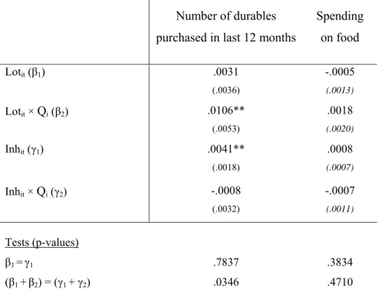
goods. Our falsification test compares the income response of spending on divisible nondurable consumption (food at home and in restaurants) to lottery wins and inheritances. If we see a difference in income effects between credit-constrained lottery winners and credit-constrained inheritors, but only for the indivisible goods in our data and not for indivisible goods, it will provide further support for the convexification hypothesis.

To implement our first, difference-in-difference test, we estimate an empirical model along the following lines:

(

1 2

)

(

1 2

)

'

it i it i it it it

d = β β+ Q Lot + γ γ+ Q Inh +α X +u (12)

Where dit is measure of durable purchases by agent household i at time t; Qi = 1 if

the agent is credit constrained, and equals 0 otherwise; Lotit and Inhit are financial

windfalls from lottery wins and inheritances, respectively; X_itis a vector of other

variables that might affect purchase of durables, including age, composition of household (couple, number of kids), home-ownership status, permanent income (proxied by

spending on food), employment status, financial expectations, year dummies, and u_it is a

random error term.

Previous empirical literature has shown that durables respond to unexpected windfalls (see Keeler, James and Abdel-Ghany, 1985), so we would expect that

0

1 1 =γ ≥

β . The theoretical considerations developed in the previous section suggest

that, among credit constrained households, selection into playing the lottery will lead to differential responses to a lottery win compared to other windfalls, in other words that

(

β1+β2

) (

≠ γ1+γ2

)

.

Our falsification test estimates a parallel model, with measures of nondurable (divisible) spending as the dependent variable.

To estimate our second, “small winnings” test, we estimate the following empirical model:

(

1 2

)

(

1 2

)

(

1 2

)

'

it i it i it i it it it it

d = β β+ Q Lot + γ γ+ Q Inh + δ δ+ Q SmLot ×Inh +α X +u

where SmLotit = 1 if someone receives a lottery win of less than £100, and equals 0

otherwise. Our hypothesis is that, among credit constrained households, those who

receive a medium-sized inheritance and also a small lottery win will not behave like

those who only received a medium-sized inheritance, ie.

(

δ δ1+ 2

)

≠0, but rather will

have the larger income responses of those who receive a medium-sized lottery win, i.e.

(

β β1+ 2

) (

=

(

γ γ1+ 2

) (

+δ δ1+ 2

)

)

.

4.2 Data

Our main analysis uses data taken from the British Household Panel Survey (BHPS) from 1997 – 2006 since this contains information on both durable purchases and financial windfalls. Beginning in 1991, this survey has annually interviewed members of a representative sample of around 5,500 households. On-going representativeness of the non-immigrant population is maintained by using a “following rule” – i.e. by following original sample members (adult and children members of households interviewed in the

first wave) if they move out of the household or if their original household breaks up.7

We select single and two-adult households where the head is aged 20 – 70. Our analysis sample contains information on 6,148 households (29,886 observations).

4.3 Descriptive Statistics

Consumer Durables

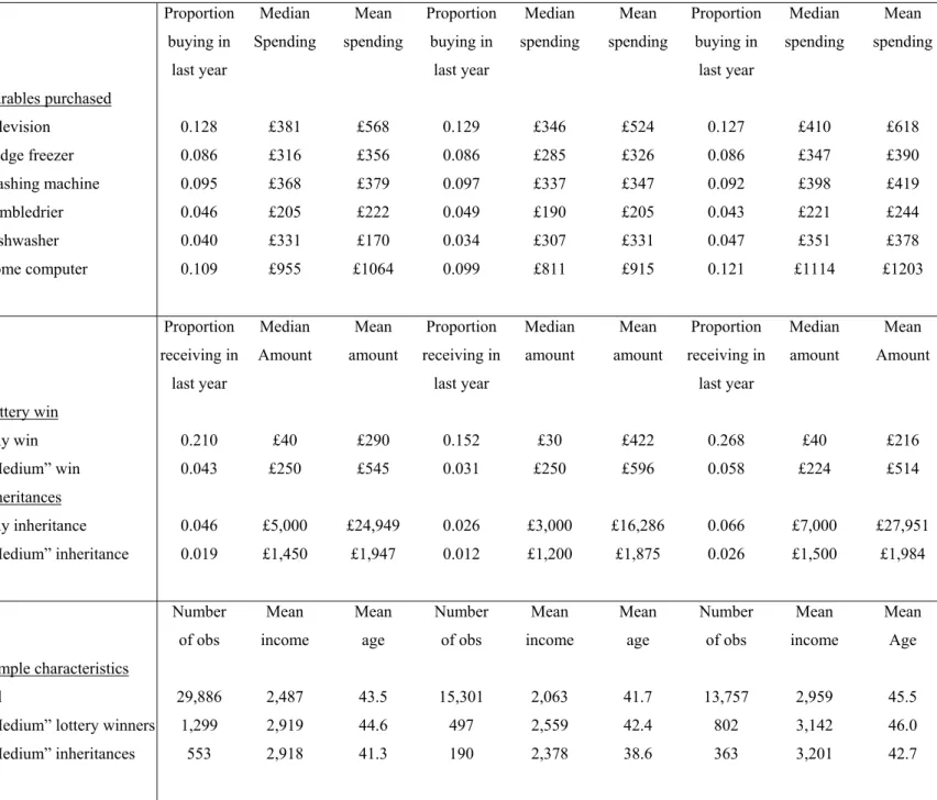
Information on purchases of consumer durables from the BHPS is given in Table 2. These are selected from a wider set of durables that households are asked about on the grounds that they are largely unchanged over the period and that they are genuinely “lumpy” to purchase new. This means we exclude, for example, VCRs which were becoming increasingly obsolete towards the end of the period and microwaves and CD players where the typical expenditure is fairly low. On average, 36% households had purchased at least one of the six durables over the previous year; 12% purchased two or more. In the case of most of the durables (except for dishwashers and home computers), they are bought by similar proportions of credit constrained and unconstrained

7 _{The survey incorporated booster samples from Scotland and Wales in 1999 and Northern Ireland in 2001,} but we restrict our sample to original sample members.

households. This is a set of basic durables that most households seek to replace on a regular basis, although credit constrained households typically spend less.

In principle, households could potentially smooth their spending on new durables. One possibility is renting, although this may be easier for some durables (televisions, for example) than for others (fridge-freezers). Also, most rental companies have a minimum rental period of 12 or 18 months and require a credit check, so the option of renting may not be open to everyone. Similarly, hire purchase companies also require a credit check and may charge high interest rates if the repayments are made over a long period.

Compared to these alternatives, buying a lottery ticket may not be an unattractive option.8

Credit Constraints

We define credit constrained households as those with no (income from) savings or investments. This is a broad definition by which around half of all households are constrained and will include some households who are not credit constrained in that they

can borrow, even if they have no savings.9 The benefit of our approach is that it yields

reasonable sample sizes in each of group. In sensitivity analysis, we have used narrower definitions that exclude anyone who owns their home and anyone with household income in the top two-third of the distribution and found similar results.

Lottery wins and inheritances

Since 1997, the BHPS has asked individuals whether they have received any of the following financial windfalls in the previous 12 months: a gambling win, an inheritance, a life insurance payment, a pension lump sum, a personal accident claim or a redundancy payment. Our comparison focuses on gambling wins (referred to here as

8 _{There are rental outlets that specifically target those with poor credit histories which do not require a} formal credit check, only five references. The advertised APR is 30%, but additional insurance which consumers are “strongly advised” to take out typically increases the effective rate of interest to more than 100% (Collard and Kempson, 2005).

9 _{Young and Waldron (2008) show that 16% of the UK population is credit constrained, according to} self-reported constraints in the amount that they could borrow, including both perceived constraints that

discouraged them from applying for credit, and actual constraints where the household was prevented from

borrowing either by the unavailability of credit or its high price. This is similar to Jappelli (1990) for the US who found that c. 20% of US households are credit constrained based on survey evidence that they have been refused credit, or put off applying for fear of refusal. In a different line of evidence, Alan and Loranth (2010) show that subprime borrowers – about 10% of the UK population – are insensitive to interest rate changes and hence likely credit constrained.

lottery wins since this is likely to be the case for most) and inheritances since the other windfalls may largely be anticipated (such as pension lump-sums), as we show below, and/or may be associated with events that directly affect the purchase of durables (such as

redundancy payments).10

Table 2 shows that the typical amounts received are fairly low for lottery wins and are much smaller than for inheritances. This is not surprising given the structure of

National Lottery payouts.11 However, this raises issues for our analysis; in particular, how

to ensure that we pick up the response to a lottery win compared to inheritance and not responses to different sized windfalls. Landsberger (1966) and Keeler, James and Abdel-Ghany (1985), for example, show that the size of the windfall affects what people do with it, with smaller windfalls being more likely to be spent.

Our approach is to focus on “medium-sized” windfalls of between £100 and £5,000. Anyone who receives a windfall of more than £5,000 in any wave is dropped from the analysis and in our initial analysis we ignore small (< £100) lottery wins and inheritances. Focusing on medium wins seems appropriate given our interest in consumer durables: larger wins may be associated with more widespread lifestyle changes such as moving house, while smaller wins may not be enough to finance the purchase of the white goods we focus on. Furthermore, restricting windfalls to this narrower range makes the average lottery win more comparable in size to the average inheritance. Within the range £100 - £5,000, lottery wins are still smaller on average than inheritances, as shown in Table 2, but the difference is much smaller. In sensitivity analysis (details available on request), we found similar results with narrower ranges of £100 - £1000 and £1,001 - £5,000.

Table 2 summarises separately average windfall payments for those who are credit constrained and those who are not. Many of those who are not credit constrained receive windfalls from lottery wins, and indeed a higher proportion than among those who are credit constrained. This is not inconsistent with people gambling to convexify, but is a reminder that this is only one of several possible motives for gambling. The

10_{We exclude any inheritances that are linked to widow(er)hood, i.e. deaths within the household that may} have an immediate effect on durable purchase.

11 _{The odds of winning £10 are 1:57, compared with odds of 1:1,031 to win around £100, 1:55,490 to win} around £1,000, 1:2,330,636 to win around £100,000 and 1:13,983,817 to hit the jackpot.

BHPS does not contain information on who has gambled and lost. To provide direct evidence on who gambles and how gambling varies with total expenditure, we use data from the 2007 UK Expenditure and Food Survey. Figure 4 shows that budget shares on gambling decline markedly with total expenditure, consistent with the need to gamble to convexify being concentrated among low income groups. Figure 4 also shows that the fraction of households with positive gambling expenditure is around 40% across a wide range of incomes, again consistent with the idea of there being more than one motive for gambling. In fact, the existence of lottery winners who are not credit constrained is necessary for the difference-in-difference strategy described above.

[Figure 4, about here]

Returning to Table 2, within the range we focus on (£100 - £5,000) there is no statistically significant difference in average windfall size between those who are potentially credit constrained and those who are not. Also, there is no statistically significant difference in household income between those who receive a medium-sized lottery win and those who receive a medium-sized inheritance. This is reassuring for our difference-in-difference specification.

[Table 2, Descriptive Statistics, about here]

5. Empirical Results

5.1. Main Results

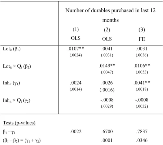
Our main results, addressing the question “Do durable purchases respond differently to lottery wins than to inheritances?”, are shown in Table 3. Column (1) presents the results of an OLS regression of durable purchases on lottery winnings, inheritances, and additional controls. We model the number of durables purchased during the previous twelve months as the dependent variable, but results are very similar using a binary indicator for whether or not the household purchased any durables. We include both lottery wins and inheritances as amount won (in £’000s) to deal with the fact that, even within our narrower range of “medium-sized” wins, the typical lottery win is quite a bit smaller than the typical inheritance.

The results indicate a significant response of durables purchases to a lottery win, but not to an inheritance. This is consistent with the convexification hypothesis, but, as described in the previous section this finding is also consistent with a number of alternative interpretations. In Column (2) we interact the windfall variables with a dummy variable indicating whether the agent is credit constrained. This corresponds to equation (12) above and implements our main “difference-in-different” test. The results show that the propensity to purchase durables out of (endogenously-selected) lottery wins is significantly greater than the propensity to purchase durables out of an (exogenously-determined) inheritance for households that are credit constrained. By contrast, there is no significant difference among unconstrained households. In Column (3) we show that these results are robust to the inclusion of individual fixed-effects.

[Table 3 about here]

The convexification hypothesis is a selection mechanism that operates on variables (the need for durables, cash on hand) that vary through time, and that operates only for the credit-constrained. The results in Column (3), which allow for fixed effects in estimating income effects, and which double-difference income effects (across the constrained and unconstrained, and across inheritors and lottery winners), rule out any alternative selection mechanism which operates on time invariant unobservables, and any selection mechanism which is not limited to the credit constrained.

5.2. Are Inheritances Anticipated?

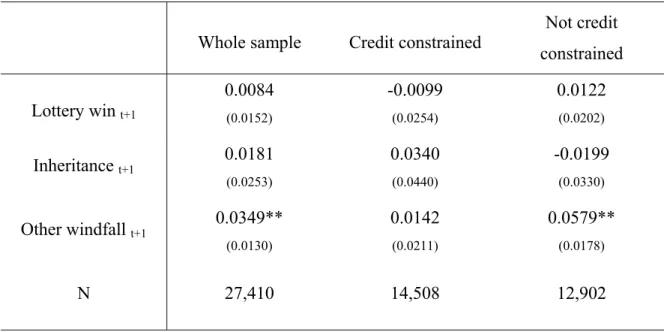
As noted in the previous section, one potential concern is that inheritances may differ from lottery wins in being reasonably well anticipated by the individual. However, there is no evidence of households adjusting either their financial expectations or their durable purchases ahead of receiving an inheritance. Table 4 reports the results of a fixed effects regression of a binary indicator for whether the (head of the) household expects their financial situation to improve over the next 12 months on a set of indicators for whether or not the household does in fact receive a lottery win, an inheritance or one of the other financial windfalls (life insurance payment, pension lump sum, personal

accident claim, redundancy payment) over the following 12 months, focusing on medium-sized windfalls (between £100 - £5,000). Only the coefficient on other windfalls is positive and significant; medium inheritances do not appear to be anticipated. Consistent with this, sensitivity analysis (details available on request) that included lead terms in the regression analysis to pick up the effect of any anticipated windfalls found no significant effects.

[Table 4 about here] 5.3. The Small Winnings Test

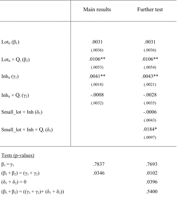
Section 4 proposed a second test of the convexification hypothesis based on the idea that individuals who receive an inheritance but whom we know to have been gambling (because they report very small winnings) should behave like lottery winners (rather than like inheritors). The results in Table 5 show that this is exactly what we find in our data. Column (1) reproduces (from Column (3) of Table 3) our main difference-in-difference with individual fixed effects results, corresponding to equation (12). In Column (2) we report estimates of equation (13) in which we interact the inheritances variables with a dummy indicating whether the agent reported a small lottery win. We find that credit-constrained inheritors that we know to have been gambling exhibit much larger income effects than other inheritors. In fact, their responses are not statistically different from the lottery winners. This test provides further confirmation that our findings in the previous section were not driven by differences in the way individuals respond to lottery winnings compared to inheritances. Instead, it is the characteristics and situation of the person who receives the money that matters. Credit-constrained gamblers have larger responses and this is consistent with the idea that they are a selected group: close to a purchase margin.

[Table 5 about here] 5.4. Falsification Test

Finally, in Table 6 we provide a falsification test based on the fact that the convexification hypothesis should generate differences in income effects only for indivisible goods. We therefore run the same regression but include weekly household

spending on food on the left-hand side.12 Consistent with the convexification hypothesis and with the predictions of a standard life-cycle model, we find zero income effects for both lottery wins and inheritance receipts when we examine food spending.

[Table 6 about here]

Overall, our empirical results are fully consistent with the theory presented in Section 2 and lend strong support to the idea that consumers gamble to convexify.

6. Conclusion

This paper sheds light on why risk averse individuals gamble. We find that purchases of durables are more responsive to lottery winnings than to inheritances and argue that this difference in durable purchase is consistent with individuals gambling to convexify. We find this difference while controlling for individual fixed effects; we find it only for households who are credit-constrained who might have an incentive to gamble; and we find it only in expenditures on indivisible goods. Moreover, we find that an inheritance has a larger effect when received by individuals who were playing the lottery: it is who receives the money, rather than the source of the money, that matters. These multiple lines of evidence are all consistent with gambling to convexify: the larger income effects associated with lottery winnings result from the fact that it is exactly those who are close to a purchase threshold who choose to gamble. It is hard to think of another plausible explanation that is consistent with all these multiple lines of evidence.

Our findings are important for a number of reasons. First, our finding highlights the difficulty of finding appropriate instruments – in this case for income. The random success of winning a lottery would seem to make it a natural instrument for unanticipated income changes that should allow for the identification of income effects, as in Imbens et al. (2001). In their conclusion, Imbens et al. (2001) note the caveat that they have “no direct evidence concerning the difference of responses to lottery income versus other sources of unearned income” (page 793). We provide both evidence of and economic motivation for such differences. The decision to play lotteries is itself an economic

decision that is not independent of the income effect on winning: those who choose to play lotteries will display larger income effects than the rest of the population, as our data confirm.

Second, and more fundamentally, our findings provide at least a part of the explanation for gambling among low-income households, and also the popularity of so-called prize-linked savings products amongst these households. Of course, there are other reasons for people to gamble besides convexification. Recently, it has been suggested that prize-linked savings products could be used to promote saving through the “excitement factor” and this may be an important factor for many. However, our research points to another potential reason why such products might appeal to low-income households; they may allow consumers to overcome indivisibilities potentially more quickly than conventional savings products. On the other hand, given the poor return to playing lotteries, our evidence that individuals are gambling to finance indivisible purchases highlights the lack of financing options available to poor households, and the severity of the credit constraints they face.

Finally, our evidence on how individuals deal with non-convexities provides guidance on how we should model the behaviour of those individuals in structural models. In particular, the appropriate way to model optimisation by individuals in the presence of non-convexities is to allow those individuals to play lotteries.

REFERENCES

Alan, S. and G. Loranth, (2010). “An Empirical Analysis of Subprime Consumer Credit Demand.”

Appelbaum, E. and E. Katz, (1981), “Market Constraints as a Rationale for the

Friedman-Savage Utility Function.” The Journal of Political Economy, Vol. 89, No. 4

(Aug., 1981), pp. 819-825.

Attanasio, O., Low, H. and V. Sanchez-Marcos, (2008) “Explaining changes in female

labour supply over the life-cycle” The American Economic Review, Vol

98(4):1517-1552

Bailey, Martin J., Mancur Olson, and Paul Wonnacott (1980). "The Marginal Utility of Income Does Not Increase: Borrowing, Lending, and Friedman-Savage

Gambles," The American Economic Review, vol. 70, no. 3, June 1980, pages

372-379.

Besley, Timothy, Stephen Coate, and Glenn Loury (1993). "The Economics of Rotating

Savings and Credit Associations," The American Economic Review, vol. 83, no. 4,

September 1993, pages 792-810.

Collard, Sharon and Kempson, Elaine (2005) Affordable Credit: The way forward, Bristol: Policy Press

Danforth, J., (1979) "On the role of consumption and decreasing absolute risk aversion in the theory of job search" In: Lippman, S. and McCall, J. (Eds.) Studies in the Economics of Search. North Holland, New York

Epley, N., & Gneezy, A. (2007). The framing of financial windfalls and implications for public policy. Journal of Socio-economics, 36, 36-47

Farrell, L., Hartley, R., Lanot, G. and Walker, I.. (2000) The Demand for Lotto: the Role

of Conscious Selection.” Journal of Business and Economic Statistics, vol. 18, pp.

228-241.

Flemming, J.S. (1969). "The Utility of Wealth and the Utility of Windfalls," The Review

Friedman, M. and L. J. Savage (1948) "The Utility Analysis of Choices Involving Risk"

Journal of Political Economy, 56(4): 279-304

Gardner and Oswald (2007) Money and Mental Wellbeing: A Longitudinal Study of

Medium-Sized Lottery Wins, Journal of Health Economics, vol. 26(1), pages

49-60

Gomes, Joao, Jeremy Greenwood, and Sergio Rebelo (2001), "Equilibrium

Unemployment," Journal of Monetary Economics, Vol. 48, pp. 109--152.

Handa, S. and Kirton, C., (1999), “The economics of rotating savings and credit

associations: Evidence from the Jamaican ‘Partner’” Journal of development

Economics, 60:173–194.

Hansen, G. (1985) "Indivisible labor and the business cycle" Journal of Monetary

Economics 16: pp. 309—328

Hartley, R. and Farrell, L. (2002) Can Expected Utility Theory Explain Gambling?

American Economic Review, vol 92(3) pp. 613-624.

Holtz-Eakin, Douglas, David Joulfaian; Harvey S. Rosen The Carnegie Conjecture:

Some Empirical Evidence The Quarterly Journal of Economics, Vol. 108, No. 2.

(May, 1993), pp. 413-435.

Heckman, J.J. and J.A. Smith, (1995), “Assessing the Case for Social

Experiements.”Journal of Economic Perspectives, 9(2):85-110

Hurst, E. and Lusardi, A. (2004) “Liquidity constaints, household wealth and entrepreneurship”, Journal of Political Economy, vol 112, pp. 318-47

Imbens, G., D.B. Rubin and B.I. Sacedote, (2001), “Estimating the Effect of Unearned

Income on Labor Earnings, Savings, and Consumption: Evidence from a Survey of Lottery Players.” The American Economic Review, 91(4):778-794

Jappelli, T. (1990). ‘Who is Credit Constrained in the U.S Economy’, Quarterly Journal

of Economics, Vol. 105(1), pp. 219-262.

Joulfaian, David, and Mark O. Wilhelm. 1994. "Inheritance and Labor Supply." Journal

Keeler, James and Abdel-Ghany (1985) “The relative size of windfall income and the

permanent income hypothesis”, Journal of Business and Economic Statistics, vol

3, no. 3, pp. 209-215

Kearney, Peter Tufano, Guryan, and Erik Hurst (2010) “Making Savers Winners: An Overview of Prize-lined Savings Products.” NBER Working Paper 16433.

Kreinin (1961) “Windfall income and consumption – additional evidence” American

Economic Review, June 1961, pp.

Landsberger, M. (1966), "Windfall Income and Consumption: Comment," The American

EconomicReview, 56: 534-40

Levav and McGraw (2006) “Emotional Accounting: Feelings About Money and Consumer Choice.” Columbia Business School Working Paper, 2006.

Lentz, R. and T. Tranaes (2005), "Job Search and Savings: Wealth Effects and Duration

Dependence", Journal of Labor Economics, 23(3), 467-490.

Milkman, Katherine L., John Beshears, Todd Rogers, and Max H. Bazerman (2007) “Mental Accounting and Small Windfalls: Evidence from an Online Grocer”. Harvard business School Working Paper

Ng, Yew-Kwang (1965). "Why Do People Buy Lottery Tickets? Choices Involving Risk

and the Indivisibility of Expenditure," The Journal of Political Economy, vol. 73,

no. 5, October 1965, pages 530-535.

Parker, J. (1999) The Reaction of Household Consumption to Predictable Changes in

Social Security Taxes American Economic Review, September 1999, pp. 959-973

Prescott, E. C. and R. M. Townsend (1984) General competitive analysis in an economy

with private information, International Economic. Review. 25: 1—20

Prescott, E. C. and R. M. Townsend (1984) Pareto optima and competitive equilibria with

adverse selection and moral hazard, Econometrica 52: 21--45.

Rogerson, Richard (1988) "Indivisible labor, lotteries and equilibrium" Journal of

Souleles, N. (1999) The Response of Household Consumption to Income Tax Refunds

American Economic Review, September 1999, pp. 947-958

Taylor, Mark (2001), 'Self-employment and windfall gains in Britain; evidence from

panel data', Economica, 68, #272, November, pp. 539-565.

Townsend, Robert M. & Kenichi Ueda (2006) "Financial Deepening, Inequality, and

Growth: A Model-Based Quantitative Evaluation," Review of Economic Studies,

vol. 73(1), pages 251-293.

Tufano, Peter (2008). ‘Savings Whilst Gambling: An Empirical Analysis of U.K.

Premium Bonds.’ American Economic Economic Review Papers and

Proceedings, 98(2): 321-26.

Young, Garry and Waldron (2006) The state of British household finances: results from the 2006 NMG Research Survey, bank of England Quarterly Bulletin, Q4 pp. 397-403

Appendix: Proofs of Results 2 and 3 Proof of Result 2

Result 2: Lottery tickets are not purchased outside the interval x₁ x*₂ 1 q,x*₂ 1 q

⎡ − ⎤

∈_⎢ − + _⎥

⎣ ⎦.

Proof:

The value functions for not buying a lottery ticket is given by:

( )

* 0 1 1 2 1 * 1 1 2 if ( ) if l u x x x V u x p η x x = _{= ⎨}⎧ < − + ≥ ⎩

The expected value function for buying a ticket is given by:

(

)

* 1 1 2 * 1 1 1 2 1 * 1 1 2 * 1 1 2 1 1 if 1 if 1 (1 ) ( 1 ) ln if 1 1 1 ( ) if l q q u x x x u x x x q q E V q q u x p x x q q u x p x x q q η η = ⎧ ⎛ ₊ − ⎞ _{< −} − ⎫ ⎪ ⎜ ⎟ ⎪ _{⎧ − < + ⎫} ⎪ ⎝ ⎠ ⎪ ⎡ ⎤ = _{⎨ ⎬}+ − _{⎨ ⎬} ⎣ ⎦ _{− − − − + ≥ +} ⎩ ⎭ ⎪ _{+ − + ≥ −} ⎪ ⎪ ⎪ ⎩ ⎭

Now consider separately the incentive to buy a lottery ticket when cash-on-hand is below the interval and above the interval.

1) When

(

)

*

1` 2 1 ,

x <x − −q q

cash-on-hand in period 2 will be sufficiently low that even if the lottery is won, *

2 2

x <x ,

and so the household does not buy the indivisible good, regardless of the lottery outcome. Thus, the expected value of buying a lottery ticket becomes:

(

)

1 1 1 1 1 (1 ) 1 l q E V qu x q u x q = ⎛ − ⎞ ⎡ ⎤ = _⎜ + _⎟ + − − ⎣ ⎦ _{⎝ ⎠}

The value of not buying becomes: 0

( )

1 1

l

V = =u x . Since the gamble is actuarially fair and

utility, u, is concave, the value of not buying a lottery ticket is always greater than the expected value of buying the lottery ticket:

( )

(

)

0 1 1 1 1 1 1 1 (1 ) 1 . l l V u x q qu x q u x E V q = = = ⎛ − ⎞ _{⎡ ⎤} ≥ _⎜ + _⎟ + − − = _{⎣ ⎦} ⎝ ⎠ 2) ) When * 1` 2 1, x >x +

cash-on-hand in period 2 will be sufficiently high that even if the lottery is lost, *

2 2

x >x ,

and so the household buys the indivisible good regardless of the lottery outcome. Thus, the expected value of buying a lottery ticket becomes:

(

)

1 1 1 1 1 (1 ) 1 l q E V qu x p q u x p q η = ⎛ − ⎞ ⎡ ⎤ = _⎜ + − _⎟ + − − − + ⎣ ⎦ _{⎝ ⎠}

And the value of not buying becomes:

(

)

0

1 1

l

V = =u x −p +η

Since the gamble is actuarially fair and utility, u, is concave, the value of not buying the lottery tickey is always greater than the value of buying the ticket.

(

)

(

)

0 1 1 1 1 1 1 1 (1 ) 1 , l l V u x p q qu x p q u x p E V q η η = = = − + ⎛ − ⎞ _{⎡ ⎤} ≥ _⎜ − + _⎟ + − − − + = _{⎣ ⎦} ⎝ ⎠ Proof of Result 3

Result 3: There exists a region, x1∈ ⎣⎡x x1, 1⎤⎦, which contains * 2

x

(

x1<x2*<x1

)

, in which

the agent will purchase a lottery ticket.

Proof:

We consider the incentive to buy a lottery ticket in the region of *

2

x . Define the