Machine Learning vs Conventional Analysis Techniques for the Earth’s Magnetic Field Study

(1)

Machine Learning vs Conventional Analysis

Techniques for the Earth’s Magnetic Field Study

Sheri Loftin

Southern Methodist University, [email protected]

Sarah J. Fite

Laura V. Bishop

Stavros Kotsiaros

University of Maryland, [email protected]

Follow this and additional works at:

https://scholar.smu.edu/datasciencereview

Part of the

Categorical Data Analysis Commons

, and the

Other Earth Sciences Commons

Recommended Citation

Loftin, Sheri; Fite, Sarah J.; Bishop, Laura V.; and Kotsiaros, Stavros (2019) "Machine Learning vs Conventional Analysis Techniques for the Earth’s Magnetic Field Study,"SMU Data Science Review: Vol. 2 : No. 1 , Article 7.

(2)

Machine Learning vs Conventional Analysis Techniques

for the Earth’s Magnetic Field Study

Sheri Loftin

1

, Sarah Fite

2

, Laura Bishop

3

, Stavros Kotsiaros

4 1_{Master of Science in Data Science, Southern Methodist University,}

Dallas, TX 75275 USA

2_{National Aeronautics and Space Administration, Goddard Space Flight Center,}

8800 Greenbelt Drive, Greenbelt, MD 20771 USA {sloftin, fites, lvbishop}@smu.edu

[email protected]

Abstract. Current techniques for calculating and generating models used for

analyzing the Earth’s magnetic field are laborious and time-consuming. We assert that machine learning can have a significant impact on building magnetic field models more quickly and on various levels of complexity, specifically as it pertains to data cleansing and sorting. Our approach to this problem uses a reverse iterative multi-phase process for data cleansing, in which, initially, the CHAOS-6 model data is examined to determine if machine learning can be used to differentiate between useful data components for spherical harmonics, versus data noise. During this phase, six different machine learning techniques are used and compared: two classification techniques (Convolutional Neural Network (CNN) and Support Vector Classification (SVC)) and four regression techniques (Random Forest Regression (RFR), Support Vector Regression (SVR), Logistic Regression, and Linear Regression). During this initial phase, the focus is on understanding the accuracy of machine learning for model selection and uses relatively clean data. Future phases should include machine learning relevance as it pertains to the massive volume of data received from satellites. Exploring the machine learning capabilities for magnetic field datasets accomplishes 1) faster and more efficient computation when there are millions of rows of data in any given 30-day period, and 2) lowers the propagation of errors that cause some data to be useless in the spherical harmonics computations used in the model generation.

1_{Sheri Loftin is completing her MS in Data Science at SMU. She is the Planetary Data}

Systems Database Training and Communications Coordinator at Goddard Space Flight Center, contracted through Adnet Systems.

2_{Sarah Fite is completing her MS in Data Science at SMU. She is a Business Analyst at}

iHeartMedia, Inc.

3_{Laura Bishop is completing her MS in Data Science at SMU. She is a Technical Sales}

Manager in Cybersecurity at IBM.

4_{Dr. Stavros Kotsiaros is the advisor for this project. He is a research scientist at the}

(3)

1 Introduction

The European Space Agency’s (ESA) Living Planet Programme launched a trio of satellites on 22 November 2013 called Swarm, which is the fourth Earth Explorer mission [5].

Two years of magnetic data from the Swarm mission and monthly means from 160 ground observatories were used in the paper by Finlay et al., Recent geomagnetic secular variation from Swarm and ground observatories as estimated in the CHAOS-6 geomagnetic field model, (2016) [19].

The Earth’s magnetic field is effectively a‘super shield’ that protects the planet from cosmic radiation and charged particles in the solar wind [6]. Earth’s magnetic field is created by sources both internal and external to our planet. The largest field is created by electric currents flowing in the Earth’s liquid outer core which is known as the “core field”. The core field together with a small contribution from the magnetized rocks in the Earth’s lithosphere producing what is known as the lithospheric or crustal field, encompass the so-called internal magnetic field. The external field is produced by electric currents flowing in the Earth’s ionosphere and magnetosphere.

Low Earth Orbiting (LEO) satellites measure the Earth's large scale lithospheric magnetic field. LEO satellites provide a statistical homogeneity of measurement on a world-wide scale. In reality, the lithospheric magnetic signal is masked by the dominant core field signal as well as by the “time-varying external fields” that contaminate the lithospheric signal along the satellite’s orbit [5]. There are ways to minimize the contamination by suppressing the undesired signals with ‘ along-satellite-track’ analysis [7][8] or using magnetic field gradients [29]. Specifically, the configuration of the Swarm trio can be used to estimate the East-West (EW) magnetic field gradient from differences between measurements of the two lower satellites, and the North-South gradient from differences between successive vector measurements along the satellite tracks [5]. A major statistical and data challenge is extracting weak lithospheric signals from the total magnetic field observations [5]. Modeling the magnetic field due to both the internal and external sources is essential for a more complete and more accurate estimation of the Earth’s total magnetic field. The CHAOS-6 [19] model incorporates lithospheric, core and external field sources. Even with the most accurate satellite measurements, developing a precise model for the Earth’s magnetic field is difficult from a few perspectives: field of study, statistical, and data. It requires expertise in a number of different scientific disciplines, including magnetometry, spacecraft measurements, planetary physics, geology, etc. As in many complex scientific fields of study, the more professional experience gained, the better the results. A benefit of studying the Earth's magnetic field is the plethora of data collected. For example, in this study, 31 days of satellite data generated over 2.6 million rows of cleaned collection data representing 2.6 million data points of magnetic field readings. Current methods struggle to handle the amount of data produced. Another limitation of the current methods lies in a shortcoming within spherical harmonic computations. "Dirty data" entered into the spherical harmonic computation creates errors that do not only affect the region of the Earth where the

(4)

contamination originated but globally. Therefore, the errors propagate throughout the model and may affect the usefulness of the model in specific regions of interest. With spherical harmonics, the errors cannot be all filtered out, and some of the data rendered useless as the propagation of such errors may become significant and affect the weaker signals to be modelled. With more modern machine learning techniques, these errors can be detected and filtered out earlier, thereby allowing more of the data to be used and lowering the overall error leakage in the model. These techniques are how tools, technology, and processing of Data Science and Machine Learning can improve the generation of geomagnetic field models better for all scientists.

2 Background

The goal for studying the Earth’s magnetic field is two-fold: 1) to better understand the magnetic shield and 2) to study the interior of our planet. Pragmatic applications for this research include understanding of tectonic dynamics, drilling for natural resources, planetary science, and better navigation systems. While the theoretical perspective paints a dire picture of a weakening magnetic shield, the more that is known and understood, the better our advances to understand the implications of such change. The objective for applying Data Science approaches and Machine Learning techniques to creating geomagnetic models is to reduce the complexity of generating hi-resolution models to be used in the study of the Earth’s magnetic field and to utilize the enormous amount of collected data, thereby allowing for a more accurate view of the geomagnetic field. Today, hi-resolution models require extensive computations with several iterations making the model generation an expensive process.

The design of this project is to improve the management of the data volume by reducing the compilation time by at least 30%. Additionally, we aim to improve the error propagation and leakage in the analysis and estimation due to the entanglement of the various magnetic field sources. Finally, another goal is to use more of the data collected to provide a more thorough model.

2.1 Definition of Terms

The Swarm satellite configuration consists of two satellites which orbit 450-Kilometers above the Earth and a third satellite which orbits at 530-Kilometers above the Earth. At the core of each Swarm satellite is an instrument, the Vector Field Magnetometer (VFM), which is pertinent to this study:

Vector Field Magnetometer (VFM) – Located at the tip of the optical bench on the boom, the VFM measures magnetic field vector. The VFM contains a 3-axis Compact Spherical Coil (CSC) sensor with a 3-axis Compact Detector Coil (CDC) sensor inside that acts as a closed loop system. It achieves a null field at the detector coils in the sphere by adjusting the compensating CSC currents. The raw data is the current level in the CSC coils.

The geomagnetic field is modelled in terms of Spherical Harmonics. A model of the Earth’s magnetic field is therefore a set of spherical harmonic coefficients which aim to represent as accurate a picture as possible of the current state of the geomagnetic field of Earth.

(5)

3 Dataset and Data Exploration

The data we are using consists of 2,678,400 rows of cleaned, magnetic data produced by the CHAOS-6 model. This “dummy” data will allow the model to be trained for “best fit” in the Crustal data model.

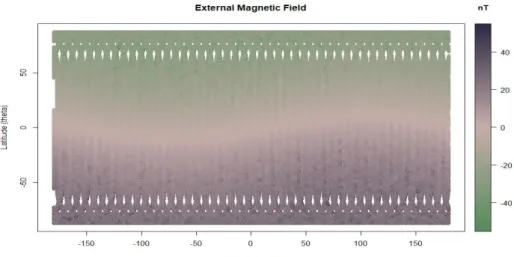
There are 19 variables collected as shown in Table 1.

Table 1 CHAOS-6 Model Data used for comparison

Variable Name Meaning Minimum Maximum

T [md2000] Time in units of decimal

DAYS from 1/1/2000 midnight.

5844 5875

r [km] Coordinate distance from the

center of Earth measurements

– radius in kilometers (km)

6814 6835

theta [degrees] Position coordinate angle from x-axis – in

degrees(Longitude)

2.648 177.352

phi [degrees] Position coordinate angle from z- axis – in degrees(Latitude)

-180.0000 179.9995

B_r1 [nano Tesla] Radial Internal Field (I) -48793 52931

B_theta1 [nanoTesla] Co-latitudinal Internal Field (I)

-32958 11531

B_phi1 [nanoTesla] Azimuthal Internal Field (I) -12785.80 12282.23

B_r2 [nano Tesla] Radial core Field (C) -48792 52934

B_theta2 [nanoTesla] Co-latitudinal core Field (C) -32957 11528

B_phi2 [nano Tesla] Azimuthal core Field (C) -12786.330 12281.600

B_r3 [nano Tesla] Radial crustal Field (L) -15.34000 12.67000

B_theta3 [nano Tesla] Co-latitudinal crustal Field

(L) -7.73000 11.38000

B_phi3 [nano Tesla] Azimuthal crustal Field (L) -10.62000 7.83000

B_r4 [nano Tesla] Radial external Field (E) -55.1600 54.960

B_theta4 [nano Tesla] Co-latitudinal external Field (E)

-12.39 114.08

B_phi4 [nano Tesla] Azimuthal external Field (E) -27.0000 24.6300

B_r5 [nano Tesla] Radial total Field (T) -48824.1 52963.3

B_theta5 [nano Tesla] Co-latitudinal total Field (T) -32952 11540

(6)

Formula background- Magnitude of the magnetic field is computing using a 3D variation of the Pythagorean Theorem:

𝐵 = √𝑥 ∗ 𝑥 + 𝑦 ∗ 𝑦 + 𝑧 ∗ 𝑧

𝐼𝑛𝑡𝑒𝑟𝑛𝑎𝑙 𝐹𝑖𝑒𝑙𝑑 = 𝐶𝑜𝑟𝑒 𝐹𝑖𝑒𝑙𝑑 + 𝐶𝑟𝑢𝑠𝑡𝑎𝑙 𝐹𝑖𝑒𝑙𝑑

𝐼𝑛𝑡𝑒𝑟𝑛𝑎𝑙 𝐹𝑖𝑒𝑙𝑑 = [𝐵_𝑟2, 𝐵_𝑡ℎ𝑒𝑡𝑎2, 𝐵_𝑝ℎ𝑖2] + [𝐵_𝑟3, 𝐵_𝑡ℎ𝑒𝑡𝑎3, 𝐵_𝑝ℎ𝑖3]

𝑇𝑜𝑡𝑎𝑙 𝐹𝑖𝑒𝑙𝑑 = 𝐼𝑛𝑡𝑒𝑟𝑛𝑎𝑙 𝐹𝑖𝑒𝑙𝑑 + 𝐸𝑥𝑡𝑒𝑟𝑛𝑎𝑙 𝐹𝑖𝑒𝑙𝑑 𝑇𝑜𝑡𝑎𝑙 𝐹𝑖𝑒𝑙𝑑 = 𝐼𝑛𝑡𝑒𝑟𝑛𝑎𝑙 𝐹𝑖𝑒𝑙𝑑 + [𝐵_𝑟4, 𝐵_𝑡ℎ𝑒𝑡𝑎4, 𝐵_𝑝ℎ𝑖4]

The design is based on using the crustal field variables, 𝑟 𝑡ℎ𝑒𝑡𝑎 𝑝ℎ𝑖, to represent the position of the measurement and the strength of the magnetic field at that position. A machine learning model is created to yield the same or statistically similar enough results for the crustal field variables in data columns 11-14.

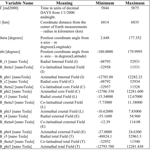
As shown in figures 1 and 2 (below), each magnetic field source has its own "signature" and varies significantly in strength, as compared to the other. In each figure the x-axis represents longitude, and the y-axis represents latitude, while the color bar represents the strength of the magnetic field at each location. The unit for the color bar is nanoTesla. Also, in each figure, North is 0 on the y-axis and South is 180; thus the Earth appears upside down.

The total magnetic field has definite features, especially around the polar regions of the Earth. This is dominated by the most robust magnetic field source of the Earth and is created by the dynamo action of our solid core rotating at a slightly different speed than the surrounding liquid mantle.

Fig. 1. 2D rendering of the core magnetic field with the ‘x' axis for longitude and ‘y' axis for

(7)

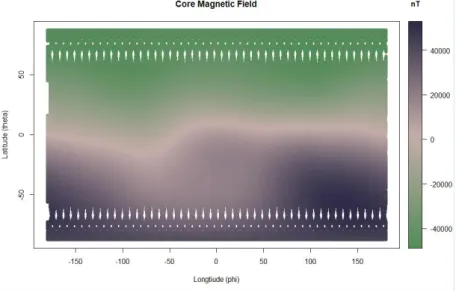
Within the data of the crustal field, the continental outlines are subtle but present. The strength of the magnetic field at each point is significantly lower than the strength of the core field. Because of this vast difference, the signal of the crustal field can easily get lost within the data of the total magnetic field, which includes the core field, the crustal field, and the external field.

Fig. 2. 2D rendering of the crustal magnetic field with the ‘x' axis for longitude and ‘y' axis for

latitude.

Since the core field is so much stronger than the crustal field (the signature we are looking to model with this project), we have chosen to use the combination of the external field and the crustal field as our dataset. The goal is to be able to search through this dataset and have the machine learning tool find the signature of the crustal magnetic field.

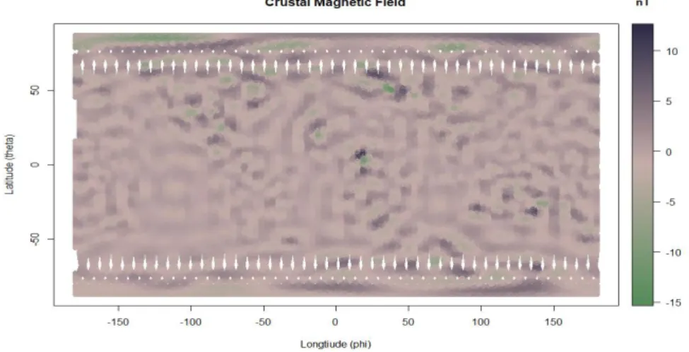
The external field is produced in the ionosphere and the magnetosphere of the Earth and is only one factor stronger than the crustal field. On the contrary, in comparison, the core field is three factors stronger. The external field also lacks the variety of anomalies that exist within the crustal field.

(8)

Fig. 3. 2D rendering of the external magnetic field data with the ‘x' axis for longitude and ‘y' axis

for latitude.

4 Methodology

4.1 Model Comparison

Initially, the model is trained using the variables related to time, position and the positional components of the total magnetic field. These variables correspond to columns 1-4 and 17-19 and are labeled t, r, theta, phi, and B_r5, B_theta5, and B_phi5. Columns 1-4 feeds the algorithm and resulting in Columns 17-19. This is the proof of concept to justify using Swarm mission data to test the applicability of a machine learning dataset for magnetic field modeling.

4.2 CHAOS-6 Analysis Techniques

The CHAOS-6 model uses a method called spherical harmonics. The model itself is a series of coefficients that when entered into the spherical harmonic formula produce a description of the magnetic field of the Earth.5

The crustal field is represented by the coefficients corresponding to 21 – 110 degrees. There are 11,880 coefficients in the CHAOS-6 model. Given the complexity of the process and the vast number of coefficients, it becomes easy to see why this process would take so long to compute values.

5_{An introduction to spherical harmonics by Wojciech Jarosz, Assistant Professor at Dartmouth}

University is found at

(9)

4.3 Machine Learning Methods

As previously mentioned, this paper examines six (6) machine learning approaches to determine which method best predicts the data most useful for the crustal data model. The approach taken is an inverse data analysis. That is, instead of starting the process with the dirtiest data imported directly from the source (satellite data), then struggling with cleansing and clustering that data, then spending a great deal of time determining if errors and challenges encountered during that process are the result of the premise or a challenge in the data, we chose to start with a clean, known dataset (crustal model). This dataset is then mixed with the external model data to create our initial phase of 'dirty data.' Our premise is that if the crustal model data is successfully predicted amongst the “dirty data” of the external model data, success is achieved at this initial phase (Phase 1). Following this, the next step is to use the dataset in a dirtier, earlier revision from the satellite. The number of backward iterations of the data from clean to dirtier is not known at this time but is estimated to be at least four (4) to confidently know this approach is statistically successful and useable by NASA Goddard.

We review both classification and regression methods. Phase 1 is looking at predicting ‘in or out' of the crustal dataset, which is standard classification. Due to the highly linear nature of the data, and unknown characteristics of the data in following Phases (closer to the raw data from the satellite), the requirement exists to have a strong machine learning foundation by which to evaluate the best method.

Classification Approaches. Classification approaches are essential in systematically structuring the data.

Convolutional Neural Networks. Research into previous machine learning techniques used to improve upon spherical harmonics shows that Convolutional Neural Networks (CNN) have potential. While no previous research has been discovered discussing this from a planetary magnetic field perspective, there have been attempts to replace spherical harmonics in other realms. Two papers listed below have used CNN to replace spherical harmonics in the realms of particle physics [21] and heart MRIs [22]. By design, the CNN technique is the starting point because of its ability to handle image data, before any data analysis had been conducted. SVC, RFR, SVR, Logistic Regression, and Linear Regression act as comparison techniques to determine which method yields the best statistical result of accuracy.

(10)

Fig 4: Outline of continents overlaid on the crustal field model data. Courtesy of Stavros Kotsiaros.

CNN's primary use is image analysis. In this case, CNN treats the magnetic field of the Earth as an image with certain distinctive features. As seen in Figure 4 above, the outlines of the continents are somewhat visible to a trained eye. This feature could be used to distinguish the image of the crustal model from the image of the core or the external model. A CNN should be able to separate this signature feature.

Support Vector Classification. Given the linear nature of the data, SVC is as a secondary approach for comparison of CNN.

Regression Approaches. For each regression approach, the measure of a proper machine learning technique is its error rate. The top three (3) error techniques according to Botchkarev survey [27] are used in this paper to evaluate the distance between estimates and predictions during cross-validation:

1) Mean Absolute Error (MAE) – Average of absolute distance between data and prediction. The proportional weight of the error. Less sensitive to outliers. 2) Root Mean Square Error (RMSE) – Measures average magnitude of error. Gives

weight to larger errors and makes them more pronounced in the model; useful to compare to MAE to understand the distribution of the larger errors. When MAE = RMSE, the distribution of errors is consistent.

3) Mean Absolute Percentage Error (MAPE) – This measurement shows a small relative error and shows the precision of the models. This works best with medium and large datasets.

(11)

The model analysis Python code used was built by Dr. Jacob Drew of Southern Methodist University and his work for the State of North Carolina Education [23]. The model analysis code builds regression models that are evaluated using cross-validation and a random seed. This is accomplished using parameters of Python's sklearn.model_selection's cross-validate function, which performs the cross-validation for regression estimators. The random seed ensures that all regression estimators are tested on the same randomly selected data rows for each cross-validation fold. Dr. Drew created custom scorers for MAE, RMSE, and MAPE using the three chosen mean error scores. Thus, all three scores are calculated using a single call to cross-validate(). All of this functionality lies in a custom function 'EvaluateRegressionEstimator(),' which allows multiple regression models to be tested using the same test/train cv data and consistently produces the evaluation scores for each model.

The same regression model function was used to evaluate each approach outside of CNN and SVC. A five (5) fold cross validation is used, along with passing the three (3) mean error scores into the cross-validation in one (1) call.

GridSearchCV "exhaustively" searches for the best parameters used in the regression methods for the four (4) non-CNN regression approaches. GridSearchCV is passed as a regression algorithm (one of the 4), a parameter grid based on the regression, and a number of cross-validation folds. Using GridSearchCV improves the accuracy of nested cross-validation, thereby improving the accuracy of the model prediction. Linear Regression models the behavior between dependent response (label of 'in crustal model' - 1 or not - 0) and explanatory variables of 'theta', 'phi' and 'mag' (magnitude).

For these approaches, a sample size from the 2.6 million Swarm satellite model data was used totaling 26,784 rows and five (5) folds. The training set is 21,427 rows, and the test set is 5,357 rows. This smaller dataset was chosen to allow for decent processing time on a 2016 MacBook Pro running macOS Mojave v 10.14.2 with a 3.3GHz Intel Core i7 processor and 16 GB 2133 MHz LPDR3 memory. With this smaller dataset, RFR takes at least 24 hours to run.

Linear Regression. In this multi-linear regression, the value is capped between 0 and 100. Two options are analyzed: 1) normalize with ‘fit_intercept’ set to True; and 2) no normalization when ‘fit_intercept’ set to False.

(12)

Random Forest Regression. An RFR is a comprehensive supervised machine learning approach that randomly selects features and builds a collection of base models or decision trees from different subsamples of the training data; then sums up the result for the final mode or decision tree. We pulled subsamples from the 21,427-row training data and built 500 decision trees. The minimum size for leaves is a set of [10, 25. 50], which will help reduce noise in the training data. RFR is good for the following: numerical features; smaller set of categorical features; and capturing non-linear relationships in the data [24]. All three of these features apply to the dataset.

Support Vector Regression. SVR determines the distance of the data point from the boundary or hyperplane. The error is the tolerance or margin of distance from the hyperplane. Broader margins between the data points indicate better classifiers, as the categories are more distinct. SVR is suitable for use on many features and low noise datasets. While the crustal field and external field dataset being modeled does not have many features, it is reasonably low in noise for our Phase 1. By keeping SVR in the regression comparison, a baseline creates future Phases where the data is not as clean and orderly as in Phase 1.

The SVR parameters include the 'kernel' parameter, which looks at both linear and non-linear hyperplanes. For the non-linear, 'rbf,' the gamma is set at a default of '1/number of columns in the dataset, which is three (3)' and 0.1. The penalty parameter 'C' is the cost or error tolerance. Too high a 'C' value can lead to overfitting. GridSearchCV is used to optimize these hyper-parameters for the SVR.

Logistic Regression. Logistic Regression is a binary classification approach based on the ‘Label' variable for the model. In this case, GridSearchCV is used to generate the best parameters using the three (3) scoring measures mentioned above.

5 Results

5.1 Support Vector Classification

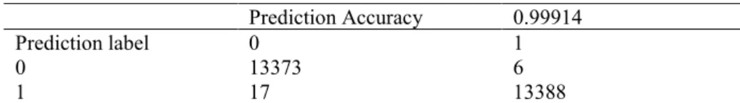
The result of using an SVC approach yielded a 99% accuracy. In subsequent phases, using dirtier data, closer to the raw data from the satellite, we believe the linearity of the data will not be as strong.

Table 2. Results from SVC analysis, demonstrating 99% accuracy

Prediction Accuracy 0.99914 Prediction label 0 1

0 13373 6

1 17 13388

5.2 Convolutional Neural Networks

Using a training and testing set of the data from the crustal field combined with the external field, the CNN has picked out the crustal field with 54.3% accuracy.

(13)

Table 3. Prediction table output from CNN.

Prediction Accuracy 54.3%

Prediction Label 0 1

0 521678 518725

1 147922 150875

In hindsight, this result is not too surprising. CNN's primary use is with large feature datasets for visual and text processing, neither of which we had. However, it does set the foundation of comparison in later phases of the project.

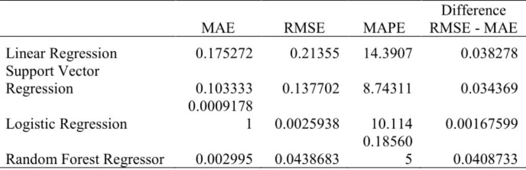
The Error Comparisons for Regression Approaches [25][26]. To evaluate the success of our model, we compare the following regression metrics for performance.

Table 4. Regression technique results for MAE, RMSE, and MAPE

MAE RMSE MAPE RMSE - MAE Difference Linear Regression 0.175272 0.21355 14.3907 0.038278 Support Vector

Regression 0.103333 0.137702 8.74311 0.034369

Logistic Regression 0.00091781 0.0025938 10.114 0.00167599 Random Forest Regressor 0.002995 0.0438683 0.185605 0.0408733

MAE. Using absolute numbers with no indication of the magnitude of the error, the Logistic Regression has the smallest MAE at .0009. The RFR also has a small MAE at .003. The largest MAE comes from Linear Regression at .175. The difference or distance between high to low MAE is .172.

RMSE. Looking at the impact and frequency of error, Logistic Regression is the smallest at .0025. RFR also has a small RMSE at .04.

The most significant difference between RMSE and MAE is .04 for Linear Regression and RFR, indicating larger distributions of error in these approaches. The smallest difference between MAE and RMSE is Logistic Regression with a difference of 0.001.

MAPE. Although considerable effort is made to create equality among the methods by using GridSearchCV, etc., the percentage comparison between approaches varies by 14.2%. Leading to greater model accuracy, by a noticeable amount, in the RFR at .186%. Logistic Regression and SVR are within 1.3% range of each other from 8.7-10%. Linear Regression has the highest model percentage error at 14%.

(14)

6 Conclusions and Recommendation

Given the reverse, iterative approach to finding the best machine learning method, it is not unexpected to receive the highly accurate results and the linearity of the dirty data (Crustal + External model). For Classification, the SVC outperformed the CNN due to the SVC’s and the data’s linear nature. From an approach perspective, and not a NASA productivity or efficiency needs perspective; a future attempt would take the Earth's magnetic image, as shown in Fig.4, and map that through a CNN. This approach more closely aligns to successful CNN attempts with visual images. The test would be for the ability of CNN to predict changes in the Earth’s magnetic crust based on the image, which results from raw satellite data.

For Phase 1 of our analysis, Linear Regression and SVR performed the least favorably in MAE and RMSE. These results are somewhat surprising given the linearity of the data. Logistic Regression and RFR have strengths in MAE and RMSE. RFR performed well across the board based on MAE, MAPE, and RMSE. Following phases of analyses will determine if RFR or Logistic Regression remain preferable approaches with dirtier data.

An adjacent approach is to ‘one-hot encode’ the data and maintain a history of magnetic data based on the spherical harmonics’ triangulation of the spot on the Earth. Then, with a sufficient dataset for each spot captured, use that data to predict the change in magnetism.

Phase 1’s foundation of regression and classification results create a solid foundation to find the optimum point of data condition by which machine learning is applied.

7 Ethics

Ethics in data collection, usage and retention are always important. The ethical considerations for this dataset and this paper are not significant. The Swarm data used falls under the ESA Data Policy for ERS, Envisat and Earth Explorer missions. The Policy's goal is to provide access in a nondiscriminatory way and allow the use of all primary and processed data (up to level 2) for scientific procedures, commercial practices, or for the public good [11]. Specifically, the ESA Data Policy is to encourage the following:

• continued Earth science activities;

• encourage technology innovation and instruments to observe the Earth;

• support operational applications and new applications being developed;

• support the private sector to invest in derived products and services;

• support global Earth Observation industry in the ESA Member States.

Since Swarm is part of the Earth mission, it is covered under the category of the policy outlining ‘Free dataset,' which includes full, and open, online access at no cost, abiding by the ESA terms and conditions. This dataset is also one-way, in which no data is uploaded to the ESA site. There is no private information in the dataset in which security needs must be taken into consideration. There are no ethical collection issues.

(15)

References

1. Sabaka, T.J. et al.: Extending comprehensive models of the Earths magnetic field with Ørsted and CHAMP data. Geophysical Journal International. 159, 2, 521–547 (2004).

2. Sabaka, T.J. et al.: CM5, a pre-Swarm comprehensive geomagnetic field model derived from over 12 yr of CHAMP, Ørsted, SAC-C and observatory data. Geophysical Journal International. 200, 3, 1596–1626 (2015).

3. Lesur, V. et al.: GRIMM: the GFZ Reference Internal Magnetic Model based on vector satellite and observatory data. Geophysical Journal International. 173, 2, 382–394 (2008). 4. Lesur, V. et al.: Parent magnetic field models for the IGRF-12GFZ-candidates. Earth, Planets and Space. 67, 1, (2015).

5. Olsen, N. et al.: LCS-1: a high-resolution global model of the lithospheric magnetic field derived from CHAMP and Swarm satellite observations. Geophysical Journal International. 211, 3, 1461–1477 (2017).

6. Lithospheric magnetic field,

http://www.esa.int/spaceinvideos/Videos/2017/03/Lithospheric_magnetic_field. 7. Maus, S. et al.: Resolution of direction of oceanic magnetic lineations by the sixth- generation lithospheric magnetic field model from CHAMP satellite magnetic measurements. Geochemistry, Geophysics, Geosystems. 9, 7, (2008).

8. Thébault, E. et al.: The satellite along-track analysis in planetary magnetism. Geophysical Journal International. 188, 3, 891–907 (2011).

9. Kotsiaros, S., Olsen, N.: The geomagnetic field gradient tensor. GEM - International Journal on Geomathematics. 3, 2, 297–314 (2012).

10. Random Forest vs Logistic Regression: Binary Classification for Heterogeneous Datasets, K. Kirasich, T. Smith, B. Sadler.

https://scholar.smu.edu/cgi/viewcontent.cgi?article=1041&context=datasciencereview 11. ESA Data Policy for ERS, Envisat and Earth Explorer missions, October 2012. https://earth.esa.int/c/document_library/get_file?folderId=296006&name=DLFE-3602.pdf 12. United Nations Resolution A/RES/41/65 dated 3 December 1986 on Principles relating to Remote Sensing of the Earth from Space.

13. Lithographic Magnetic Field. Richard Holm. https://www.liverpool.ac.uk/~holme/lith.html 15. Wikipedia - Lithosphere

https://en.wikipedia.org/wiki/Lithosphere. 15. Wikipedia – Subduction

https://en.wikipedia.org/wiki/Subduction.

(16)

https://earth.esa.int/web/guest/news/-/asset_publisher/G2mU/content/magnetic-lithosphere-detailed;jsessionid=0F5F7E6A634EB99B3912C9EC80BD0534.jvm1?redirect=https%3A%2F %2Fearth.esa.int%2Fweb%2Fguest%2Fnews%3Bjsessionid%3D0F5F7E6A634EB99B3912C9 EC80BD0534.jvm1%3Fp_p_id%3D101_INSTANCE_G2mU%26p_p_lifecycle%3D0%26p_p _state%3Dnormal%26p_p_mode%3Dview%26p_p_col_id%3Dcolumn-1%26p_p_col_pos%3D1%26p_p_col_count%3D2%26_101_INSTANCE_G2mU_cur%3D2% 26_101_INSTANCE_G2mU_keywords%3D%26_101_INSTANCE_G2mU_advancedSearch %3Dfalse%26_101_INSTANCE_G2mU_delta%3D10%26_101_INSTANCE_G2mU_andOper ator%3Dtrue

17. Thébault, Purucker, Whaler, Langlais, Sabaka : The Magnetic Field of the Earth’s

Lithosphere, Dec 2009.

18. Swarm, https://earth.esa.int/web/sppa/mission-performance/esa-missions/swarm 19. Finlay, C.C., Olsen, N., Kotsiaros, S., Gillet, N. and Toeffner-Clausen, L., (2016) Recent geomagnetic secular variation from Swarm and ground observatories as estimated in the CHAOS-6 geomagnetic field model. Earth, Planets, Space, 68, 112, doi: 10.1186/s40623-016-0486-1

20. Elagin, Andrey. (2018). Comparing Spherical Harmonics Analysis and Machine Learning Techniques for Double-Beta Decay Identification in a Large Liquid Scintillator Detector. Zenodo. http://doi.org/10.5281/zenodo.1345691

21. Wojciech Jarosz. Efficient Monte Carlo Methods for Light Transport in Scattering Media. Ph.D. dissertation, UC San Diego, September 2008.

https://cs.dartmouth.edu/wjarosz/publications/dissertation/appendixB.pdf

22. Leila Cristina C. Bergamasco, Carlos E. Rochitte, and Fátima L. S. Nunes. 2018. 3D medical objects processing and retrieval using Spherical Harmonics: a case study with Congestive Heart Failure MRI exams. In Proceedings of ACM SAC Conference, Pau,France, April 9-13, 2018 (SAC’18), 8 pages. DOI: 10.1145/3167132.3167168

23. Drew J., The Belk Endowment Educational Attainment Data Repository for North Carolina Public Schools, (2018), GitHub repository, https://github.com/jakemdrew/EducationDataNC 24. Turi Machine Learning Platform User Guide, https://turi.com/learn/userguide/supervised-learning/random_forest_regression.html.

25. Jj, Jj: MAE and RMSE - Which Metric is Better? – Human in a Machine World – Medium, https://medium.com/human-in-a-machine-world/mae-and-rmse-which-metric-is-better-e60ac3bde13d.

26. Using Mean Absolute Error to Forecast Accuracy, http://canworksmart.com/using-mean-absolute-error-forecast-accuracy/.

27. Botchkarev, Alexei. Performance Metrics (Error Measures) in Machine Learning Regression, Forecasting and Prognostics: Properties and Typology. Sep 2018. https://arxiv.org/pdf/1809.03006.pdf

(17)

28. Alvira Swalin.Choosing the Right Metric for Machine Learning Models.

https://medium.com/usf-msds/choosing-the-right-metric-for-machine-learning-models-part-1-a99d7d7414e4

29. Kotsiaros, S.: Toward more complete magnetic gradiometry with the Swarm mission. Earth, Planets and Space. 68, 1, (2016).

Appendix A

1. R Code

R version 3.5.1 (2018-07-02) -- "Feather Spray"

Platform: x86_64-w64-mingw32/x64 (64-bit)

R is free software and comes with ABSOLUTELY NO WARRANTY. You are welcome to redistribute it under certain conditions.

Type 'license()' or 'licence()' for distribution details. R is a collaborative project with many contributors. Type 'contributors()' for more information and

'citation()' on how to cite R or R packages in publications. Type 'demo()' for some demos, 'help()' for on-line help, or

'help.start()' for an HTML browser interface to help. Type 'q()' to quit R.

> # The header contained extra information. This was removed using WordPad. The file was originally save as a .dat file and so was converted to a .txt

> # The file is then read in as tab delimited file into a dataframe named data1

> setwd("C:/Users/Sheri/Documents/Data Science/Thesis/") > data1 <- read.delim(file="C:/Users/sheri/Documents/Data Science/Thesis/CHAOS_preds_SWC_20160101-20160131_mod.txt",header=FALSE, sep = '') > cran <- getOption("repos") > cran["dmlc"] <- "https://apache-mxnet.s3-accelerate.dualstack.amazonaws.com/R/CRAN/" > options(repos = cran) > install.packages("mxnet")

Installing package into ‘C:/Users/sheri/Documents/R/win

-library/3.5’

(18)

trying URL 'https://apache-mxnet.s3-accelerate.dualstack.amazonaws.com/R/CRAN/bin/windows/con trib/3.5/mxnet_1.3.0.zip'

Content type 'application/zip' length 30443134 bytes (29.0 MB)

downloaded 29.0 MB

package ‘mxnet’ successfully unpacked and MD5 sums checked

The downloaded binary packages are in

C:\Users\sheri\AppData\Local\Temp\Rtmp8mNdR9\downlo aded_packages

> require("mxnet")

Loading required package: mxnet > install.packages("mlbench")

-library/3.5’

(as ‘lib’ is unspecified)

trying URL

'https://cran.rstudio.com/bin/windows/contrib/3.5/mlbench _2.1-1.zip'

downloaded 1.0 MB

package ‘mlbench’ successfully unpacked and MD5 sums

checked

The downloaded binary packages are in

> library("mlbench") Warning message:

package ‘mlbench’ was built under R version 3.5.2 > install.packages("plot3D")

-library/3.5’

(as ‘lib’ is unspecified)

trying URL

'https://cran.rstudio.com/bin/windows/contrib/3.5/plot3D_ 1.1.1.zip'

downloaded 2.8 MB

package ‘plot3D’ successfully unpacked and MD5 sums checked The downloaded binary packages are in

(19)

> library("plot3D") Warning message:

package ‘plot3D’ was built under R version 3.5.2 > # Inspecting the data

> head(data1) V1 V2 V3 V4 V5 V6 V7 V8 V9 V10 V11 V12 V13 V14 1 5844 6833.886 162.8708 94.39791 45904.40 1960.22 -10062.76 45900.66 1958.78 -10066.81 3.73 1.44 4.05 53.51 2 5844 6833.887 162.9339 94.42800 45900.36 1986.93 -10060.42 45896.68 1985.38 -10064.46 3.68 1.55 4.05 53.52 3 5844 6833.888 162.9970 94.45834 45896.30 2013.66 -10058.01 45892.67 2012.00 -10062.05 3.63 1.66 4.04 53.53 4 5844 6833.889 163.0602 94.48893 45892.20 2040.43 -10055.54 45888.63 2038.65 -10059.58 3.56 1.77 4.04 53.54 5 5844 6833.891 163.1233 94.51977 45888.04 2067.22 -10053.01 45884.55 2065.34 -10057.03 3.50 1.88 4.03 53.55 6 5844 6833.892 163.1864 94.55087 45883.88 2094.04 -10050.41 45880.46 2092.06 -10054.43 3.42 1.98 4.01 53.56 V15 V16 V17 V18 V19 1 15.39 -4.41 45957.91 1975.62 -10067.17 2 15.28 -4.42 45953.88 2002.20 -10064.84 3 15.16 -4.43 45949.83 2028.82 -10062.44 4 15.04 -4.44 45945.74 2055.47 -10059.98 5 14.93 -4.45 45941.59 2082.15 -10057.45 6 14.81 -4.46 45937.44 2108.85 -10054.87 > tail(data1) V1 V2 V3 V4 V5 V6 V7 V8 V9 V10 V11 V12 2678395 5875 6834.278 170.7456 60.46576 40567.10 -2509.88 -12739.08 40569.44 -2508.29 -12739.39 -2.34 -1.59 2678396 5875 6834.279 170.8068 60.57665 40593.18 -2466.66 -12738.00 40595.49 -2465.03 -12738.28 -2.31 -1.63 2678397 5875 6834.280 170.8679 60.68907 40619.22 -2423.05 -12736.82 40621.50 -2421.38 -12737.08 -2.28 -1.67 2678398 5875 6834.281 170.9291 60.80305 40645.23 -2379.06 -12735.54 40647.48 -2377.35 -12735.79 -2.25 -1.71 2678399 5875 6834.282 170.9902 60.91861 40671.21 -2334.67 -12734.18 40673.43 -2332.92 -12734.40 -2.22 -1.75 2678400 5875 6834.283 171.0512 61.03580 40697.15 -2289.88 -12732.71 40699.34 -2288.09 -12732.91 -2.19 -1.79 V13 V14 V15 V16 V17 V18 V19 2678395 0.30 33.06 -1.87 -1.96 40600.16 -2511.76 -12741.05 2678396 0.28 33.06 -1.92 -1.98 40626.24 -2468.58 -12739.98 2678397 0.26 33.06 -1.97 -2.00 40652.28 -2425.02 -12738.82 2678398 0.24 33.06 -2.02 -2.02 40678.29 -2381.07 -12737.56

(20)

2678399 0.22 33.06 -2.06 -2.04 40704.27 -2336.73 -12736.22 2678400 0.20 33.06 -2.11 -2.06 40730.22 -2291.99 -12734.77 > summary(data1)

V1 V2 V3 V4 V5 V6

Min. :5844 Min. :6814 Min. : 2.648 Min. :-180.0000 Min. :-48793 Min. :-32958

1st Qu.:5852 1st Qu.:6820 1st Qu.: 45.169 1st Qu.: -90.2879 1st Qu.:-36730 1st Qu.:-22016

Median :5860 Median :6828 Median : 90.163 Median : -0.1035 Median : 2937 Median :-14929

Mean :5860 Mean :6826 Mean : 90.104 Mean : 0.2425 Mean : -981 Mean :-14734

3rd Qu.:5867 3rd Qu.:6833 3rd Qu.:135.064 3rd Qu.: 89.8413 3rd Qu.: 29694 3rd Qu.: -8611

Max. :5875 Max. :6835 Max. :177.352 Max. : 179.9995 Max. : 52931 Max. : 11531

V7 V8 V9 V10 V11

Min. :-12785.80 Min. :-48792 Min. :-32957 Min. :-12786.330 Min. :-15.34000

1st Qu.: -2939.43 1st Qu.:-36730 1st Qu.:-22016 1st Qu.: -2939.580 1st Qu.: -1.01000

Median : 90.12 Median : 2936 Median :-14929 Median : 89.770 Median : 0.01000

Mean : 1.64 Mean : -981 Mean :-14734 Mean : 1.638 Mean : 0.01122

3rd Qu.: 3166.59 3rd Qu.: 29695 3rd Qu.: -8612 3rd Qu.: 3166.815 3rd Qu.: 1.07000

Max. : 12282.23 Max. : 52934 Max. : 11528 Max. : 12281.600 Max. : 12.67000

V12 V13 V14 V15 V16

Min. :-7.73000 Min. :-10.620000 Min. :-55.1600 Min. :-12.39 Min. :-27.0000

1st Qu.:-0.69000 1st Qu.: -0.670000 1st Qu.:-18.3200 1st Qu.: 8.36 1st Qu.: -6.9925

Median : 0.07000 Median : -0.020000 Median : 0.0900 Median : 14.54 Median : 0.2300

Mean : 0.07041 Mean : 0.001557 Mean : -0.2081 Mean : 17.07 Mean : -0.1829

3rd Qu.: 0.85000 3rd Qu.: 0.610000 3rd Qu.: 17.8400 3rd Qu.: 22.39 3rd Qu.: 6.2500

Max. :11.38000 Max. : 7.830000 Max. : 54.9600 Max. :114.08 Max. : 24.6300

V17 V18 V19 Min. :-48824.1 Min. :-32952 Min. :-12793.780 1st Qu.:-36749.6 1st Qu.:-21992 1st Qu.: -2938.403

(21)

Median : 2937.3 Median :-14912 Median : 91.105 Mean : -981.2 Mean :-14716 Mean : 1.457 3rd Qu.: 29713.3 3rd Qu.: -8597 3rd Qu.: 3164.323 Max. : 52963.3 Max. : 11540 Max. : 12281.430 > ncol(data1) [1] 19 > nrow(data1) [1] 2678400 > any(is.na(data1)) [1] FALSE

> # So the columns represent the measurements from the five types of magnetometers

> # To do: Follow up with Stavros on which r, theta, phi group identifies with which magnetometer so we can label the columns appropriately

> data_header <- c("t","r","theta","phi","B_r1","B_theta1","B_phi1","B_r2" ,"B_theta2","B_phi2","B_r3","B_theta3","B_phi3","B_r4","B _theta4","B_phi4","B_r5","B_theta5","B_phi5") > colnames(data1) <- data_header > head(data1)

t r theta phi B_r1 B_theta1 B_phi1 B_r2 B_theta2 B_phi2 B_r3 B_theta3 B_phi3

1 5844 6833.886 162.8708 94.39791 45904.40 1960.22 -10062.76 45900.66 1958.78 -10066.81 3.73 1.44 4.05 2 5844 6833.887 162.9339 94.42800 45900.36 1986.93 -10060.42 45896.68 1985.38 -10064.46 3.68 1.55 4.05 3 5844 6833.888 162.9970 94.45834 45896.30 2013.66 -10058.01 45892.67 2012.00 -10062.05 3.63 1.66 4.04 4 5844 6833.889 163.0602 94.48893 45892.20 2040.43 -10055.54 45888.63 2038.65 -10059.58 3.56 1.77 4.04 5 5844 6833.891 163.1233 94.51977 45888.04 2067.22 -10053.01 45884.55 2065.34 -10057.03 3.50 1.88 4.03 6 5844 6833.892 163.1864 94.55087 45883.88 2094.04 -10050.41 45880.46 2092.06 -10054.43 3.42 1.98 4.01 B_r4 B_theta4 B_phi4 B_r5 B_theta5 B_phi5

1 53.51 15.39 -4.41 45957.91 1975.62 -10067.17 2 53.52 15.28 -4.42 45953.88 2002.20 -10064.84 3 53.53 15.16 -4.43 45949.83 2028.82 -10062.44 4 53.54 15.04 -4.44 45945.74 2055.47 -10059.98 5 53.55 14.93 -4.45 45941.59 2082.15 -10057.45 6 53.56 14.81 -4.46 45937.44 2108.85 -10054.87 > # Convolutional Neural Network

> # Create training and test datasets

> # source code:

https://stackoverflow.com/questions/17200114/how-to- split-data-into-training-testing-sets-using-sample-function

(22)

> ## 75% of the sample size

> smp_size <- floor(0.75 * nrow(data1))

> ## set the seed to make your partition reproducible > set.seed(123)

> train_ind <- sample(seq_len(nrow(data1)), size = smp_size) > train <- data1[train_ind, ] > test <- data1[-train_ind, ] > summary(train) t r theta phi B_r1 B_theta1

Min. :5844 Min. :6814 Min. : 2.648 Min. :-179.99999 Min. :-48793 Min. :-32958

1st Qu.:5852 1st Qu.:6820 1st Qu.: 45.096 1st Qu.: -90.24108 1st Qu.:-36775 1st Qu.:-22013

Median :5860 Median :6828 Median : 90.098 Median : -0.06814 Median : 2888 Median :-14928

Mean :5860 Mean :6826 Mean : 90.053 Mean : 0.25613 Mean : -1011 Mean :-14733

3rd Qu.:5867 3rd Qu.:6833 3rd Qu.:135.019 3rd Qu.: 89.81388 3rd Qu.: 29653 3rd Qu.: -8612

Max. :5875 Max. :6835 Max. :177.352 Max. : 179.99950 Max. : 52931 Max. : 11531

B_phi1 B_r2 B_theta2 B_phi2 B_r3

Min. :-12785.80 Min. :-48792 Min. :-32957 Min. :-12786.330 Min. :-15.34000

1st Qu.: -2941.46 1st Qu.:-36775 1st Qu.:-22013 1st Qu.: -2941.460 1st Qu.: -1.00000

Median : 89.31 Median : 2888 Median :-14927 Median : 89.020 Median : 0.02000

Mean : -0.29 Mean : -1011 Mean :-14733 Mean : -0.291 Mean : 0.01223

3rd Qu.: 3161.29 3rd Qu.: 29654 3rd Qu.: -8612 3rd Qu.: 3161.110 3rd Qu.: 1.07000

Max. : 12282.23 Max. : 52934 Max. : 11528 Max. : 12281.600 Max. : 12.67000

B_theta3 B_phi3 B_r4 B_theta4 B_phi4

(23)

B_r5 B_theta5 B_phi5 Min. :-48824 Min. :-32952 Min. :-12793.780 1st Qu.:-36794 1st Qu.:-21989 1st Qu.: -2940.325 Median : 2888 Median :-14911 Median : 90.330 Mean : -1011 Mean :-14716 Mean : -0.466 3rd Qu.: 29672 3rd Qu.: -8598 3rd Qu.: 3158.400 Max. : 52963 Max. : 11540 Max. : 12281.430 > summary(test)

t r theta phi B_r1 B_theta1

Min. :5844 Min. :6814 Min. : 2.648 Min. :-179.9996 Min. :-48792.1 Min. :-32958

1st Qu.:5852 1st Qu.:6820 1st Qu.: 45.383 1st Qu.: -90.4274 1st Qu.:-36595.9 1st Qu.:-22025

Median :5859 Median :6828 Median : 90.365 Median : -0.1717 Median : 3091.0 Median :-14933

Mean :5859 Mean :6826 Mean : 90.255 Mean : 0.2018 Mean : -891.5 Mean :-14736

3rd Qu.:5867 3rd Qu.:6833 3rd Qu.:135.201 3rd Qu.: 89.9404 3rd Qu.: 29811.1 3rd Qu.: -8609

Max. :5875 Max. :6835 Max. :177.352 Max. : 179.9989 Max. : 52931.3 Max. : 11531

B_phi1 B_r2 B_theta2 B_phi2 B_r3

Min. :-12785.780 Min. :-48791.3 Min. :-32957 Min. :-12786.300 Min. :-15.310000

1st Qu.: -2934.210 1st Qu.:-36595.6 1st Qu.:-22026 1st Qu.: -2934.445 1st Qu.: -1.010000

Median : 92.695 Median : 3090.9 Median :-14932 Median : 92.140 Median : 0.010000

Mean : 7.429 Mean : -891.5 Mean :-14736 Mean : 7.427 Mean : 0.008176

3rd Qu.: 3183.505 3rd Qu.: 29811.2 3rd Qu.: -8609 3rd Qu.: 3183.633 3rd Qu.: 1.070000

Max. : 12281.690 Max. : 52933.8 Max. : 11528 Max. : 12281.060 Max. : 12.650000

B_theta3 B_phi3 B_r4 B_theta4 B_phi4

(24)

B_r5 B_theta5 B_phi5 Min. :-48824.1 Min. :-32952 Min. :-12793.660 1st Qu.:-36616.1 1st Qu.:-22002 1st Qu.: -2933.012 Median : 3091.3 Median :-14916 Median : 93.355 Mean : -891.7 Mean :-14719 Mean : 7.227 3rd Qu.: 29831.0 3rd Qu.: -8595 3rd Qu.: 3180.102 Max. : 52963.2 Max. : 11540 Max. : 12278.980 > # removing negative values from the coordinates

> # Add the absolute value of the lowest x and y to shift the origin to the bottom left corner

> i <- min(train$phi) > j <- min(train$theta)

> train$phi <- train$phi + abs(i) > train$theta <- train$theta + abs(j) > # Creating initial plots

> # Using the B_r value to provide more variation in the plot and show more detail

> core_2D <- scatter2D(train$phi, train$theta, colvar = train$B_r2, col = ramp.col(c("blue", "yellow", "red"))) > crust_2D <- scatter2D(train$phi, train$theta, colvar = train$B_r3, col = ramp.col(c("blue", "yellow", "red"))) > ext_2D <- scatter2D(train$phi, train$theta, colvar = train$B_r4,col = ramp.col(c("blue", "yellow", "red"))) > # Separating the crustal field

> crust_train <- train[,c("t","r","theta","phi","B_r3","B_theta3","B_phi3" )] > crust_train$mag <- sqrt(crust_train$B_r3 * crust_train$B_r3 + crust_train$B_theta3 * crust_train$B_theta3 + crust_train$B_phi3 * crust_train$B_phi3) > crust_train$label <- 1

> c_train <- crust_train[,c("phi", "theta", "mag", "label")]

> head(c_train)

phi theta mag label 770248 101.7547 137.00533 0.7772387 1 2111396 104.8607 177.28091 2.9830354 1 1095403 172.9893 169.54833 2.6161231 1 2365072 272.8674 121.94003 5.0093313 1 2518944 165.6680 29.88937 5.2148058 1 122019 114.2449 68.62554 1.5667163 1

(25)

> nrow(c_train) [1] 2008800

> crust_test <-

test[,c("t","r","theta","phi","B_r3","B_theta3","B_phi3") ]

> crust_test$mag <- sqrt(crust_test$B_r3 * crust_test$B_r3

+ crust_test$B_theta3 * crust_test$B_theta3 +

crust_test$B_phi3 * crust_test$B_phi3) > crust_test$label <- 1

> c_test <- crust_test[,c("phi", "theta", "mag", "label")] > head(c_test)

phi theta mag label 10 94.67786 163.4388 5.538447 1 16 94.87651 163.8172 5.320357 1 18 94.94501 163.9433 5.227332 1 19 94.97970 164.0063 5.181477 1 29 95.34367 164.6362 4.650387 1 32 95.45927 164.8250 4.489822 1 > nrow(c_test) [1] 669600

> # Separating the external field

> external_train <- train[,c("t","r","theta","phi","B_r4","B_theta4","B_phi4" )] > external_train$mag <- sqrt(external_train$B_r4 * external_train$B_r4 + external_train$B_theta4 * external_train$B_theta4 + external_train$B_phi4 * external_train$B_phi4) > external_train$label <- 0

> e_train <- external_train[,c("phi", "theta", "mag", "label")]

> head(e_train)

phi theta mag label 770248 101.7547 137.00533 17.46832 0 2111396 104.8607 177.28091 26.42282 0 1095403 172.9893 169.54833 29.87461 0 2365072 272.8674 121.94003 24.36782 0 2518944 165.6680 29.88937 22.51942 0 122019 114.2449 68.62554 30.99013 0 > nrow(e_train) [1] 2008800 > external_test <- test[,c("t","r","theta","phi","B_r4","B_theta4","B_phi4") ] > external_test$mag <- sqrt(external_test$B_r4 * external_test$B_r4 + external_test$B_theta4 * external_test$B_theta4 + external_test$B_phi4 * external_test$B_phi4)

(26)

> external_test$label <- 0

> e_test <- external_test[,c("phi", "theta", "mag", "label")]

> head(e_test)

phi theta mag label 10 94.67786 163.4388 55.66985 0 16 94.87651 163.8172 55.54672 0 18 94.94501 163.9433 55.51164 0 19 94.97970 164.0063 55.48357 0 29 95.34367 164.6362 55.31372 0 32 95.45927 164.8250 55.26211 0 > nrow(e_test) [1] 669600

> # Combining the external and crustal field to provide a realistic dataset in which to search for the crustal field > # Also normalizing the data for more clarity in the CNN run

> combined_train <- rbind(c_train, e_train) > com_train_scaled <- combined_train

> com_train_scaled$mag <- scale(combined_train$mag) > head(com_train_scaled)

phi theta mag label 770248 101.7547 137.00533 -0.9489097 1 2111396 104.8607 177.28091 -0.8035846 1 1095403 172.9893 169.54833 -0.8277580 1 2365072 272.8674 121.94003 -0.6700856 1 2518944 165.6680 29.88937 -0.6565482 1 122019 114.2449 68.62554 -0.8968963 1 > nrow(com_train_scaled) [1] 4017600

> combined_test <- rbind(c_test, e_test) > com_test_scaled <- combined_test

> com_test_scaled$mag <- scale(combined_test$mag) > head(com_test_scaled)

phi theta mag label 10 94.67786 163.4388 -0.6353813 1 16 94.87651 163.8172 -0.6497494 1 18 94.94501 163.9433 -0.6558781 1 19 94.97970 164.0063 -0.6588991 1 29 95.34367 164.6362 -0.6938882 1 32 95.45927 164.8250 -0.7044665 1 > nrow(com_test_scaled) [1] 1339200 > dim(com_train_scaled) [1] 4017600 4 > train.x <- data.matrix(com_train_scaled[,1:3]) > train.y <- com_train_scaled[,4] > mx.set.seed(0)

(27)

> model <- mx.mlp(train.x, train.y, hidden_node=5, out_node=2, out_activation="softmax", + num.round=5, array.batch.size=15, learning.rate=0.07, momentum=0.9, + eval.metric=mx.metric.accuracy, array.layout = "rowmajor")

Start training with 1 devices

[1] Train-accuracy=0.499977364318179 [2] Train-accuracy=0.499971639507076 [3] Train-accuracy=0.499971639507076 [4] Train-accuracy=0.499971639507076 [5] Train-accuracy=0.499971639507076 > test.x <- data.matrix(combined_test[,1:3]) > test.y <- combined_test[,4]

> preds = predict(model, test.x) Warning message:

In mx.model.select.layout.predict(X, model) :

Auto detect layout of input matrix, use rowmajor.. > sqrt(mean((preds-test.y)^2)) [1] 0.54394 > pred.label = max.col(t(preds))-1 > table(pred.label, test.y) test.y pred.label 0 1 0 521678 518725 1 147922 150875

2. Python Code

# coding: utf-8

# Code from Dr Jake Drew, SMU #

https://github.com/jakemdrew/EducationDataNC/blob/master/ 2017/Models/2017GraduationRates4yr.ipynb

#and SMU Data Mining Class

# ## Data Setup - r, theta, phi, magnitude # In[2]:

import pandas as pd import numpy as np

df_trainSM = pd.read_csv('/Users/laurabishop/Documents/R Repositories/Capstone Magnetic Field/combined_all_SM.csv')

(28)

df_trainSM.columns = ['Unnamed','theta','phi', 'mag', 'label']

df_trainSM = df_trainSM.drop('Unnamed', 1) print("Training data for small data frame") print ('Size of the dataset:', df_trainSM.shape)

print ('Information about dataset: ', df_trainSM.info()) print ('Head: ', df_trainSM.head())

# ## Data Exploration - r, theta, phi, magnitude # In[2]: import matplotlib.pyplot as plt plt.plot(df_trainSM) plt.show() # In[3]: plt.plot(df_trainSM) plt.savefig('rThetaPhiMagPLOT.pdf', orientation='portrait', papertype='letter') plt.close() # In[4]:

#From SMU Data Mining Class import seaborn as sns import matplotlib.pyplot as plt #sns.pairplot(df_testSM, vars=['B_r3', # 'B_theta3', # 'B_phi3'], hue='B_r3') sns.pairplot(df_trainSM)

#plt.title ('Pair Plot for External Training Split') plt.show() # In[5]: sns.pairplot(df_trainSM) plt.savefig('rThetaPhiMagPAIRPLOT.pdf', orientation='portrait', papertype='letter') plt.close() # In[22]:

(29)

#From SMU Data Mining Class #theta & phi

import matplotlib.pyplot as plt N=50

#mag & phi

y = np.array (df_trainSM.mag) x = np.array (df_trainSM.phi)

area = np.pi * (3 * np.random.rand(N))**2 # 0 to 3 point radii

plt.scatter(x, y, color='g', s=5, linewidths=0, alpha=0.5) plt.title('Scatter for mag compared to phi')

plt.show() #mag and theta

y = np.array (df_trainSM.mag) x = np.array (df_trainSM.theta)

area = np.pi * (3 * np.random.rand(N))**2 # 0 to 3 point radii

plt.scatter(x, y, color='r', s=5, linewidths=0, alpha=0.5) plt.title('Scatter for mag compared to theta')

plt.show()

# In[5]:

#From SMU Data Mining Class #theta & phi

import numpy as np import pandas as pd import matplotlib.pyplot as plt N=50 x = [] y = [] for i in range(len(df_trainSM)) : if df_trainSM.label[i] == 0: x.append(i) else: y.append(i) for j in range (13379,13405): x.append(j) == np.nan df = pd.DataFrame({'x':x, 'y':y}) df.columns = ['External', 'Crustal']

df.plot(kind='scatter',x='External',y='Crustal', color='red')

(30)

plt.show()

plt.scatter(x, y, color='g', s=5, linewidths=0, alpha=0.5) plt.title('Scatter Crustal Field Data v External Field Data')

plt.xlabel("External Field Data (Noise) - Number of Rows") plt.ylabel("Crustal Field Data - Number of Rows")

plt.savefig('PLOTExternalCrustal.pdf', orientation='portrait', papertype='letter') plt.close() plt.show() # In[56]: print (np.shape(x)) print (np.shape(y)) print (type(x)) #for i in range(len(x)) : # if x[i] == 0 or x[i] == 1: # print("hi") # else: # print (i) #x[i] == np.nan print (np.shape(x))

# ## Create Linear Regression Variables # In[6]:

# create x explanatory and y response variables for regression DATAFRAME

#Y_bt3 = df_trainSM['B_theta3'] #Y_BP3 = df_trainSM['B_phi3'] Ylabel = df_trainSM['label'] if 'label' in df_trainSM:

yMagVal = df_trainSM['label'].values # get the values we want

#del df_trainSM['label'] # get rid of the class label X = df_trainSM.values # use everything else to predict! #already done in if statement above

X_Comb = df_trainSM.drop('label', axis=1) Y = Ylabel

#inspect data X_Comb.info() # In[ ]:

(31)

X_Comb

# ## PREPROCESSING # In[7]:

###PREPROCESSING

from sklearn import preprocessing from decimal import Decimal

X_CombScale = preprocessing.scale(X_Comb) min_max_scaler = preprocessing.MinMaxScaler()

np_scaled = min_max_scaler.fit_transform(X_CombScale) X_CombPre = pd.DataFrame(X_CombScale)

X_CombPre.columns = ['theta','phi', 'mag'] X_CombPre['phi'] = round (X_CombPre['phi'], 2) X_CombPre['theta'] = round (X_CombPre['theta'], 2) X_CombPre['mag'] = round (X_CombPre['mag'], 2) X_CombPre

# # Split Training Data #

# In[8]:

#Divide data into test and training splits

from sklearn.model_selection import ShuffleSplit

cv = ShuffleSplit(n_splits=5, test_size=0.20,

random_state=0)

# ## DataFrame to Store Regression Results # In[9]:

colList = ['MAE','MAPE','RMSE']

dfResult = pd.DataFrame(columns= colList) dfResult

# # 4.3 Machine Learning -- map to the Capstone paper section.

# This paper examines five (5) machine learning approaches to see which method best

# predicts the data useful for the crustal data model. The approach taken is inverse data analysis. Instead of starting

# at the beginning with dirtiest data straight from the satellite, struggling with cleaning and clustering,

(32)

# and wondering if

# errors or challenges are due to the premise or a challenge in the data; we start with clean known to work data (crustal model) that is

# mixed with other external model data to create first phase 'dirty data set'. If the crustal model data can be # successfully predicted amongst the external model data, success is achieved at Phase 1. The next step is to use the data set in a dirtier, earlier revision from the satellite. The

# number of backward iterations is not known at this time, but estimated to be at least four (4) will be required to # confidently know this approach is statistically successful and useable by NASA Goddard.

#

# Additionally, this paper does not delve into the fuzzy barrier between machine learning and

# statistical learning. Given all learning is done from the data, the approaches are classified as machine learning.

#

# For each approach the measure of a good machine learning technique is its

# error rate. In order to evaluate the approaches, three (3) error measures are used to evaluate the distance between estimates and predictions:

# 1. Mean Absolute Error (MAE) - Smaller error is better. Less sensitive to outliers and easy to use.

# 2. Root mean Squre Error (RMSE) - Shows absolute fit of the model.

# 3. Mean Absolute Percentage Error (MAPE) - Small relative error and shows precision of the models.

# <footnote: approach and code from Code from Dr Jake Drew,

Southern Methodist University

https://github.com/jakemdrew/EducationDataNC/blob/master/ 2017/Models/2017GraduationRates4yr.ipynb >

# The model analysis code use was built by Dr. Jacob Drew of Southern Methodist University and his work for the State of North Carolina Education. <footnote: Ibid.>

#

# The model analysis code builds regression models that are evaluated using cross validation and a random seed. This

is accomplished using parameters of Python's

sklearn.model_selection's cross_validate function, which performs the cross validation for

# regression estimators. The random seed ensures that all regression

(33)

# the same randomly selected data rows for each cross validation fold. Drew created custom scorers for MAE, RMSE, and MAPE using the three

# chosen mean error scores. Thus all three scores are calcualted using a single call

# to cross_validate(). All of this functionality lies in a custom function 'EvaluateRegressionEstimator()', which allows multiple regression models to be tested using the same test / train cv data and produces the

# evaluation scores in a consistent manner for each model. <footnote: Ibid>

#

# For these approaches, a sample size of the 2.6 million SWARM satellite data was used totalling 26,784 rows and five (5) folds. The training set is 21,427 rows and test set is 5,357 rows.

# Reference:

# Drew J., The Belk Endowment Educational Attainment Data Repository for North Carolina Public Schools, (2018),

GitHub repository, https://github.com/jakemdrew/EducationDataNC # https://www.quora.com/Why-we-use-Root-mean-square- error-RMSE-Mean-absolute-and-mean-absolute-percent-errors-for-forecasting-time-series-models # MAPE. https://en.wikipedia.org/wiki/Mean_absolute_percentage_er ror # MAE. https://en.wikipedia.org/wiki/Mean_absolute_error # RMSE. https://www.theanalysisfactor.com/assessing-the-fit-of-regression-models/ # In[10]:

Dr Jake Drew code SMU

#Use mean absolute error (MAE) to score the regression models created

#(the scale of MAE is identical to the response variable)

from sklearn.metrics import mean_absolute_error,

make_scorer, mean_squared_error

#Function for Root mean squared error

#https://stackoverflow.com/questions/17197492/root-mean-square-error-in-python

(34)

def rmse(y_actual, y_predicted):

return np.sqrt(mean_squared_error(y_actual,

y_predicted))

#Function for Mean Absolute Percentage Error (MAPE) - Untested

#Adapted from -

https://stackoverflow.com/questions/42250958/how-to-optimize-mape-code-in-python

def mape(y_actual, y_predicted): mask = y_actual != 0

return (np.fabs(y_actual -

y_predicted)/y_actual)[mask].mean() * 100 #Create scorers for rmse and mape functions

mae_scorer = make_scorer(score_func=mean_absolute_error, greater_is_better=False) rmse_scorer = make_scorer(score_func=rmse, greater_is_better=False) mape_scorer = make_scorer(score_func=mape, greater_is_better=False)

#Make scorer array to pass into cross_validate() function for producing mutiple scores for each cv fold.

errorScoring = {'MAE': mae_scorer, 'RMSE': rmse_scorer, 'MAPE': mape_scorer }

# In[11]:

from sklearn.model_selection import cross_validate

def EvaluateRegressionEstimator(regEstimator, X, y, cv):

scores = cross_validate(regEstimator, X, y,

scoring=errorScoring, cv=cv, return_train_score=True) #cross val score sign-flips the outputs of MAE

https://github.com/scikit-learn/scikit-learn/issues/2439

scores['test_MAE'] = scores['test_MAE'] * -1 scores['test_MAPE'] = scores['test_MAPE'] * -1 scores['test_RMSE'] = scores['test_RMSE'] * -1 #print mean MAE for all folds

maeAvg = scores['test_MAE'].mean()

print_str = "The average MAE for all cv folds is: \t\t\t {maeAvg:.5}"

print(print_str.format(maeAvg=maeAvg)) #print mean test_MAPE for all folds

(35)

scores['test_MAPE'] = scores['test_MAPE'] mape_avg = scores['test_MAPE'].mean()

print_str = "The average MAE percentage (MAPE) for all cv folds is: \t {mape_avg:.5}"

print(print_str.format(mape_avg=mape_avg)) #print mean MAE for all folds

RMSEavg = scores['test_RMSE'].mean()

print_str = "The average RMSE for all cv folds is: \t\t\t {RMSEavg:.5}"

print(print_str.format(RMSEavg=RMSEavg))

print('************************************************** *******')

print('Cross Validation Fold Mean Error Scores') scoresResults = pd.DataFrame()

scoresResults['MAE'] = scores['test_MAE'] scoresResults['MAPE'] = scores['test_MAPE'] scoresResults['RMSE'] = scores['test_RMSE'] return scoresResults

# # Creates the comparison dataframe for the different methods.

# In[12]:

#this is to gather RMSE MAPE MAE to put into a table that shows the result based on approach.

#The goal is to make comparison easier def ERE(regEstimator, X, y, cv):

scores = cross_validate(regEstimator, X, y,

scoring=errorScoring, cv=cv, return_train_score=True) #cross val score sign-flips the outputs of MAE

#

https://github.com/scikit-learn/scikit-learn/issues/2439

scores['test_MAE'] = scores['test_MAE'] * -1 scores['test_MAPE'] = scores['test_MAPE'] * -1 scores['test_RMSE'] = scores['test_RMSE'] * -1 #print mean MAE for all folds

maeAvg = scores['test_MAE'].mean()

#print_str = "The average MAE for all cv folds is: \t\t\t {maeAvg:.5}"

#print(print_str.format(maeAvg=maeAvg)) #print mean test_MAPE for all folds

scores['test_MAPE'] = scores['test_MAPE'] mape_avg = scores['test_MAPE'].mean()