How to Project Customer Retention
Peter S. Fader
Bruce G. S. Hardie1
May 2006
1Peter S. Fader is the Frances and Pei-Yuan Chia Professor of Marketing at the Wharton School of the University of Pennsylvania (address: 749 Huntsman Hall, 3730 Walnut Street, Philadelphia, PA 19104-6340; phone: 215.898.1132; email: [email protected]; web: www.petefader.com). Bruce G. S. Hardie is Associate Professor of Marketing, London Business School (email: [email protected]; web: www.brucehardie.com). The authors thank Michael Berry and Gordon Linoff for providing the data used in this paper, and Naufel Vilcassim for his helpful comments. The second author acknowledges the support of the London Business School Centre for Marketing and the hospitality of the Department of Marketing at the University of Auckland Business School.
Abstract
How to Project Customer Retention
At the heart of any contractual or subscription-oriented business model is the notion of the retention rate. An important managerial task is to take a series of past retention numbers for a given group of customers and project them into the future in order to make more accurate predictions about customer tenure, lifetime value, and so on. In this paper we reanalyze data from a leading book on data mining (Berry and Linoff 2004), who drew the dire conclusion that “parametric approaches do not work” for such a task. As an alternative to common “curve-fitting” regression models, we develop and demonstrate a probability model with a well-grounded “story” for the churn process. We show that our basic model (known as a “shifted-beta-geometric”) can be implemented in a simple Microsoft Excel spreadsheet and provides remarkably accurate forecasts and other useful diagnostics about customer retention. We provide a detailed appendix covering the implementation details and offer additional pointers to other related models.
Keywords: retention, churn, forecasting, customer base analysis, probability models, beta-geometric
1 Introduction
A defining characteristic of a contractual or subscription business setting is that the departure of a customer is observed. For example, the customer has to contact the firm to cancel her mobile phone contract; similarly, a local theater company can observe that a patron has not renewed his annual subscription.1 As such, it makes sense to talk of metrics such as retention and churn rates: the retention rate for periodt(rt) is defined as the proportion of customers active at the end of period t−1 who are still active at the end of periodt, while the churn rate for a given period is defined as the proportion of customers active at the end of period t−1 who dropped out in periodt.2
As we seek to understand the nature of customer behavior in a contractual setting, it is useful to draw on the survival analysis literature. One particularly useful concept for characterizing the distribution of customer lifetimes is that of thesurvivor function, denoted byS(t), which is the probability that a customer has “survived” to timet (i.e., is still active att). Recalling the definition of a retention rate, it follows that
S(t) =r1×r2× · · · ×rt =t i=1 ri, (1) which implies rt= S(St(−t)1). (2)
Several quantities of managerial interest can easily be calculated directly from the survivor function. For example, the expected (or average) tenure of a customer is simply the area under the survivor function. In a discrete-time setting, this is computed as
expected tenure = ∞
t=0
S(t).
In light of (1), the standard textbook expression for (expected) customer lifetime value (CLV)
1This is in contrast to a noncontractual setting, a defining characteristic of which is that the departure of a
customer is not observed by the firm. See Section 4.1 for a discussion of the implications of this characteristic.
in a contractual setting that (correctly) reflects the phenomenon of nonconstant retention rates, E(CLV) = ∞ t=0 m t i=1 ri 1 1 +d t , can be written as E(CLV) =∞ t=0 m(1 +S(td))t.
In a contractual setting, the empirical survivor function S(t) is simply the proportion of customers acquired at time 0 who are still active at time t. A major problem in using the empirical survivor function to compute expected tenure or lifetime value is that the observed time horizon is often quite limited. Suppose we observe a particular cohort of customers over their first five years with the firm, which implies we can compute S(1), . . .S(5). (By definition,
S(0) = 1.) The quantity S(0) +· · ·+S(5) is the expected customer lifetime for the members of the cohort over this period. Similarly, we can compute expected CLV during the first five years of a customer’s relationship with the firm. However, we would be underestimatimg the expected tenure and CLV of a new customer as we would be ignoring the remaining life of those customers who are alive at the end of the fifth year. In order to compute the true expected tenure and CLV, we need to be able to project the survivor function beyond the observed time horizon. That is, we need to create estimates ofS(6), S(7), . . .given the dataS(1), . . .S(5). This projected survivor function is also needed if we wish to compute the expected residual tenure or lifetime value of an individual who has been a customer for, say, three years.
An obvious approach is to fit some flexible function of time to the observed data. The resulting regression equation can then be used to project the survivor function beyond the range of observations, from which we can compute expected tenure, customer lifetime value, etc. In a popular book on data mining, Berry and Linoff (2004) explore this idea (on pages 392–393); their conclusion regarding the viability of such an exercise is evident in the title of their sidebar discussion: “Parametric approaches do not work”.
The objective of this paper is to present an alternative approach to the problem of projecting the survivor function, one that does “work”. We formulate a probabilistic model of contract duration that is based on a simple story of customer behavior. The resulting model offers useful
diagnostic insights and is very easy to implement using Microsoft Excel.
In the next section, we replicate and extend Berry and Linoff’s analysis. We then present a simple probability model of customer lifetime and demonstrate the value of using a formal model to predict future customer behavior. We conclude with a discussion of several issues that arise from this work.
2 Projecting Survival Using Simple Functions of Time
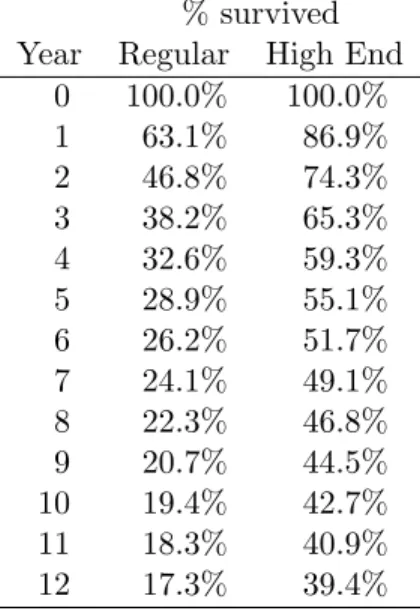
The survival data presented in Table 1 are for two segments of customers (“Regular” and “High End”) for an unspecified subscription-type business. These data are presented in graphical form in Berry and Linoff (2004, Chapter 12). The High End data are used by Berry and Linoff in their examination of parametric approaches to the projection of the survivor function.
% survived Year Regular High End
0 100.0% 100.0% 1 63.1% 86.9% 2 4 6.8% 74.3% 3 38.2% 65.3% 432.6% 59.3% 5 28.9% 55.1% 6 26.2% 51.7% 7 24.1% 49.1% 8 22.3% 46.8% 9 20.7% 44.5% 10 19.4 % 4 2.7% 11 18.3% 40.9% 12 17.3% 39.4%
Table 1: Observed % customers surviving at least 0–12 years
Suppose we only have the first seven years of data and wish to compute estimates of
S(8), S(9), . . .. If we were to give these data to a student who had just completed a typical data analysis course, the natural starting point would be to fit a linear function of time to the data and use the resulting regression equation to project the survivor function out over the future periods. Recognizing that the data are not linear, some students would add a quadratic term to try to capture the curvature in the data. More sophisticated students would specify
some nonlinear function of time, such as an exponential function.
In their “Parametric approaches do not work” sidebar, Berry and Linoff estimate and com-pare this set of regression models with the following results:3
Linear y= 0.925−0.071t R2 = 0.922 Quadratic y= 0.997−0.142t+ 0.010t2 R2 = 0.998 Exponential ln(y) =−0.062−0.102t R2 = 0.963
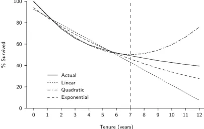
whereyis the proportion of customers surviving at leasttyears. These equations are then used to extrapolate the survivor function out to year 12; Figure 1 re-creates the plot presented in Berry and Linoff’s sidebar (p. 393).
0 1 2 3 4 5 6 7 8 9 10 11 12 Tenure (years) 0 20 40 60 80 100 % Survived ...... ...... ...... ...... ...... ...... ...... Actual ...... ...... ...... ...... ...... ...... ...... ...... ...... ...... ... Linear ... ... ... ... ...... ... ...... ...... ... ... ... ... Quadratic ... ... ... ...... ...... ... ... ... ... ... ... ... ... ... ...... ... ... ... ... ...... ... ... ... ... ... ... ... Exponential
Figure 1: Actual versus model-based estimates of the percentage of High End customers surviving at least 0–12 years
The fit of all three models up to and including year 7 is reasonable, and the quadratic model provides a particularly good fit. But when we consider the projections beyond the model cali-bration period, all three models break down dramatically. The linear and exponential models underestimate year 12 survival by 81% and 30%, respectively, while the quadratic model over-estimates year 12 survival by 92%. Furthermore, the models lack logical consistency: the linear model would haveS(t)<0 after year 14, and according to the quadratic model the survival will
3In the models run by Berry and Linoff, time is indexed 1,2, . . . ,8, but in order to maintain consistency with
the definitions ofS(t) discussed earlier (specificallyS(t) = 0), we reindex time to 0,1, . . . ,7. This has no impact at all on the fit or forecasting performance of any of the models.
start to increase over time, which is not possible. It is therefore not surprising that Berry and Linoff conclude that parametric curves do not “work” for the task of projecting the survivor function over time.
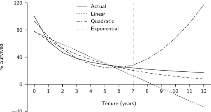
Repeating this analysis for the Regular segment yields the following equations: Linear y= 0.773−0.092t R2 = 0.776 Quadratic y= 0.930−0.249t+ 0.022t2 R2 = 0.960 Exponential ln(y) =−0.248−0.190t R2 = 0.915
and the corresponding fits and projections are reported in Figure 2. The projections associated with the linear and quadratic models are terrible and illogical once again. The exponential model doesn’t appear to be very bad in the figure, but in fact it underestimates year 12 survival by 54%. This is not an acceptable range of error.
0 1 2 3 4 5 6 7 8 9 10 11 12 Tenure (years) −40 0 40 80 120 % Survived ...... ...... ...... ...... ...... ...... Actual ...... ...... ...... ... ...... ...... ...... ...... ... Linear ... ... ...... ... ...... ...... ... ... ... ... ... ... ... ... ... Quadratic ...... ... ... ... ... ... ...... ... ... ... ... ...... ... ... ... ... ... ... ... ... ...... ... ... ... ... ... ... ... ... Exponential
Figure 2: Actual versus model-based estimates of the percentage of Regular customers surviving at least 0–12 years
Of course we could try out different arbitrary functions of time but this would be a pure curve-fitting exercise at its worst. Furthermore, it is hard to imagine that there would any underlying rationale for the equation(s) that we might settle upon. Faced with this situation, it is tempting to throw up our hands in despair and say that we cannot project out the survivor function beyond the range of observations.
However, we feel that such a conclusion is premature. After all, in other areas of marketing there are plenty of models that have been used to provide accurate forecasts of the behavior of
a cohort of customers beyond the range of observations (see, for instance, Hardie, Fader and Wisniewski (1998) for the case of new product sales forecasting) . With this in mind, the next section sees us formulating a probabilistic model of contract duration that is based on a simple “story” of customer behavior.
3 ADiscrete-Time Model for Contract Duration
Consider the following story of customer behavior in a contractual setting:
i. At the end of each period, a customer flips a coin: “heads” she cancels her contract, “tails” she renews it.
ii. For a given individual, the probability of a coin coming ups “heads” does not change over time.
iii. P(“heads”) varies across customers.
Of course people do not make their contract renewal decisions on the basis of coin flips; rather, this story is a paramorphic representation of customer behavior. The third element of the story should be not be controversial, as the notion of heterogeneity is central to marketing. However, some readers might find the second element contrary to their expectation that retention rates increase over time as the customer gains more experience with the product or service. But rather than overcomplicate our story, we start with the simplest possible set of assumptions and only add supposed richer “touches of reality” if the model does not “work”. As we will see shortly, no additional assumptions will be required in this particular case.
To operationalize this verbal model, we need to translate the elements of this story into the language of mathematics. More formally, our proposed model for the duration of customer lifetimes is based on the following two assumptions:
i. An individual remains a customer of the firm with constant retention probability 1−θ. This is equivalent to assuming that the duration of the customer’s relationship with the firm, denoted by the random variableT, is characterized by the (shifted) geometric distribution
with probability mass function and survivor function
P(T =t|θ) =θ(1−θ)t−1, t= 1,2,3, . . . (3)
S(t|θ) = (1−θ)t, t= 1,2,3, . . . (4)
ii. Heterogeneity inθ follows a beta distribution with pdf
f(θ|α, β) =θα−1(1−θ)β−1
B(α, β) , whereB(·,·) is the beta function.
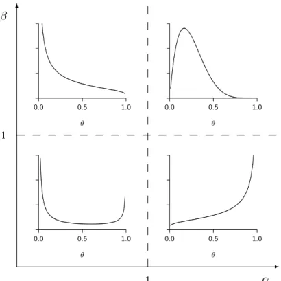
The assumption of geometrically-distributed lifetimes follows from the first two elements of our simple story of customer behavior; it is perfectly consistent with the sequential coin-flip description. The beta distribution is less familiar to most readers, but it is a very reasonable way to characterize heterogeneity in the churn probabilities because it is a flexible distribution which is bounded between zero and one. If one thinks about how the “coin-flip” probabilities are likely to vary across individuals, there are four principal possibilities, as illustrated in Figure 3. If both parameters of the beta distribution (α and β) are small (less than 1), then the mix of churn probabilities is “U-shaped,” or highly polarized across customers. If both parameters are relatively large (α, β > 1), then the probabilities are fairly homogeneous. Likewise, the distribution of probabilities can be “J-shaped” or “reverse-J-shaped” if the parameters fall within the remaining ranges as shown in the figure. It is not essential for the reader to remember all of these cases, but these parameters can offer useful diagnostics to help the manager understand the degree (and nature) of heterogeneity in churn probabilities across the customer base.
Given these two model assumptions, how can we compute the probability that a customer fails to renew his contract at the end of thetth period or survives beyond periodt(P(T =t) and
S(t) respectively)? Since this customer’s value of θ is unobserved, we cannot use (3) and (4). We therefore take the expectation of (3) and (4) over the beta distribution that characterizes the cross-sectional heterogeneity inθto arrive at the corresponding expressions for a randomly-chosen individual:
✲ ✻ α β 1 1 0.0 0.5 1.0 θ ...... ... ...... ...... ...... ... ... ... 0.0 0.5 1.0 θ ...... ...... ...... ... ...... ...... 0.0 0.5 1.0 θ ... ... ... ... ... ... ... ... . 0.0 0.5 1.0 θ ... ... ... ... ... ... ... ...... ...... ...... ... ...... ...
Figure 3: General shapes of the beta distribution as a function of α and β
P(T =t|α, β) = B(α+ 1B(, βα, β+)t−1), t= 1,2, . . . (5)
S(t|α, β) = BB(α, β(α, β+)t), t= 1,2, . . . (6) (The mathematically-inclined reader is referred to Appendix A for step-by-step details of the derivations.) We call this model the shifted-beta-geometric (sBG) distribution. Non-business applications of this model include the number of menstrual cycles required to achieve pregnancy (Weinberg and Gladen 1986) and lengths of stay in a psychiatric hospital (Kaplan 1982). Direct marketing applications of related models are discussed in Section 4.
It turns out that we can use this model without ever having to deal with a beta function. As formally derived in Appendix A, we can compute sBG probabilities by using the following forward-recursion formula fromP(T = 1):
P(T =t) = α α+β t= 1 β+t−2 α+β+t−1P(T =t−1) t= 2,3, . . . (7)
Recall from (2) that the retention rate is the ratio of sequential values of the survivor function. Substituting (6) into (2) and simplifying (see Appendix A) gives us the following expression for the (aggregate) retention rate associated with sBG model:
rt= α+β+β+t−t−1 1. (8)
Given (8), we can go back to the expression given in (1) and compute S(t) without having to deal with any beta functions.
We immediately see that, under the sBG model, the retention rate is an increasing function of time, even though the underlying (unobserved) individual-level retention probability is constant. According to this model, there are no underlying time dynamics at the level of the individual customer; the observed phenomenon of retention rates increasing over time is simply due to heterogeneity (i.e., the high churn customers drop out early in the observation period, with the remaining customers having lower churn probabilities). This well-known “ruse of heterogeneity” (Vaupel and Yashin 1985) is often overlooked by those attempting to make sense of various aggregate patterns of customer behavior.
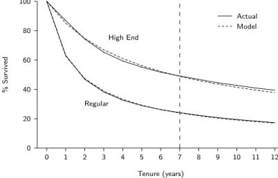
We fit the sBG model to the first seven years of the data presented in Table 1. For the High End segment, ˆα= 0.688,βˆ= 3.806; for the Regular segment, ˆα = 0.704,βˆ = 1.182. (See Appendix B for details of how to estimate the model parameters in the familiar Microsoft Excel environment.) Using these parameter estimates, we extrapolate the survivor function for each segment out to year 12. These model-based numbers are plotted in Figure 4, along with the corresponding empirical survivor functions. The resulting predictions are almost too good to be true; the sBG model overestimates year 12 survival by only 4% and 2% for the High End and Regular segments, respectively. Even though this model is no more complicated than the regression models discussed earlier, its carefully constructed “story” makes it possible to tease
out, and therefore accurately project, the critical behavioral components. 0 1 2 3 4 5 6 7 8 9 10 11 12 Tenure (years) 0 20 40 60 80 100 % Survived ...... ...... ...... ...... ...... ...... ...... ...... ...... ...... ...... ...... ...... ...... ...... ...... ... Actual ... ... ... ... ...... ... ...... ...... ...... ... ... ... ... ... ... ... ... ... ...... ... ...... ...... ...... ... Model High End Regular
Figure 4: Actual versus model-based estimates of the percentage of customers surviving at least 0–12 years for the High End and Regular segments.
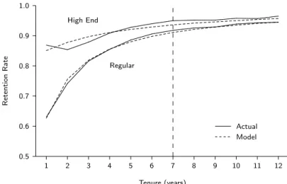
Another plot of interest shows the (aggregate) retention rate as a function of tenure. The model-based retention rate numbers (as computed using (8)) are plotted in Figure 5, along with the corresponding observed retention rates as computed from the empirical survivor functions. For both segments, the sBG model accurately tracks the empirical retention rate curves. On one hand, this might not seem surprising since rt and S(t) are so closely related; on the other hand, however, rt is harder to predict accurately since it is not a cumulative number like S(t) and therefore it is more sensitive to period-to-period variations. Despite the existence of certain unexplained “blips” as in year 2 for the High End segment, the tracking/prediction plot forrt is very impressive through year 12 and there is every reason to believe that the model would continue to perform well over an even longer future horizon.
For both segments we note that the retention rates are an increasing function of the length of a customer’s relationship with the firm. The important point to emphasize, once again, is that the sBG “story” assumes that these apparent dynamics are simply a result of heterogeneity; any given individual has a constant (but unknown) retention probability 1−θ. Unlike the conventional wisdom about customer retention, it isnota story of individual customers becoming increasingly loyal as they develop a deeper relationship with the firm, etc. Thus the observed phenomenon of increasing retention rates is simply a sorting effect in a heterogeneous population (i.e., the high churn customers drop out early in the observation period, with the remaining
1 2 3 4 5 6 7 8 9 10 11 12 Tenure (years) 0.5 0.6 0.7 0.8 0.9 1.0 Retention Rate ... ... ... ... ... ... ... ... ... ... ... ... ... Actual ... ... ... ... ... ... ... ... ... ... ... ... ... ... ... Model High End Regular
Figure 5: Actual versus model-based estimates of retention rates by tenure for the High End and Regular segments.
customers having lower churn probabilities).
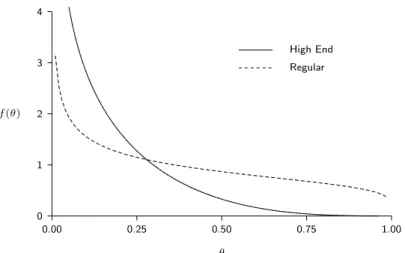
As a final demonstration of the usefulness of the sBG model, we show and contrast the mixing distributions that characterize how the churn probabilities (θ) differ across the individuals in each segment. In Figure 6 we see that both distributions are “reverse J-shaped.” This implies that, within each group, most customers have fairly low churn probabilities, but there is a sizeable sub-segment within each one that will tend to depart very quickly. These patterns suggest that there is a fairly high degree of heterogeneity within each segment, and therefore a model that doesn’t take these cross-customer differences into account will not perform very well, particularly in terms of out-of-sample forecasting. Closer examination shows that the overall “weight” of the distribution for the Regular group is shifted slightly to the right compared to the High End distribution. This reflects the fact that the Regular group has a higher mean churn probability (E(θ) =α/(α+β) = 0.37) compared to that of the High End group (E(θ) = 0.15). It should be clear from Figures 4and 5 that this kind of difference in the means exists, but this plot provides a better idea about the nature of these differences at a more fine-grained level.
4 Discussion
We have presented the shifted-beta-geometric (sBG) distribution as a model for the duration of customer relationships in a discrete-time contractual setting, and demonstrated that it can
0.00 0.25 0.50 0.75 1.00 θ 0 1 2 3 4 f(θ) ...... ...... ...... ...... ...... ...... ...... ...... ...... ...... ...... High End ... ... ... ... ... ... ... ... ...... ...... ...... Regular
Figure 6: Estimated distributions of churn probabilities for the High End and Regular segments
provide accurate forecasts and other useful diagnostics about customer retention. Furthermore, we have argued that it is preferable to use such a model instead of arbitrary functions of time. In closing, we discuss limits to its application, related models in the direct marketing literature, possible extensions to the basic model, and some practical implementation issues.
4.1 Limits to Application
The practical problem that drove the development of this model is a desire to project an empirical survivor function beyond the observed time horizon of our dataset. The ability to perform this projection is central to any attempts to compute CLV or other metrics such as expected tenure if we wish to avoid “truncation” problem associated with computing these quantities using just the observed survival data. For this particular problem, this simple model should be the first tool the researcher pulls out his toolkit.
There are other churn-related problems where this should not be the case. In particular, there is a broad literature on churn modeling in which logit models (and far more sophisticated statistical models and data mining methodologies) are used to determine the correlates of churn (Berry and Linoff 2004; Parr Rud 2001). The resulting models can then be used to identify which customers are at risk of churning in the next period so that retention-oriented marketing resources can be targeted at them. Many of the covariates included in these models will vary from period to period (e.g., number of contacts with the customer service department), and
changes in these variables can be strong predictors of customer defection.
However these models cannot easily be used to address the problem of projecting the survivor function into the future, as we do not have future values of the time-varying covariates. It is therefore important to use the right model for the task at hand, and to acknowledge the limitations to application of any model we develop.
We have referred to the sBG distribution as a model for the duration of customer relation-ships in a discrete-time contractual setting. Many readers will have glanced over the words “discrete-time” and “contractual” without reflecting on their significance. However, they are very important as we seek to understand when and where it is appropriate to use the model presented in this paper.
• By “discrete-time” we mean that transactions can only occur at fixed points in time (such as the annual renewal cycles for most professional organizations). This is in contrast to continuous-time, where the transactions can only occur at any point in time (such as the cancelation of basic utility contracts).
• In a “contractual” setting, the time at which the customer becomes inactive is observed (e.g., when the customer fails to renewal his subscription). This is in contrast to a “non-contractual” setting, where the absence of a contract or subscription means that the point in time at which the customer becomes inactive is not observed by the firm (such as a catalog retailer). The challenge is how to differentiate between a customer who has ended his “relationship” with the firm versus one who is merely in the midst of a long hiatus between transactions.
This leads to a two-dimensional classification of customer bases: opportunities for transactions (continuous vs discrete) and type of relationship with customers (noncontractual vs contractual). The model developed in this paper is for just one of the four possible business contexts.
In continuous-time contractual settings, we should not use the sBG model. Rather, we should use its continuous-time analog, the exponential-gamma (EG) distribution (also known as the Lomax distribution or the “Pareto distribution of the second kind”). Such a model assumes that the duration of an individual customer’s relationship with the firm is characterized by the
exponential distribution, and that heterogeneity in “departure rates” is captured by a gamma distribution (Hardie et al. 1998; Morrison and Schmittlein 1980).
Models for noncontractual settings are more complicated because the time at which a cus-tomer becomes inactive, and the likelihood that it has occurred at all, must be inferred from the transaction history. For continuous-time noncontractual settings we have the Pareto/NBD (Schmittlein et al. 1987) and BG/NBD (Fader et al. 2005) models, while for discrete-time non-contractual settings we have the BG/BB model (Fader et al. 2004).
4.2 Related Probability Models and Extensions
“List falloff” is an important phenomenon in direct marketing. The basic idea is that the response rate from the first mailing to a prospect list is usually higher than that of the second mailing, which in turn is higher than that for the third mailing, and so on. Buchanan and Morrison (1988), hereafter BM, presented a simple probability model of list falloff and showed how the model can be used to determine how many more mailings should be sent to a prospect list, given the observed response rates for the first two mailings. Their model is based on assumptions similar to those behind the sBG model: (i) each person responds to a direct mail solicitation with constant probability p, and (ii) p varies across the population according to a beta distribution. While BM base their framework on the beta-binomial model, it could have been derived as an sBG model (e.g., the mailing on which the prospect responds to the offer is characterized by the shifted geometric distribution). As such, it is possible to identify clear relationships between some of the results in this paper (e.g., rt and S(t)) and some quantities of interest in a list-falloff setting.
The BM framework is extended by Rao and Steckel (1995) to incorporate (time-invariant) descriptor variables such as age, income, and sex. This is accomplished using the beta-logistic model (Heckman and Willis 1977), which extends the beta-binomial model by making the model parameters functions of the descriptor variables. By a similar logic, the effects of time-invariant covariates could be incorporated in the sBG model by makingα andβ functions of the descrip-tor variables. Incorporating the effects of time-varying covariates (e.g., marketing-mix effects, seasonality) is more complicated. The key is to bring in all of these factors at the right level, i.e,
at the level of the latent parameter of interest (in this caseθ) instead of just “jamming” different covariate effects into a regression-like model. (See Schweidel et al. (2006) for an discussion of how to do this in a continuous-time contractual setting.) However, as noted in Section 4.1, we question the value of such a extension given our modeling objective (i.e., projecting the empirical survivor function beyond the observed time horizon of our dataset).
Both the sBG model and its continuous-time analog (the EG model) are based on the assumption that the commonly observed phenomenon of increasing retention rates is due entirely to heterogeneity; individual-customer-level retention rates are assumed to be constant. If we wish to allow for the possibility of time dynamics at the level of the individual customer, we can no longer characterize the duration of an individual’s relationship with the firm using either the shifted-geometric or exponential distribution, both of which have the “memoryless” property (i.e., the probability of survival tos+t, given survival tot, is the same as the initial probability of survival to s). In a continuous-time setting, we can accommodate this effect by assuming that individual lifetimes can be characterized by the Weibull distribution, which allows for an individual’s risk of cancelling his contract to increase or decrease as the length of the relationship with the firm increases. In a discrete-time contractual setting, this leads to the beta-discrete-Weibull (BdW) model (Fader and Hardie 2006), which is a generalization of the sBG model, while in a continuous-time contractual setting, this leads to a generalization of the EG model, the Weibull-gamma (WG) model (Hardie et al. 1998; Morrison and Schmittlein 1980).
4.3 Implementation Issues
Our treatment of how to estimate the sBG model parameters (Appendix B) assumes we are fitting the model to data for just one cohort of customers. But in practice, we will frequently have data for more than one cohort, where cohorts are defined by time of acquisition (and possibly acquisition channel, product class, etc.) When faced with data for multiple cohorts, an important model implementation issue is to choose among three possible approaches: (1) to pool the cohorts and estimate a single set of model parameters across them, (2) to estimate a separate set of model parameters for each cohort, or (3) to use a “beta-logistic” version of the sBG with cohort-specific dummy variables. Our decision of how to move ahead is influenced
by our beliefs as to whether or not we can view each cohort as the realization of a common underlying contract duration process. The two datasets examined above demonstrate that we can expect to see some cross-cohort differences. Schweidel et al. (2006) examine this issue more broadly in a continuous-time setting.
When we have multiple cohorts defined by time of acquisition, the problem with fitting separate models to each cohort is that every new cohort has one less period of information than its temporal predecessor, which may result in less confidence in the model parameter estimates for the cohorts with fewer data points. The natural starting point in such a situation is to pool the cohorts, assuming that each cohort is the realization of a common underlying contract duration process and to estimate one set of parameters using all the data. A more elegant solution would be to add another layer of heterogeneity on to the model. That is, we would assume that α and β themselves are distributed across across cohorts according to some parametric distribution. Using a hierarchical Bayes formulation, this would enable the cohorts with fewer data points could “borrow” information about the possible values of α and β from the earlier cohorts, rather than relying on the cohort-specific data alone.
Appendix A: Steps in Model Derivation
In this appendix we walk through the derivations of the key mathematical results presented in this paper.
We first note three definitions and results that are central to the derivations that follow. • The beta functionB(α, β) is defined by the integral
B(α, β) =
1
0 θ
α−1(1−θ)β−1dθ, α, β >0. (A1)
Note that B(α, β) is simply notation for the definite integral on the right-hand side of (A1).
• The beta function can be expressed in terms of gamma functions:
B(α, β) = Γ(Γ(αα)Γ(+ββ)). (A2) • For the purposes of this paper, the only thing we need to know about the gamma function
is its so-called recursive property:
Γ(x+ 1)
Γ(x) =x . (A3)
Derivation of (5)
We derive the sBG expression for P(T = t) in the following manner. If θ were known, the probability of dropping out in periodtwould simply be the geometric probabilityθ(1−θ)t−1. But sinceθis unobserved (and assumed to be distributed randomly across the population),P(T =t) for a randomly-chosen individual is the expected value of the shifted-geometric probability of dropping out in period t (conditional on Θ =θ), where the expectation is with respect to the beta distribution for Θ, EP(T =t|Θ =θ). (That is, we weight eachP(T =t|Θ =θ) by the probability of that value of θoccurring, f(θ).) Since Θ is a continuous random variable, this is computed as
P(T =t|α, β) = 1 0 P (T =t|Θ =θ) geometric f(θ|α, β) beta dθ = 1 0 θ(1−θ) t−1θα−1(1−θ)β−1 B(α, β) dθ
which, combining terms and moving all non-θ elements to the left of the integral sign,
= 1
B(α, β)
1
0 θ
α(1−θ)β+t−2dθ .
Looking closely at the integral, we see that it is simply the integral expression for the beta function (A1) with parameters α+ 1 and β+t−1. Therefore,
P(T =t) = B(α+ 1B(, βα, β+)t−1).
(The expression for the sBG survivor function (6) is derived in a similar manner.)
Derivation of (7)
In order to derive the forward-recursion formula used to compute sBG probabilities, we first note that
P(T = 1|α, β) = B(Bα(+ 1α, β, β) )
which, expressing the beta functions in term of gamma functions (A2), = Γ(Γ(αα+ 1)Γ(+β+ 1)β)Γ(Γ(αα)Γ(+ββ)) = Γ(Γ(α+ 1)α) Γ(Γ(α+α+β+ 1)β) .
Recalling the recursive nature of the gamma function (A3), Γ(α+ 1)/Γ(α) =α and Γ(α+β+ 1)/Γ(α+β) =α+β. Therefore,
P(T = 1|α, β) = α+αβ .
But how does this help us computeP(T =t) for t= 2,3, . . .? Reflecting on the identity
P(T =t) = P(PT(T==t−t)1)×P(T =t−1),
if we have a simple expression for the ratio P(T = t)/P(T = t−1), we can easily compute
P(T = 2) given the value ofP(T = 1) =α/(α+β). Given the value ofP(T = 2), we can then computeP(T = 3), and so on.
Recalling (5), we have P(T =t) P(T =t−1) = B(α+ 1, β+t−1) B(α, β) B(α+ 1, β+t−2) B(α, β) = BB((αα+ 1+ 1, β, β++tt−−1)2)
which, expressing the beta functions in term of gamma functions (A2) and cancelling terms, = Γ(Γ(ββ++tt−−1)2)Γ(Γ(αα++ββ++t−t)1)
which, recalling the recursive nature of the gamma function (A3), = α+β+β+t−t−2 1.
The complete forward-recursion formula naturally follows.
Derivation of (8)
We derive the expression for the retention rate as implied by the sBG model by substituting the expression for the sBG survivor function (6) into (2) and simplifying:
rt= BB(α, β(α, β+)t)
B(α, β+t−1)
B(α, β) = BB(α, β(α, β++t−t)1)
which, expressing the beta functions in term of gamma functions (A2) and cancelling terms, = Γ(Γ(β+β+t−t)1)Γ(Γ(α+α+β+β+t−t)1)
which, recalling the recursive nature of the gamma function (A3), = α+β+β+t−t−1 1.
Appendix B: Implementing the Model in Excel
In this appendix we show how to compute the maximum likelihood estimates the sBG model parameters for the High End dataset using Microsoft Excel. Before providing step-by-step instructions for constructing the worksheet, we briefly review the notion of maximum likelihood estimation.
Suppose we observe a group of n customers for seven periods. We note that n1 customers drop out in the first period, n2 in the second period, . . . , with n7 customers departing in the seventh period. It follows thatn−7t=1nt customers are still active at the end of the seventh period.
Let us assume that the customer lifetimes can be characterized by the sBG distribution. What is the probability that a randomly-chosen customer has a lifetime of one period? The answer is the sBG probabilityP(T = 1|α, β). What is the probability that a randomly-chosen customer has a lifetime of two periods? Answer: the sBG probabilityP(T = 2|α, β). What is the probability that one randomly-chosen customer has a lifetime of one period while another has a lifetime of two periods? Assuming the propensity of one customer to drop out is independent of the behavior of the other customer, it is simply the product of the respective sBG probabilities:
P(T = 1|α, β)P(T = 2|α, β). It follows that, given specific values of the model parameters
α and β, the joint probability of n1 customers departing in the first period, n2 in the second period, . . . ,n7 in the seventh period, andn−7t=1ntcustomers still being active at the end of the seventh period is
P(data|α, β) =P(T = 1|α, β)n1P(T = 2|α, β)n2P(T = 3|α, β)n3
×P(T = 4|α, β)n4P(T = 5|α, β)n5P(T = 6|α, β)n6
×P(T = 7|α, β)n7S(7|α, β)n−7t=1nt. (B1)
However, we do not know the values of α and β, even though we believe that the data come from the sBG distribution.
maximize the probability (or, more formally, thelikelihood) of the observed data. We define the likelihood function as
L(α, β|data) =P(T = 1|α, β)n1P(T = 2|α, β)n2P(T = 3|α, β)n3
×P(T = 4|α, β)n4P(T = 5|α, β)n5P(T = 6|α, β)n6
×P(T = 7|α, β)n7S(7|α, β)n−7t=1nt. (B2)
and use numerical optimization methods (e.g., the Solver add-in in Excel) to find the values of
α and β that maximize this function; these are called themaximum likelihood estimates of the model parameters.4 As the number computed using (B2) will be very small, we usually work with the natural logarithm of the likelihood function, the so-called log-likelihood function:
LL(α, β|data) =7 t=1 ntlnP(T =t|α, β)+ n−7 t=1 nt lnS(7|α, β). (B3) The observant reader will note that we do not actually known, n1, n2, . . . , n7for the two datasets given in Table 1; the data are expressed as percentages of the initial number of customers. Looking closely at (B3), we see that this is not a problem; we can simply factor outn(e.g., n1 becomesn1/n, the proportion of customers who become inactive in the first period). While this will affect the “height” of the maximum point of the log-likelihood function, the location of the maximum (i.e., the values ofα and β) will be unaffected.
So our task is to “code up” this expression for the model log-likelihood function in an Excel worksheet and find maximum likelihood estimates ofαandβby using Solver to find the values of
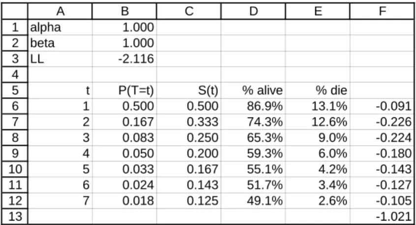
αandβ that maximize the value of this function. The relevant worksheet is shown in Figure B1 and is constructed in the following manner.
• In order to enter expressions forP(T =t|α, β) without an error message appearing (e.g.,
#NUM!or#DIV/0!), we need some “starting values” forα and β. The exact values do not matter — provided they are within the defined bounds — so we start with 1.0 forα and β, locating these parameter values in cells B1:B2, respectively.
4We note that (B1) and (B2) look almost identical, but there is a subtle difference: in (B1), the probability
1 2 3 4 5 6 7 8 9 10 11 12 13 A B C D E F alpha 1.000 beta 1.000 LL -2.116 t P(T=t) S(t) % alive % die 1 0.500 0.500 86.9% 13.1% -0.091 2 0.167 0.333 74.3% 12.6% -0.226 3 0.083 0.250 65.3% 9.0% -0.224 4 0.050 0.200 59.3% 6.0% -0.180 5 0.033 0.167 55.1% 4.2% -0.143 6 0.024 0.143 51.7% 3.4% -0.127 7 0.018 0.125 49.1% 2.6% -0.105 -1.021 Figure B1: Screenshot of Excel Worksheet for Parameter Estimation • We enter the values oft= 1,2, . . . ,7 in cellsA6:A12.
• The corresponding values ofP(T =t|α, β) are computed in cellsB6:B12using the forward-recursion given in (7):
– We computeP(T = 1) by entering=B1/(B1+B2)in cellB6.
– We computeP(T = 2) by entering=($B$2+A7-2)/($B$1+$B$2+A7-1)*B6)in cellB7.
– We copyB7 toB8:B12.
• We compute the values ofS(t|α, β) for t= 1,2, . . . ,7 in cellsC6:C12:
– S(1) is simply 1−P(T = 1), so we enter=1-B6in cell C6.
– Fort >1,S(t) =S(t−1)−P(T =t), so we enter =C6-B7in cellC7.
– We copyC7 toC8:C12.
• The next step is to enter the actual survival data. The proportion for year 1 (0.869) is entered in cell D6, the proportion for year 2 (0.743) is entered in cellD7, and so on down to 0.491 in cell D12 for year 7. (In the worksheet shown in Figure B1, cells D6:D12 are formatted using the percentage style.)
• The proportion of customers dropping out each year, as required for the log-likelihood function, is computed in cellsE6:E12:
– As the proportion of customers who dropped out in year 1 is simply one minus the proportion of customers who are still active at the end of the first year, we enter
=1-D6in cellE6.
– For t >1, the proportion of customers who dropped out in year t is the proportion of customers who are still active at the end of year t−1 minus the proportion of customers who are still active at the end of the yeart. We therefore enter =D6-D7in cellE7and copy it to E8:E12.
• The first seven elements of the log-likelihood function are computed in cells F6:F12: we enter=E6*LN(B6) in cellF6and copy it to E7:E12.
• The final element of the log-likelihood function, that associated with those customers who have survived at least seven years, is entered as=D12*LN(C12) in cellF13.
• The sum of cellsF6:F13is entered in cellB3; this is the value of the log-likelihood function given the values for the two model parameters in cellsB1:B2. (With starting values of 1.0 for both parameters,LL=−2.116.)
We find the maximum likelihood estimates of the two model parameters by maximizing the log-likelihood function. We do this using the Excel add-in Solver, available under the “Tools” menu. The target cell is the value of the log-likelihood, cell B3. We wish to maximize this by changing cells B1:B2. Theconstraints we place on the parameters are thatα andβ are greater than 0. As Solver only offers us a “greater than or equal to” constraint, we add the constraint that cellsB1:B2are ≥a small positive number (e.g., 0.0001) — see Figure B2.
Clicking the Solve button, Solver converges to a solution where the maximum value of the log-likelihood function is −1.611, associated with α = 0.668 and β = 3.806. These are the maximum likelihood estimates of the model parameters. (So as to be sure that we have actually reached the maximum of the log-likelihood function, it is good practice to redo the optimization process using a completely different set of starting values. For example, using starting values of 0.01 and 0.01 (for which LL = −2.742), use Solver to find the maximum of the log-likelihood function. Are the corresponding values of the two model parameters equal to those given above? They should be!)
References
Berry, Michael J. A. and Gordon S. Linoff (2004), Data Mining Techniques: For Marketing, Sales, and Customer Relationship Management, 2nd edition, Indianapolis, IN: Wiley Publishing, Inc.
Buchanan, Bruce and Donald G. Morrison (1988), “A Stochastic Model of List Falloff with Implications for Repeat Mailings,”Journal of Direct Marketing,2(Summer), 7–15.
Fader, Peter S. and Bruce G. S. Hardie (2006), “Customer Base Valuation in a Contractual Setting: The Perils of Ignoring Heterogeneity,” unpublished working paper.
Fader, Peter S., Bruce G.S. Hardie, and Paul D. Berger (2004), “Customer-Base Analysis with Discrete-Time Transaction Data.” [http://brucehardie.com/papers/020/]
Fader, Peter S., Bruce G. S. Hardie, and Ka Lok Lee (2005), “"Counting Your Customers"
the Easy Way: An Alternative to the Pareto/NBD Model,” Marketing Science, 24 (Spring), 275–284.
Kaplan, Edward H. (1982), “Statistical models and mental health: An analysis of records from a mental health center,” M.S. Thesis, Department of Mathematics, Massachusetts Institute of Technology.
Hardie, Bruce G. S., Peter S. Fader, and Michael Wisniewski (1998), “An Empirical Comparison of New Product Trial Forecasting Models,”Journal of Forecasting,17(June–July), 209–229. Heckman, James J. and Robert J. Willis (1977), “A Beta-logistic Model for the Analysis of Sequential Labor Force Participation by Married Women,” Journal of Political Economy, 85
(February), 27–58.
Morrison, Donald G. and David C. Schmittlein (1980), “Jobs, Strikes, and Wars: Probability Models for Duration,”Organizational Behavior and Human Performance,25(April), 224–251. Parr Rud, Olivia (2001),Data Mining Cookbook, New York, NY: John Wiley & Sons, Inc. Rao, Vithala R. and Joel H. Steckel (1995), “Selecting, Evaluating, and Updating Prospects in Direct Marketing,”Journal of Direct Marketing, 9 (Spring), 20–31.
Schmittlein, David C., Donald G. Morrison, and Richard Colombo (1987), “Counting Your Customers: Who They Are and What Will They Do Next?” Management Science,33(January), 1–24.
Schweidel, David A., Peter S. Fader, Peter and Eric T. Bradlow (2006), “Modeling Retention in and Across Cohorts,”http://ssrn.com/abstract=742884.
Vaupel, James W. and Anatoli I. Yashin (1985), “Heterogeneity’s Ruses: Some Surprising Effects of Selection on Population Dynamics,”The American Statistician,39(August), 176–185. Weinberg, Clarice Ring and Beth C. Gladen (1986), “The Beta-Geometric Distribution Applied to Comparative Fecundability Studies,”Biometrics,42(September), 547–560.