Branch and Peg Algorithms for the Simple Plant
Location Problem
Boris Goldengorin Diptesh Ghosh∗ Gerard Sierksma
Faculty of Economic Sciences, University of Groningen, The Netherlands.
SOM-theme A Primary Processes within Firms
Abstract
The simple plant location problem is a well-studied problem in combinatorial optimization. It is one of deciding where to locate a set of plants so that a set of clients can be supplied by them at the minimum cost. This problem of-ten appears as a subproblem in other combinatorial problems. Several branch and bound techniques have been developed to solve these problems. In this paper we present a few techniques that enhance the performance of branch and bound algorithms. The new algorithms thus obtained are called branch and peg algorithms, where pegging refers to assigning values to variables out-side the branching process. We present exhaustive computational experiments which show that the new algorithms generate less than 60% of the number of subproblems generated by branch and bound algorithms, and in certain cases require less than 10% of the execution times required by branch and bound algorithms.
Keywords: Simple Plant Location Problem, Pseudo-Boolean representation, Beresnev function, Branch and Bound, Preprocessing, Pegging.
∗ Corresponding Author: Faculty of Economic Sciences, University of Groningen, P.O. Box 800,
1. Introduction
Given setsI = {1,2, . . . , m}of sites in which plants can be located,J = {1,2, . . . , n} of clients, a vectorF =(fi)of fixed costs for setting up plants at sitesi ∈I, a matrix
C = [cij] of transportation costs from i ∈ I toj ∈ J, and an unit demand at each
client site, the Simple Plant Location Problem (SPLP) is the problem of finding a setS,
∅ ⊂S ⊆I, at which plants can be located so that the total cost of satisfying all client demands is minimal. The costs involved in meeting the client demands include the fixed costs of setting up plants, and the transportation cost of supplying clients from the plants that are set up. A detailed introduction to this problem appears in Cornuejolset al. [12]. The SPLP forms the underlying model in several combinatorial problems, like set covering, set partitioning, information retrieval, simplification of logical Boolean expressions, airline crew scheduling, vehicle despatching (Christofides [6]), assortment (Beresnev et al. [5], Goldengorin [17], Jones et al. [23], Pentico [29, 30], Tripathy et al. [33]), and is a subproblem for various location analysis problems (Revelle and Laporte [31]).
The SPLP is NP-hard (Cornuejolset al. [12]), and many exact and heuristic algorithms to solve the problem have been discussed in the literature. Most of the exact algorithms are based on a mathematical programming formulation of the SPLP. Direct approaches (Schrage [32], Morris [27]) use a branch and bound approach and the strong linear pro-gramming relaxation (SLPR) for computing bounds. However such approaches cannot always output an optimal solution to average-sized SPLP instances in reasonable time. More efficient solution approaches to the SPLP are based on Langrangian duality (Held et al. [22], Beresnev et al. [5]). Computational experience of solving the Lagrangian dual using subgradient optimization have been reported in Cornuejolset al. [10] and Cornuejols and Thizy [11], and using Dantzig-Wolfe decomposition in Garfinkel et al. [15]. Computer codes for solving medium sized SPLP using mixed-integer program-ming systems are also available (Martin and Schrage [26], Van Roy and Wolsey [35]). Polyhedral results for the SPLP polytope have been reported in Trubin [34], Balas and Padberg [1], Mukendi [28], Cornuejolset al. [9], Krarup and Pruzan [24], Cho et al. [7], and Choet al. [8]. In theory, these results allow us to solve the SPLP by applying the simplex algorithm to SLPR, with the additional stipulation that a pivot to a new ex-treme point is allowed only when this new exex-treme point is integral. Although some computational experience using this method has been reported in the literature (Guig-nard and Spielberg [20]), efficient implementations of this pivot rule are not available. Results of computational experiments with Lagrangian heuristics for medium sized in-stances of the SPLP have been reported in Beasley [2]. Large-sized SPLP inin-stances
can be solved using algorithms based on refinements to a dual-ascent heuristic proce-dure to solve the dual of LP-relaxation of the SPLP (K¨orkel [25]), combined with the use of the complementary slackness conditions to construct primal solutions (Erlenkot-ter [14]). Preprocessing rules, which form a common component in branch and bound implementations, are strangely never explicitly discussed in the available literature on computational experiences with the SPLP.
The pseudo-Boolean representation of the SPLP facilitates the construction of rules to reduce the size of SPLP instances (Beresnevet al. [5], Cornuejols et al. [12], Dearing et al. [13], Goldengorin et al. [19], Veselovsky [36], etc.). These rules have never been used in the explicit description of any algorithm for the SPLP in the available litera-ture. In this paper we propose branch and bound based algorithms called branch and peg algorithms, which use these rules, not only for preprocessing, but also as a tool either to solve a subproblem or to reduce its size. They also use information from a pseudo-Boolean representation of the SPLP to compute efficient branching functions. For the sake of simplicity, we use a common depth first branch and bound scheme in our implementations and a simple combinatorial bound, but the concepts developed herein can easily be implemented in any of the algorithms cited above. Our implemen-tations satisfy our purpose in this paper, which is to test the superiority of branch and peg algorithms over branch and bound algorithms using the same bound.
The remainder of this paper is organized as follows. In Section 2 we describe a pseudo-Boolean representation of the SPLP. In Section 3 we describe branch and peg algo-rithms in detail, and our computational experience with them on randomly generated instances as well as some benchmark instances from Beasley [2] as benchmark in-stances for our computational experiments. We summarize the paper in Section 4 and propose directions for further research.
2. A Pseudo-Boolean Approach to SPLP
The pseudo-Boolean approach to solving the SPLP (Hammer [21], Beresnev [4]) is a penalty-based approach that relies on the fact that any instance of the SPLP has an optimal solution in which each client is supplied by exactly one plant. This implies, that in an optimal solution, each client will be served fully by the plant closest to it. Therefore, it is sufficient to determine the sites where plants are to be located, and then use a minimum weight matching algorithm to assign clients to plants.
An instance of the SPLP can be described by am-vectorF =(fi), and am×nmatrix
C= [cij];m, n≥1. We assume that elements ofF andCare nonnegative. We will use
them×(n+1)augmented matrix [F|C]as a shorthand for describing an instance of the SPLP. The total costf[F|C](S)associated with a solutionSconsists of two components,
namely the fixed costsi∈Sfi and the transportation costs
j∈Jmin{ci,j|i ∈S}; i.e.
f[F|C](S)= i∈S fi + j∈J min{ci,j|i ∈S},
and the SPLP is the problem of finding
S∈arg min{f[F|C](S): ∅ ⊂S⊆I}. (1)
In the remainder of this section we describe the pseudo-Boolean formulation of the SPLP due to Beresnev [4].
A m× n ordering matrix = [πij] is a matrix each of whose columns j =
(π1j, . . . , πmj)T define a permutation of 1, . . . , m. Given a transportation matrixC, the
set of all ordering matricessuch thatcπ1jj ≤cπ2jj ≤ · · · ≤cπmjj, forj =1, . . . , n,
is denoted byperm(C). Defining
yi =
0 ifi∈S
1 otherwise, for eachi=1, . . . , m (2)
we can indicate any solutionSby a vector y =(y1, y2, . . . , ym). The fixed cost
com-ponent of the total cost can be written as
FF(y)= m
i=1
fi(1−yi). (3)
Given a transportation cost matrixC, and an ordering matrix ∈ perm(C), we can denote differences between the transportation costs for eachj ∈J as
c[0, j] = cπ1jj, and
c[l, j] = cπ(l+1)jj −cπljj, l=1, . . . , m−1.
Then, for eachj ∈J,
min{ci,j|i ∈S} = c[0, j] +c[1, j] ·yπ1j +c[2, j] ·yπ1j ·yπ2j + · · · +c[m−1, j] ·yπ1j· · ·yπ(m−1)j = c[0, j] + m−1 k=1 c[k, j] · k r=1 yπrj,
so that the transportation cost component of the cost of a solution y corresponding to an ordering matrix∈perm(C)is
TC,(y)= n j=1 c[0, j] + m−1 k=1 c[k, j] · k r=1 yπrj . (4)
Combining (3) and (4), the total cost of a solution y to the instance[F|C]corresponding to an ordering matrix∈perm(C)is given by the pseudo-Boolean polynomial
f[F|C],(y) = FF(y)+TC,(y) = m i=1 fi(1−yi)+ n j=1 c[0, j] + m−1 k=1 c[k, j] · k r=1 yπrj .(5)
It can be shown (Goldengorinet al. [19]) that the total cost functionf[F|C],(·)is
iden-tical for all ∈ perm(C). We call this pseudo-Boolean polynomial the Beresnev function B[F|C](y) corresponding to the SPLP instance[F|C]and ∈ perm(C). In
other words
B[F|C](y)=f[F|C],(y)where∈perm(C). (6)
We can formulate (1) in terms of Beresnev functions as
y ∈arg min{B[F|C](y):y∈ {0,1}m,y=1}. (7)
Beresnev functions assume a key role in the development of the algorithms described in the next section.
3. Branch and Peg Algorithms
In this section we describe enhancements to branch and bound (BnB) algorithms to solve SPLP instances. The enhanced algorithms use a rule based on Beresnev functions to peg variables in subproblems, i.e. to determine before branching, whether plants will (or will not) be located at certain sites in the current subproblem. This rule, used on the initial instance, forms a preprocessing rule. The other enhancement that we propose, is the use of Beresnev functions to devise effective branching functions. The new algorithms are collectively calledbranch and peg (BnP) algorithms. We use a depth first search strategy in our algorithms, but the concepts can be used unchanged in best first search.
The following terms are used in the remainder of this section. A solution to a SPLP instance with|I| = mand|J| = nis a vector y of lengthm, defined on the alphabet
{0,1,#}.yj =0 (respectively,yj =1) indicates that a plant is located (respectively, not
located) at the site with indexj.yj = # indicates that no decision regarding locating
a plant at the site with index j has been incorporated in the solution. A solution y withyj =# for somej is called apartial solution, while all other solutions are called
complete solutions. The process of setting the value ofyj for any indexjin any partial
solution y to 0 or 1 is calledpegging the variable. Ifyj =#, thenyj is called anopen
variable, and ifyj =0 or 1, it is called apegged variable.
The pseudo-Boolean representation of the SPLP allows us to develop rules using which we can peg certain variables in a solution by examining the coefficients of the Beres-nev functions. The rule that we use here is described in Goldengorinet al. [19] as a preprocessing rule. We assume, without loss of generality, that the instance is not sep-arable, i.e. we cannot partitionIinto setsI1andI2, andJ into setsJ1andJ2, such that
the transportation costs from sites inI1to clients inJ2, and from sites inI2to clients
in J1 are not finite. We also assume without loss of generality, that the site indices
are arranged in non-increasing order offi +
j∈Jcij values. We include the proof of
correctness of this rule for the sake of completeness.
Pegging Rule (Goldengorinet al. [19]) LetB[F|C](y)be the Beresnev function
corre-sponding to the SPLP instance[F|C] in which like terms have been aggregated. Let ak = (
j:π1j=kc[1, j])−fk be the coefficient of the linear term corresponding to
yk and let tk =
n
j=1
j:k∈{π1j,...,πpj} m−1
p=2c[p, j] be the sum of the coefficients of all
non-linear terms containingykfor each site indexk. Then the following hold.
(a) Ifak ≥0, then there is an optimal solution yin whichyk =0, else
(b) ifak+tk ≤ 0, then there is an optimal solution y in whichyk =1, provided
yi =1for somei =k. PROOF.
(a) Supposeak ≥0. Let us consider a solution y in whichyk =1 and a solution yin
whichyi =yi for eachi=k, andyk =0. NowB[F|C](y)−B[F|C](y)≥ak ≥0.
(b) Next suppose thatak+tk ≤0. Consider two solutions y and y, such thatyi =yi
for eachi=k,yk =0, andyk =1. Then
B[F|C](y)−B[F|C](y) = { m i=1 fi(1−yi)+ n j=1 m−1 p=1 [p, j] p r=1 yπrj} − { m i=1 fi(1−yi)+ n j=1 m−1 p=1 [p, j] p r=1 yπrj} = {−fkyk − m i=1 i=k fiyi A + n j=1 j:k∈{π1j,...,πpj} m−1 p=1 [p, j] p r=1 yπrj + n j=1 j:k∈{π1j,...,πpj} m−1 p=1 [p, j] p r=1 yπrj} B − {−fkyk− m i=1 i=k fiyi C + n j=1 j:k∈{π1j,...,πpj} m−1 p=1 [p, j] p r=1 yπ rj + n j=1 j:k∈{π1j,...,πpj} m−1 p=1 [p, j] p r=1 yπrj D } (8)
Notice that the terms marked AandC cancel each other since yi = yi when
i = k, as do the terms marked B andD. Cancelling these terms and setting yk =0 andyk =1 in (8) we obtain B[F|C](y)−B[F|C](y) = {−fk+ n j=1 j:k∈{π1j,...,πpj} m−1 p=1 c[p, j] p r=1 yπrj} (9)
which, on separating the linear and non-linear terms = {ak+ n j=1 j:k∈{π1j,...,πpj} m−1 p=2 c[p, j] p r=1 yπ rj}. (10)
An upper bound to (10) isak+tk, which is obtained by settingyi=1 for each
i ∈ I, since all non-linear terms in the Beresnev function have non-negative coefficients. Thus
B[F|C](y)−B[F|C](y)≤(ak+tk)≤0. (11)
Hence y is preferable to y. This shows thatyk = 1 in an optimal solution. Of
course, ify
i = 1 for alli = k, then settingy
k to 1 would yield an infeasible
solution.
Note thattk ≥ 0 for each index k, since the non-linear terms of the Beresnev function
are non-negative. Thusak+tk ≤0 ⇒ ak ≤0. Iftk =0, then there is a possibility of
akbeing equal to zero, but this possibility is taken care of in the first part of the rule.
The importance of the ordering of the site indices is demonstrated in the following lemma.
Lemma 3.1 Ifak < 0 andak +tk ≤ 0 for eachk ∈ I inB[F|C](y)for the SPLP instance[F|C], then an optimal solution would be(1,1, . . . ,1,0)assuming that the
site indices are arranged in non-increasing order offi+
j∈Jcij values.
PROOF. Let us initially relax the constraint y =1 in (7). In such a case it is easy to
see that the optimal solution would be y=1 (from (11)). If we reimpose the constraint,
we need to set one or moreyk values to 0. Changing yk = 0 for any variable k ∈ I
increases the value of the Beresnev function byfk+
j∈Jckj. Note that settingyk =0
does not affect the non-positive nature of ai +ti, i = k, since this operation does
not affectai and can only reduce the value ofti. Also note that setting any additional
variableyi,i =kto 0 cannot reduce the value of Beresnev function sinceai <0 and
The lemma above is illustrated by the following example. Consider a SPLP instance [F|C],m=n=3, in whichF =(99,100,98)and C= 100 100 1316 13 16 0
The Beresnev function for this instance is
B[F|C]=297−89y1−90y2−85y3+9y1y2+3y1y3.
It is clear thatak < 0 and ak +tk < 0 for k = 1, 2, and 3. Therefore the Pegging
Rule will solve this instance completely, setyk =1 the first two sites it encounters, and
setyk =0 for the last site. However, the solution would be correct only if the last site
encountered has the lowestfi +
j∈Jcij value, i.e., if site 1 is considered after sites
2 and 3. In general therefore, the sitesi should be ordered in non increasing values of fi+
j∈Jcij.
In the remainder of this section, we will assume the existence of a procedure P eg -P artialSolution, which implements the Pegging Rule. It accepts a partial solution as input, repeatedly applies the Pegging Rule above until no further pegging is possible, and returns the solution thus obtained. (Note that the solution returned by this procedure will, in general, be a partial solution.)P egP artialSolution will be used for prepro-cessing in both BnB and BnP algorithms, as well as for pegging variables in partial solutions in the BnP search tree. We will call the solution obtained after preprocessing, (implemented by runningP egP artialSolutionon the partial solution(##· · ·#),) the initial solution. This solution forms the root of the BnP and BnB search trees.
The choice of the variable to branch on is critical for the success of a branch and bound scheme. The following trivial branching function can be used in the absence of any prior knowledge regarding the suitability of the variable to branch on.
Branching Function 1 Return the open variable with the minimum index in the cur-rent subproblem.
However, we could use information from the coefficients of the Beresnev function to create more effective branching functions.
Consider a subproblemP in which the partial solution, after being pegged by theP eg -P artialSolution procedure, is y. For each variable yk in y that is still open, let yk0
be obtained by forcibly pegging yk to 0, and running P egP artialSolution on the
resultant solution; let φk0 be the number of open variables in yk0. Similarly, let yk1
be obtained by forcibly pegging yk to 1 in y, and running P egP artialSolution on
the resultant solution; letφk1 be the number of open variables in yk1. If we want to
obtain a quick upper bound for the objective value of the optimal solution to P by solving its subproblems by pegging, thenφk =min(φk0, φk1)is a good measure of the
suitability ofyk as a branching variable. (Other combinations ofφk0andφk1, such as
φk0+φk1
2 could also be used, but our preliminary experimentation shows that these do not
cause significant differences in the results obtained.) A branching function based on such a measure, can be expected to generate relatively few subproblems while solving a SPLP instance. However, the calculations involved would, in general, take excessive time. As a compromise therefore, we could use a branching function that generates the ordering of the indices once for the initial solution and uses it for all subproblems. This branching function is described below.
Branching Function 2 For each open variable yk in the initial solution y, let φk0
(respectively,φk1) be the number of open variables in the solution obtained by setting
yk =0 (respectively,yk =1) in the initial solution and runningP egP artialSolution on it. Define the fitnessφj of the variableyj as
φj =
min(φj0, φj1) ifyj is open in the initial solution,
∞ otherwise.
Return the open variableyj for whichφj is minimal.
A third branching function may be devised in the following manner. Consider a sub-problemP in which the partial solution, after being pegged byP egP artialSolution, is y. Recall that the Pegging Rule pegs any variableyk withak ≥ 0 to 0, and any
vari-ableyk withtk+ak ≤0 to 1. Therefore, for each variableyk that has not been pegged
we conclude thatak < 0 andtk +ak > 0. yk would have been pegged to 0 in this
solution if the coefficient of linear term involvingyk in the Beresnev function would
have been increased by−ak. It would have been pegged to 1, if the same coefficient
would have been decreased bytk+ak. Therefore we could useφk =max(−ak, tk+ak)
as a measure of the improbability ofyk being pegged in any subproblem ofP. If we
want to reduce the size of the branch and bound tree by pegging such variables, then we can consider a branching function that returns the open variableyj having the largest
function that generates the ordering of indices once for the initial solution and uses it for all subproblems.
Branching Function 3 Define the fitnessφj of the variableyj as
φj =
max{−aj, tj+aj} ifyj is open in the initial solution,
−∞ otherwise.
Return the open variableyj for whichφj is maximal.
In the remainder of this section we will assume the existence of a procedureF indBran -chingV ariablethat takes a partial solution as input, and returns the best variable to branch on.
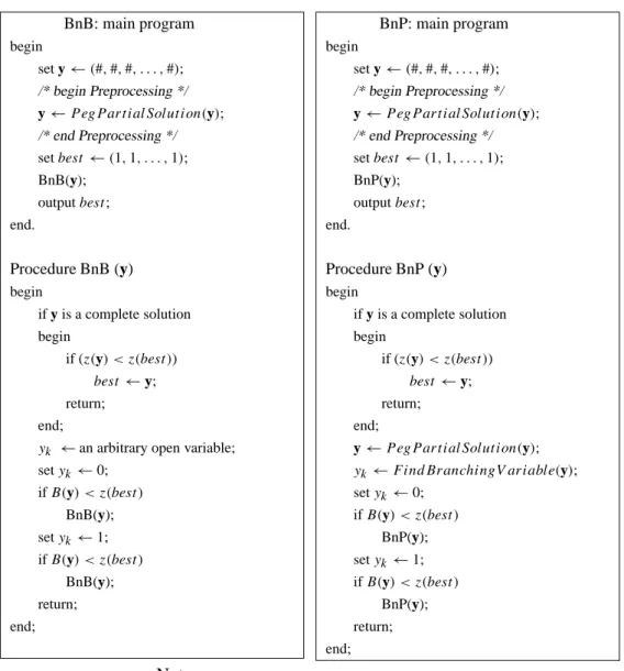
The pseudocodes for recursive implementations of BnB and BnP algorithms are pre-sented in Figure 3.1. We implemented these algorithms to evaluate their performance on randomly generated problem instances as well as on benchmark problem instances. The BnB algorithm was implemented using Branching Function 1. The BnP algorithms were implemented using each of the three branching functions. Notice that we use preprocessing (using theP egP artialSolutionfunction) for both BnB and BnP algo-rithms. The pseudocode for the bound used in all the implementations is presented in Figure 3.2. It is an adaptation of a similar bound for general supermodular functions (refer Goldengorin et al. [18]) for the SPLP. The algorithms were implemented to al-low a maximum execution time of 600 CPU seconds per SPLP instance. The codes were written in C, and run on a Pentium 200 MHz computer running Redhat Linux. The random problem instances were generated in sets of 10 instances each. A prob-lem set is identified by three parameters — the cardinality of the setI (i.e.m), that of the setJ (i.e. n), and the density indexγ. γ indicates the probability with which an element in the cost matrix has a finite value. Care is taken that, while generating the instances, value each client can be supplied from a plant in at least one of the candidate sites at finite cost regardless of theγ. In each of the randomly generated instances, the fixed costs were chosen from a uniform distribution supported on[10.0,1000.0], and the finite transportation costs were chosen from a uniform distribution supported on
[1.0,100.0]. The benchmark instances were obtained from the OR-Library [3]. There are twelve SPLP problem instances in this library, four with m = 16 and n = 50, four withm = 25 andn = 50, and four withm = n =50. The density index of the transportation cost matrices for all these instances wasγ =1.0.
BnB: main program
begin
set y←(#,#,#, . . . ,#); /* begin Preprocessing */ y←P egP art ialSolut ion(y); /* end Preprocessing */ setbest←(1,1, . . . ,1); BnB(y); outputbest; end. Procedure BnB (y) begin if y is a complete solution begin if (z(y) < z(best )) best←y; return; end;
yk ←an arbitrary open variable;
setyk ←0; ifB(y) < z(best ) BnB(y); setyk ←1; ifB(y) < z(best ) BnB(y); return; end; BnP: main program begin set y←(#,#,#, . . . ,#); /* begin Preprocessing */ y←P egP art ialSolut ion(y); /* end Preprocessing */ setbest←(1,1, . . . ,1); BnP(y); outputbest; end. Procedure BnP (y) begin if y is a complete solution begin if (z(y) < z(best )) best←y; return; end;
y←P egP art ialSolut ion(y);
yk←F indBranchingV ariable(y); setyk ←0; ifB(y) < z(best ) BnP(y); setyk ←1; ifB(y) < z(best ) BnP(y); return; end; Note:
best: the best solution found so far;
z(·): a function to compute the cost of a solution.
B(·): a function to compute the bound from a partial solution.
Procedure B (y: Partial Solution) begin S= {j :yj =0}; T = {j :yj =1}; l1=z(S)−k∈T\Smax{0, z(S)−z(S+k)}; l2=z(T )− k∈T\Smax{0, z(T )−z(T −k)}; return max{l1, l2}; end;
Note:z(P )is assumed to compute the cost of a solution y such thatyk =0 ⇐⇒ k∈P.
Figure 3.2: Pseudocode for the bound used in the implementations
Tables 3.1 to 3.4 present the results of our computations. Table 3.1 shows the number of problem instances in each data set that were solved by the various algorithms within the stipulated time. Tables 3.2 and 3.3 make a comparative study of the average number of subproblems generated by each of the algorithms and the average execution times, based on the instances in the set that were solved by all the algorithms within the stip-ulated time. Table 3.4 summarizes our computational experience with the benchmark instances in the OR-Library, presenting both the number of subproblems generated and the execution times required by the algorithms.
Table 3.1: Number of instances in each set solved within 600 CPU seconds
BnB BnP m n γ Branching Function 1 2 3 30 50 0.25 10 10 10 10 0.50 10 10 10 10 0.75 10 10 10 10 1.00 10 10 10 10 40 50 0.25 6 6 6 10 0.50 10 10 10 10 0.75 10 10 10 10 1.00 10 10 10 10 50 50 0.25 1 2 2 8 0.50 4 7 7 10 0.75 10 10 10 10 1.00 10 10 10 10
Table 3.2: The average number of subproblems generated by the algorithms
Number of BnB BnP m n γ common Branching Function
instances 1 2 3 30 50 0.25 10 24330.4 13700.4 13463.4 5573.0 0.50 10 12769.6 6859.0 6859.0 4448.4 0.75 10 5426.7 2014.8 1969.6 2635.9 1.00 10 3301.5 326.7 211.1 203.5 40 50 0.25 6 104624.8 59593.7 53771.3 12887.5 0.50 10 51927.5 26103.9 26103.9 12218.2 0.75 10 15420.8 5829.7 5829.7 6400.5 1.00 10 8799.5 806.6 481.8 498.3 50 50 0.25 * 0.50 4 62991.25 29188.25 29188.25 17732.25 0.75 10 37898.2 14327.6 14327.6 13043.5 1.00 10 19266.2 1391.9 766.5 932.0 * There was only one instance in common.
Table 3.3: The average execution times required by the algorithms
Number of BnB BnP m n γ common Branching Function
instances 1 2 3 30 50 0.25 10 34.190 27.485 26.843 11.074 0.50 10 20.515 15.252 15.145 9.252 0.75 10 8.194 4.966 4.843 5.371 1.00 10 4.355 0.916 0.698 0.742 40 50 0.25 6 240.357 186.698 164.843 41.708 0.50 10 131.790 58.297 90.792 40.553 0.75 10 38.862 22.656 22.407 21.126 1.00 10 19.482 3.184 2.189 2.535 50 50 0.25 * 0.50 4 225.255 152.065 150.498 92.313 0.75 10 139.090 76.566 75.898 62.987 1.00 10 62.634 7.626 4.781 6.417 * There was only one instance in common.
Table 3.4: Computational experience with the instances in the OR-Library
Number of Subproblems Execution Times Instance m n BnB BnP BnB BnP
Branching Function Branching Function
1 2 3 1 2 3 cap71 30 50 24 18 19 14 <0.01 <0.01 0.01 0.01 cap72 30 50 37 18 21 13 <0.01 <0.01 0.01 0.01 cap73 30 50 194 130 63 65 0.08 0.07 0.03 0.03 cap74 30 50 63 55 11 37 0.01 0.01 0.01 0.01 cap101 40 50 151 92 92 100 0.05 0.04 0.06 0.07 cap102 40 50 567 325 138 965 0.37 0.31 0.12 0.79 cap103 40 50 2054 589 71 198 1.54 0.62 0.09 0.24 cap104 40 50 943 268 38 72 0.74 0.27 0.09 0.08 cap131 50 50 92543 14148 2167 8016 189.88 35.99 6.24 29.61 cap132 50 50 58564 11234 1226 6992 96.82 22.93 3.29 17.94 cap133 50 50 57697 6459 503 1937 116.88 16.92 1.58 5.92 cap134 50 50 4134 744 125 307 7.57 1.84 0.43 1.05
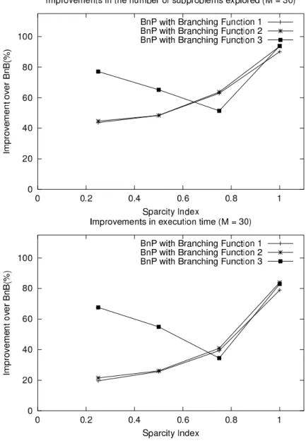
The tables show that BnP algorithms in general perform much better than BnB algo-rithms using the same combinatorial bound. They generate less than 60% of the num-ber of subproblems, and require less than 80% of the execution time for instances with sparse transportation cost matrices. For dense transportation cost matrices, the perfor-mance of BnP algorithms is much better. They generate less than 10% of the number of subproblems, and require less than 10% of the execution time. The relative perfor-mance of these algorithms improve slightly as the size of the instances increase. The BnB algorithm and BnP algorithms using Branching Functions 1 and 2 find instances with low values ofγ more difficult to solve. However BnP algorithms using Branching Function 3 solve these instances efficiently. Figure 3.3 presents the improvements by the BnP algorithms over BnB algorithms, both in terms of the number of subproblems generated and in terms of the execution times. The shapes of the component graphs do not change for problem instances of larger size. Based on these observations we can conclude that it is better to run a BnP algorithm that uses Branching Function 2 if the transportation matrix is dense (i.e.γ 0.6), and to run a BnP algorithm that uses Branching Function 3 otherwise. This strategy is verified from the results on the instances in the OR-Library. They have dense transportation cost matrices (γ = 1.0) and BnP algorithms with Branching Function 2 outperform other algorithms for all instances except cap101 (in which BnP with Branching Function 1 outperforms the rest). For problem instances of the same size, all algorithms take more time and gen-erate more subproblems when the optimal solution has a cardinality close to half of
the cardinality ofI. This can be seen in the problem instances in the OR-Library. The cardinality of the optimal solution to cap101 and cap131 is 15, to cap102 and cap132 is 11, to cap103 and cap133 is 8, and to cap104 and cap134 is 4. Note that cap102 and cap131 are the most difficult to solve among all the instances of the same size for all the algorithms.
4. Summary and Future Research Directions
In this paper we present branch and peg algorithms for the simple plant location prob-lem (SPLP). These algorithms make two improvements on the basic branch and bound scheme. Firstly, for each subproblem generated in the branch and bound tree, a pow-erful pegging procedure is applied to reduce the size of the subproblem. Secondly, the branching function is based on predictions made using the Beresnev function of the subproblem at hand. We see that branch and peg algorithms comprehensively outper-form branch and bound algorithms using the same bound, taking on the average, less than 10% of the execution time of branch and bound algorithms when the transportation cost matrix is dense.
In the first section of the paper we provide a brief introduction to the SPLP, and a brief review on various solution procedures for this problem available in the literature. The second section introduces a pseudo-Boolean polynomial based representation of the problem and the Beresnev function. In Section 3 we develop and test the performance of Branch and Peg algorithms. We demonstrate how the coefficients of the linear terms in the Beresnev function play a crucial role in reducing the size of the current sub-problem (Pegging Rule), and allow us to predict the potential aggregation of linear and quadratic terms by pegging a variable. This is used in the design of different branch-ing functions. Our computational experience clearly demonstrates the superiority of branch and peg algorithms over branch and bound algorithms. The main recommenda-tion from the results of the experiment is that branch and peg algorithms should be used to solve SPLP instances. If the transportation cost matrix is sufficiently dense, we rec-ommend a branching function based on a look-ahead scheme, that computes the sizes of the subproblems generated by pegging each variable in the current partial solution, and returns the variable that yields the subproblem of smallest size, as the branching variable (Branching Rule 2). Otherwise, we recommend a branching rule that predicts the variable that is most likely to remain open in all subproblems of the current one, and returns it as a branching variable (Branching Function 3).
The algorithms developed and tested in this paper employ a depth first search scheme. This scheme uses very little computer memory for its execution. However best first search schemes are more useful if we want to generate the minimum number of sub-problems. The pegging rule and the branching functions developed in this paper can easily be implemented for branch and bound algorithms using depth first search schemes. It may be interesting to perform computational experiments on branch and peg algo-rithms using best first search. It may also be interesting to see how the two algoalgo-rithms compare when other bounds are used.
Table 4.1: Number of subproblems generated in the MBnP algorithm
Size Density Index (γ) m n 0.25 0.50 0.75 1.0 30 50 4104.5 2863.9 838.1 172.6 40 50 — 8921.6 2185.4 375.2 50 50 — — 3844.6 631.3
The two new branching functions that we describe in Section 3 need to compute the or-dering of the indices only once. This makes the branching functions very time-efficient. But it also makes the implicit assumption that this ordering of indices is also effective forall subproblems in terms of the effectiveness of branching. This assumption is not true in general. Consider a modified version of the BnP algorithm (MBnP) that uses Branching Function 2, but in which the ordering of indices is computed for the par-tial solution in the current subproblem (and not the inipar-tial solution). Table 4.1 presents the average number of subproblems generated by MBnP on the same set of randomly generated instances as were used in the previous section. Comparing the entries in this table with the corresponding entries in Table 3.2, we see that the modified algorithm is much more efficient in terms of the number of subproblems generated. However, the time required to compute this branching function is prohibitive, and makes this algo-rithm useless for all but very small instances. An interesting direction of research is to develop book-keeping techniques that accelerate such branching function computa-tions, so that algorithms like MBnP outperforms the BnP algorithms developed here. It may also be interesting to develop other effective branching functions.
Another interesting direction of research is to incorporate concepts of data correcting (Goldengorin [16], Goldengorinet al. [18]) to BnP algorithms. Preliminary computa-tions show that the resulting algorithms are very promising. We plan to experiment with these algorithms in a followup to this work.
References
[1] Balas E, Padberg MW. On the Set Covering Problem. Operations Research 1972;20:1152–1161.
[2] Beasley JE. Lagrangian heuristics for location problems. European Journal of Op-erational Research 1993;65:383–399.
[3] Beasley JE. OR-Library,http://mscmga.ms.ic.ac.uk/info.html
[4] Beresnev VL. On a Problem of Mathematical Standardization Theory. Upravlia-jemyje Sistemy 1973;11:43–54 (in Russian).
[5] Beresnev VL, Gimadi EKh, Dementyev VT. Extremal Standardization Problems, Novosibirsk, Nauka, 1978 (in Russian).
[6] Christofides N. Graph Theory: An Algorithmic Approach. Academic Press Inc. Ltd., London, 1975.
[7] Cho DC, Johnson EL, Padberg MW, Rao MR. On the Uncapacitated Plant Lo-cation Problem. I. Valid Inequalities and Facets. Mathematics of Operations Re-search 1983;8:579–589.
[8] Cho DC, Padberg MW, Rao MR. On the Uncapacitated Plant Location Prob-lem. II. Facets and Lifting Theorems. Mathematics of Operations Research 1983;8:590–612.
[9] Cornuejols G, Fisher ML, Nemhauser GL. On the Uncapacitated Location Prob-lem. Annals of Discrete Mathematics 1977;1:163–177.
[10] Cornuejols G, Fisher ML, Nemhauser GL. Location of Bank Accounts to Opti-mize Float: An Analytic Study of Exact and Approximate Algorithms. Manage-ment Science 1977;23:789–810.
[11] Cornuejols G, Thizy JM. A Primal Approach to the Simple Plant Location Prob-lem. SIAM Journal on Algebraic and Discrete Methods 1982;3:504–510.
[12] Cornuejols G, Nemhauser GL, and Wolsey LA. The Uncapacitated Facility Loca-tion Problem. In: Francis RL, Mirchandani PB (Eds.) Discrete LocaLoca-tion Theory. New York:Wiley-Interscience, 1990. p. 119–171.
[13] Dearing PM, Hammer PL, Simeone B. Boolean and Graph Theoretic Formula-tions of the Simple Plant Location Problem. Transportation Science 1992;26:138– 148.
[14] Erlenkotter D. A Dual-Based Procedure for Uncapacitated Facility Location. Op-erations Research 1978;26:992–1009.
[15] Garfinkel RS, Neebe AW, Rao MR. An algorithm for the M-Median Plant Loca-tion Problem. TransportaLoca-tion Science 1974;8:217–236.
[16] Goldengorin B. On the Exact Solution of Standardization Problems by Correcting Algorithms. Soviet Phys. Dokl. 1987;32:432–434.
[17] Goldengorin B. Requirements of Standards: Optimization Models and Algo-rithms. ROR, Hoogezand, The Netherlands, 1995.
[18] Goldengorin B, Sierksma G, Tijssen GA, Tso M. The Data-Correcting Al-gorithm for Minimization of Supermodular Functions. Management Science 1999;45:1539–1551.
[19] Goldengorin B, Ghosh D, Sierksma G. Equivalent Instances of the Simple Plant Location Problem. SOM Research Report-00A54, University of Groningen, The Netherlands, 2000.
[20] Guignard M, Spielberg K. Algorithms for Exploiting the Structure of the Simple Plant Location Problem. Annals of Discrete Mathematics 1977;1:247–271. [21] Hammer PL. Plant Location — A Pseudo-Boolean Approach. Israel Journal of
Technology 1968;6:330–332.
[22] Held MP, Wolfe P, Crowder HP. Validation of Subgradient Optimization. Mathe-matical Programming 1974;6:62–88.
[23] Jones PC, Lowe TJ, Muller G, Xu N, Ye Y, Zydiak JL. Specially Structured Un-capacitated Facility Location Problems. Operations Research 1995;43:661–669. [24] Krarup J, Pruzan PM. The Simple Plant Location Problem: A Survey and
Synthe-sis. European Journal of Operational Research 1983;12:36–81.
[25] K¨orkel M. On the Exact Solution of Large-Scale Simple Plant Location Problems. European Journal of Operational Research 1989;39:157–173.
[26] Martin CK, Scharge L. Subset Coefficient Reduction Cuts for 0-1 Mixed Integer Programming. Operations Research 1985;33:505–526.
[27] Morris JG. On the Extent to which Certain Fixed Charge Depot Location Problems can be Solved by LP. Journal of the Operational Research Society 1978;29:71–76.
[28] Mukendi C. Sur l’Implantation d’`Equipement dans un Reseu: Le Probl`eme de m-Centre. Thesis, University of Grenoble, France, 1975.
[29] Pentico DW. The Assortment Problem with Nonlinear Cost Functions. Operations Research 1976;24:1129–1142.
[30] Pentico DW. The Discrete Two-Dimensional Assortment Problem. Operations Research 1988;36:324–332.
[31] Revelle CS, Laporte G. The Plant Location Problem: New Models and Research Prospects. Operations Research 1996;44:864–874.
[32] Schrage L. Implicit Representation of Variable Upper Bounds in Linear Program-ming. Mathematical Programming Study 1975;4:118–132.
[33] Tripathy A, S¨ural, Gerchak Y. Multidimensional Assortment Problem with an Application. Networks 1999;33:239–245.
[34] Trubin VA. On a Method of Solution of Integer Programming Problems of a Spe-cial Kind. Soviet Math. Dokl. 1969;10:1544–1546.
[35] Van Roy TJ, Wolsey LA. Valid Inequalities for Mixed 0-1 Programs. Discrete Applied Mathematics 1986;14:199–213.
[36] Veselovsky VE. Some Algorithms for Solution of a Large-Scale Allocation Prob-lem. Ekonom. Mat. Metody 1977;12:732–737 (in Russian).