* Corresponding author. neon neue energieo¨konomik gmbh, Karl-Marx-Platz 12, 12043 Berlin, Germany. hirth@neon-energie.de, + 49 1575 5199715, www.neon-energie.de. Mercator Research Institute on Global Commons and Climate Change (MCC), Germany. Potsdam Institute for Climate Impact Research (PIK), Germany Germany.
** Potsdam Institute for Climate Impact Research (PIK), Germany.
*** Potsdam Institute for Climate Impact Research (PIK), Germany. Chair Economics of Climate Change, Technische Universita¨t Berlin (TU Berlin), Germany. Mercator Research Institute on Global Commons and Climate Change (MCC), Germany.
The Energy Journal, Vol. 37, No. 3. Copyright䉷2016 by the IAEE. All rights reserved.
Generation
Lion Hirth,* Falko Ueckerdt,** and Ottmar Edenhofer***
ABSTRACT
Electricity is a paradoxical economic good: it is highly homogeneous and hetero-geneous at the same time. Electricity prices vary dramatically between moments in time, between location, and according to lead-time between contract and de-livery. This three-dimensional heterogeneity has implication for the economic assessment of power generation technologies: different technologies, such as coal-fired plants and wind turbines, produce electricity that has, on average, a different economic value. Several tools that are used to evaluate generators in practice ignore these value differences, including “levelized electricity costs”, “grid par-ity”, and simple macroeconomic models. This paper provides a rigorous and general discussion of heterogeneity and its implications for the economic assess-ment of electricity generating technologies. It shows that these tools are biased, specifically, they tend to favor wind and solar power over dispatchable generators where these renewable generators have a high market share. A literature review shows that, at a wind market share of 30–40%, the value of a megawatt-hour of electricity from a wind turbine can be 20–50% lower than the value of one me-gawatt-hour as demanded by consumers. We introduce “System LCOE” as one way of comparing generation technologies economically.
Keywords:Power generation, Electricity sector, Integrated assessment
modeling, Wind power, Solar power, Variable renewables, Integration costs, Welfare economics, Power economics, Levelized electricity cost, LCOE, Grid parity
http://dx.doi.org/10.5547/01956574.37.3.lhir
1. INTRODUCTION
In several parts of the world, it is cheaper to generate electricity from wind than from conventional power sources such as coal-fired plants, and many observers expect wind turbine costs to continue to fall. It is widely believed that this cost advantage by itself implies that wind power is profitable (as a private investment option) or efficient (for society). However, this is not the case. Inferring about competitiveness from a cost advantage would only be correct if electricity was ahomogenouseconomic good. If that was the case, one megawatt-hour of electricity generated
1. We have approached this topic from different angles: the market value of wind and solar power (Hirth 2013, 2015b), integration costs (Hirth et al. 2015, Ueckerdt et al. 2013a, 2013b), and optimal deployment of renewables (Hirth 2015a).
by wind turbines would be a perfect substitute for one MWh of electricity generated by coal plants, and their output could be compared on a pure cost basis. However, electricity prices vary over time, which makes electricity aheterogeneousgood.
We show how ignoring heterogeneity introduces two biases. First, it favors conventional base-load generators relative to peak-load generators, and second, at high penetration rates, it favors variable renewable energy sources (VRE), such as wind and solar power, relative to dispatchable generators. Tools that are used in practice for policy advice and decision support implicitly assume homogeneity and thus run the risk of biasing results: “levelized costs of electricity” (LCOE), “grid parity”, and large numerical economical models.
LCOE are the discounted lifetime average generation costs per unit of energy ($/MWh). Electricity generation technologies, such as coal-fired power plants and wind turbines, are often compared in terms of LCOE (for references see section 4d). Many readers interpret a cost advantage as a signal of competitiveness. Such reasoning implicitly assumes that the electricity generated by all plant types has the same economic value. This is not, however, the case. The same caveat applies to “grid parity”, the point where generation costs drop below the retail electricity price. Many macroeconomic models implicitly assume homogeneity as well. Calibrated macroeconomic multi-sector models such as integrated assessment models (IAM) and computable general equilibrium (CGE) models are heavily used for research and policy advice. Simple versions of such models implicitly assume the output of different power technologies to be perfect substitutes, which makes model results prone to the above-mentioned biases.
Building on earlier work,1this paper applies standard microeconomic methods to the power sector, and shows how these methods have to be adopted to accommodate the peculiar characteristics of electricity as an economic good. It offers a rigorous and general discussion of heterogeneity, arguing that electricity prices vary not only over time, but also across space, and with respect to lead-time between contract and delivery. As a consequence, the economic value of electricity gen-erated by different power plant technologies is not identical. In other words, different power plant types produce different goods. LCOE and grid parity do not account for heterogeneity and hence do not account for value differences, which is why they can be biased. The paper shows that value differences can be interpreted as system-level costs. A new cost metric is proposed as the sum of LCOE and system-level costs of a technology, System LCOE, which allows for economically meaningful cost comparisons. Finally, the paper applies this theoretical framework to wind and solar power. We argue that the difference between “variable” and “dispatchable” generators is quantitative, rather than qualitative.
This article relates to several branches of the literature: screening curves (Phillips et al. 1969, Stoughton et al. 1980, Green 2005), numerical power market models to optimize the gen-eration mix (Covarrubias 1979, Neuhoff et al. 2008, Lamont 2008, Mu¨sgens 2013), marginal value of wind and solar power (Grubb 1991, Borenstein 2008, Mills & Wiser 2012, Schmalensee 2013), integration costs (Sims et al. 2011, Holttinen et al. 2011, Milligan et al. 2011, NEA 2012, Sijm 2014), and integrated assessment modelling (Luderer et al. 2014, Sullivan et al. 2013).
The paper contributes to these branches of the literature by providing theoretical founda-tions. It adapts textbook microeconomics to accommodate the peculiarities of electricity generation and discusses the implications in a welfare-economic framework.
Figure 1: Observed Electricity Prices in Germany and Texas
Electricity prices vary between moments in time (left, hourly German day-ahead spot prices), between locations (mid, Texas nodal prices), and between different lead times between contract and delivery (right, spread between day-ahead and real-time prices in Germany).
2. In some markets, certificates of origin exist, in order to allow consumers to discriminate between different power sources (Kalkuhl et al. 2012). However, such certificates are traded independently from electricity.
The remainder of this paper is organized as follows. Section 2 discusses heterogeneity and gives a formal definition. Section 3 derives first-order conditions for the optimal power mix. Section 4 suggests an alternative formulation of first-order conditions and shows how neglecting hetero-geneity can bias findings. Section 5 proposes a decomposition of system costs. Section 6 discusses the economics of VRE. Section 7 concludes.
2. ELECTRICITY IS A HETEROGENEOUS GOOD
Electricity is a paradoxical economic good, being at the same time homogeneous and heterogeneous. In the one hand, it is a homogenous (undifferentiated) commodity, possibly more so than most other commodities. On the other hand, it is also heterogeneous (differentiated) in the sense that its price can vary dramatically between different moments in time (Boiteux 1949, Bes-sembinder & Lemmon 2002, and Joskow 2011). This section argues that electricity is not only heterogeneous over time, but along two further dimensions: space, and lead-time between contract and delivery. Figure 1 illustrates how wholesale electricity prices vary along these three dimensions, using observed price data from Germany and Texas.
2.1 Homogeneity of Electricity
Electricity can be seen as the archetype of a perfectly homogenous commodity: consumers cannot distinguish electricity produced by different power sources, such as wind turbines or coal-fired plants.2In other words, electricity from one source is a perfect substitute for electricity from another source, both in production functions and utility functions. The law of one price applies: electricity from wind has the same economic value as electricity from coal.
This perfect substitutability is reflected in the real-world market structure, where bilateral contracts are not fulfilled physically in the sense that electrons are delivered from one party to another, but via an “electricity pool”: generators inject energy to the grid and the consumer feed
3. This definition excludes small price variations, such as changes driven by intra-year discounting. 4. Inventories both prevent predictable price fluctuations and limit random price fluctuations.
out the same quantity. In liberalized markets, electricity is traded under standardized contracts on power exchanges. Wholesale markets for electricity, both spot and future markets, share many similarities with markets for other homogenous commodities such as crude oil, hard coal, natural gas, metals, or agricultural bulk products.
However, homogeneity appliesonly at a certain point in time. Since storing electricity is (very) costly, the price of electricity varies over time. More precisely, its price is subject to large predictable and random fluctuations on time scales as short as days, hours, and minutes. Before we discuss this and the other two dimensions of heterogeneity, we formally define “homogeneity” and “heterogeneity”.
2.2 A Formal Definition of Heterogeneity
We classify a good as heterogeneousif its marginal economic value is variable. More formally, we define a good q to be heterogeneous along a certain dimension (e.g., time) if its marginal economic values varies significantly between different points p (e.g., hours) within a certain rangeP(e.g., one year).
We define the “instantaneous” marginal economic valuev⬘pat a pointp∈Pas the derivative of welfareWwith respect to an increase of consumption ofqat pointp.
∂W(qp,⋅)
v⬘p:= ∀p∈P (1)
∂qp
We define a good to be homogeneous along a dimension if
v⬘p艑v⬘q ∀p,q∈P (2)
Otherwise, the good is heterogeneous along that dimension.3
For example, a good is heterogeneous in time if its marginal value differs significantly between two moments during one year; a good is heterogeneous in space if its marginal value differs significantly between two locations in one country. Examples of heterogeneous goods include hotel rooms (which are more expensive during the holiday season or during trade fairs than oth-erwise), airplane travel (which is more expensive on Fridays and Mondays than the rest of the week), and many personal services.
Heterogeneity requires three conditions. The most fundamental condition for heterogeneity is the absence of arbitrage possibilities. For example, storable goods feature little price fluctuations over time, because inventories allow for inter-temporal arbitrage,4and, in the same way, transport-able goods feature little price fluctuation across space.
Constrained arbitrage is a necessary condition of heterogeneity, but it is not sufficient. Demand and/or supply conditions also need to differ between points along the dimension. Take the example of time: if supply and demand functions are unchanged over time, the absence of electricity storage would not lead to price fluctuations. In addition, both demand and supply need to be less than perfectly price-elastic. For example, if the supply curve was horizontal, despite demand fluc-tuations and lack of storability, the price would remain unchanged.
Summing up, there are three conditions that are individually necessary and jointly sufficient to make a heterogeneous good: 1. constrained arbitrage; 2. differences in demand and/or supply conditions; 3. non-horizontal demand and supply curves.
2.3 The Three Dimensional Heterogeneity of Electricity
We now come back to the three dimensions of the heterogeneity of electricity. The physics of electricity imposes three arbitrage constraints, along the dimensionstime,space, andlead-time: • Electricity is electromagnetic energy. It can be stored directly in inductors and capacitors, or indirectly in the form of chemical energy (battery, hydrogen), kinetic energy (flywheel), or potential energy (pumped hydro storage). In all these cases, energetic losses and capital costs make storage very, often prohibitively, expensive. Hence, arbitrage over time is limited. The storage constraint makes electricity heterogeneous over time: it is economically different to produce (or consume) electricity “now or then”.
• Electricity cannot be transported on ships or trucks, in the same way as tangible goods. It is transmitted on power lines which have limited thermal capacity, and give rise to losses. Moreover, Kirchhoff’s circuit laws, which govern load flows in meshed networks, further constrain transmission capacity, and transmission distances are limited by reactance. The transmission constraint makes arbitrage limited between locations and electricity becomes heterogeneous across space: it is economically different to produce electricity “here or there”. • In alternating power (AC) systems, demand and supply have to be balanced at every moment in time. Imbalances cause frequency deviations, which can destroy machinery and become very costly. However, thermal power generators are limited in their ability to quickly adjust output as there are limits on temperature gradients in boilers and turbines (ramping and cycling constraints). Hence, arbitrage is limited across different lead-times between contract and de-livery. The flexibility constraint makes electricity heterogeneous along lead-time: it is eco-nomically different to produce electricity with a flexible or an inflexible plant, and forecast errors can be costly.
Summing up, storage “links stuff in time”, transmission “links stuff in space”, and flexibility “links stuff in lead-time”. Since storage, transmission, and flexibility are constrained, electricity is a het-erogeneous good in time, space, and lead-time (Table 1).
“Lead-time” might be less intuitive than the other dimensions and merits some further discussion. Think of three types of generators: inflexible generators that produce according to a schedule that is specified one day in advance, like nuclear power; flexible generators that can quickly adjust, like gas-fired plants; and stochastic generators that are subject to day-ahead forecast errors, like wind power. If demand is higher than expected, only flexible generators are able to fill the gap. In such conditions the real-time price rises above the day-ahead price, and hence, everything else equal, flexible generators receive a higher average price than inflexible generators. Contrast this with the stochastic generators: when they generate more than expected, there tends to be oversupply in the real-time market, and hence they sell disproportionally at a lower price.
Figure 2 visualizes three-dimensional heterogeneity. Each axis represents one dimension. The length of each axis represents the “range”P: one year, one power system, and the complete set of spot markets. At a given point in this three-dimensional space, electricity is a perfectly
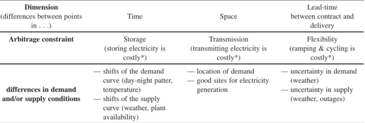
Table 1: The Heterogeneity of Electricity Along Three Dimensions
Dimension (differences between points
in . . .)
Time Space
Lead-time between contract and
delivery Arbitrage constraint Storage
(storing electricity is costly*) Transmission (transmitting electricity is costly*) Flexibility (ramping & cycling is
costly*)
differences in demand and/or supply conditions
— shifts of the demand curve (day-night patter, temperature)
— shifts of the supply curve (weather, plant availability)
— location of demand — good sites for electricity
generation
— uncertainty in demand (weather)
— uncertainty in supply (weather, outages)
* “Costly” both in the sense of losses (operational costs) and the opportunity costs of constraints.
Figure 2: The Marginal Value Spacev
Source: adopted from Hirth (2015a).
homogenous good. As physical constraints limit arbitrage, the marginal value varies along all three axes. This is, according to our definition, heterogeneity.
More formally, Figure 2 can be thought of as a [TxNxS]-Matrix where each element is an instantaneous marginal valuevt,n,⬘ s at time stept∈T, at noden∈N, and at lead-times∈S. We call the[TxNxS]-Matrixvof the elements v⬘t,n,s the “marginal value space”. Electricity is hetero-geneous because not all elements ofvare the same.
We are not the first, of course, to note that production-profile, location, and flexibility of power plants matter for economics. Dedicated power system models, such as stochastic security-constrained unit commitment models, implicitly take these factors into account. It is simple tools such as LCOE and grid parity, however, that shape much of the public debate.
5. Mean [range] prices for electricity were 44€/MWh [ – 222; + 210]; for natural gas 26€/MWh [21; 38]; for crude oil 114€/bbl [89; 130]. German spot prices from EPEX Spot, natural gas prices from German gas hub TTF, crude oil prices for Brent. Texas spot prices from ERCOT, German imbalance prices from TSO TenneT,
6. The German spot market EPEX clears for each quarter-hour of the year as a uniform price; the ERCOT real-time market of Texas clears every five minutes for each of all 10,000 bus bars of the system
Our formulation of three-dimensional heterogeneity provides an economic interpretation in terms of prices. To us, it seems to be a useful and general way of thinking about a wide range of economic issues in power generation, ranging from economic evaluation of power plant flexibility and forecast errors to congestion pricing and the costs of wind and solar intermittency. These topics are usually discussed separately; however, they can also be thought of as aspects of the three dimensional heterogeneity of electricity.
2.4 Observing Heterogeneity in the Power Sector
Three-dimensional heterogeneity is reflected in reality: through price variation, market design, and technology development. Take German price data from 2012 as an example. The range of electricity prices was 1000% of the mean electricity price, and prices varied by a factor of two during a normal day. The price of other energy carriers fluctuated much less: natural gas prices varied 70% of the mean price, and crude oil prices by 36% of their mean; neither commodity demonstrated within-day price variation.5This is in line with expectations, as storage costs for natural gas are higher than for oil, but much lower than for electricity. Price variation along the other dimensions can also be substantial. The spread between day-ahead and real-time price in Germany varied between -1600€/MWh and 1400€/MWh (Hirth & Ziegenhagen 2015); while the electricity price is uniform across Germany, in Texas price differences of several hundred $/MWh between different locations were not uncommon (Schumacher 2013). The peak load pricing liter-ature (Boiteux 1949, Crew et al. 1995) offers the theoretical foundations for equilibrium pricing of time-heterogeneous goods.
More structurally, heterogeneity is reflected in the design of whole power markets and market-clearing mechanisms. European power exchanges typically clear the market each hour in each bidding zone; U.S. markets often clear the market in steps of five minutes in each node of the transmission grid. Such high-frequency market clearing would be of no use without temporal het-erogeneity. Many spot markets feature a sequence of markets along lead-times, ranging from day-ahead to intra-day to real-time (or balancing) markets, sometimes called a “multi-settlement design”. Hence, there is notoneelectricity price per market and year, but 100,000 prices (in Germany) or three billion prices (in Texas).6Figure 2 can readily be thought of as an array of market-clearing spot prices with, in the case of Texas, three billion elements. Not all dimensions of heterogeneity are, however, reflected in all markets: German prices are uniform across space; grid constraints are managed via command and control instruments.
Heterogeneity of electricity has not only shaped market design, but also technology de-velopment. For homogenous goods, one single production technology is typically efficient. In elec-tricity generation, there is a set of generation technologies that are efficient (Bessiere 1970, Stough-ton et al. 1980, Grubb 1991, Stoft 2002). “Base load” plants have high investment, but low variable costs; this is reversed for “peak load” plants (Table 2). The latter are specialized in only delivering electricity at high prices, which rarely occurs. If electricity was a homogeneous good, no such technology differentiation would have emerged.
Table 2: Electricity Generation Technologies Have Adapted to Temporal Heterogeneity
Technology Annualized fixed costs
(€/kWa) Variable costs (€/MWh)
Least-cost technology for capacity factors of:
Nuclear 400 10 ⬎95%
Lignite 240 30 75%–95%
Hard coal 170 40 50%–75%
CCGT (natural gas) 100 55 5%–50%
OCGT (natural gas, oil) 60 140 ⬍5%
Cost data for central Europe with 2012 market prices for fuel, assuming a CO2price of 20€/t. About 85–90% of fixed costs are capital costs. CCGTs are combined-cycle gas turbines, and OCGTs are open-cycle gas turbines. Source for technology cost parameters: Hirth (2015a), based on the primary sources IEA & NEA (2010), VGB Powertech (2011), Black & Veatch (2012), and Schro¨der et al. (2013).
7. Throughout the paper, we restrict the analysis to first-order conditions, assuming well-behaved functions.
3. WELFARE ECONOMICS OF ELECTRICITY GENERATION: TECHNOLOGY PERSPECTIVE
This section derives the optimal generation mix. We formally derive the first-order con-ditions which explicitly account for three-dimensional heterogeneity. These concon-ditions can be in-terpreted such that each technology produces a different economic good. This section generalizes Joskow (2011) and formalizes Hirth et al. (2015).
3.1 Optimality Conditions: Marginal Benefit Equals Marginal Cost (for each technology)
The welfare-optimal quantityq∗ of any good is given by the intersection of the marginal economic value (benefit) of consuming the goodv⬘(q∗)and marginal economic cost of producing itc⬘(q):7
∗ ∗
v⬘(q ) =c⬘(q ) (3)
Throughout the paper, we will specify value and cost in energy terms ($/MWh). The long-term marginal cost of producing one MWh of electricity with technologyi,c⬘i, is the average discounted private life-cycle cost per unit of output (e.g., IEA & NEA 2010, Moomaw et al. 2011):
Y –y c (1 +r)
∑
y= 1 i,y c⬘i:= Y –y ∀i∈I (4) g (1 +r)∑
y= 1 i,ywhereci,y is the fixed and variable cost (including capital cost) that occurs in year y, gi,y is the amount of electricity generated in that year,ris the real discount rate, andYis the life-time of the asset in years. c⬘i is termed “levelized energy costs” (LEC) or “levelized costs of electricity” (LCOE). LCOE is a standard concept and broadly used.
8. The existence ofv⬘t,n,sdoes not require perfect and complete markets, nor equilibrium conditions. We add interpretation in terms of prices (which requires these assumptions) in brackets for convenience.
9. Assuming the optimal quantity of all technologies is positive. Otherwise the corresponding KKT-inequalities apply. 10. For example because they feature different variable costs, and hence are dispatched differently—or, because they are located at different sites, maybe because at some locations wind speeds are high while at others local coal resources are abundant.
T N S
v¯⬘i =
∑ ∑ ∑
gi,t,n,s⋅v⬘t,n,s ∀i∈I (5)t= 1n= 1s= 1
wherev⬘t,n,sis the instantaneous marginal value of electricity as defined in (1). This is the consumers’ willingness to pay for consuming one additional unit of electricity (MWh) at timet, noden, and lead-time s. We define T to be one year, N one power system, and S the complete set of spot markets.
Note that v⬘t,n,s does not carry a subscript for generation technology—this is a formal express of homogeneity (section 2a.
The weightsgi,t,n,sis the share of output of technologyiat the respective time step, node, and lead-time, such that
T N S
g = 1 ∀i∈I (6)
∑ ∑ ∑
i,t,n,st= 1n= 1s= 1
We label the [TxNxS]-Matrixgiof the elements gi,t,n,sthe “generation pattern” of technology i. Hence, the marginal value of a coal-fired plant,v¯⬘coal, is the average of the instantaneous value of electricity, weighted with the production pattern of coal plants. [Under perfect and complete mar-kets,v⬘ equals the locational spot price, andv¯⬘ equals the market value of a technology.]8
t,n,s i
TheIfirst order conditions for the optimal generation mix are:9
c⬘i =v¯⬘i ∀i∈I (7)
3.2 Interpretation: Different Generators Produce Different Goods
These equations look innocent, but provide a number of relevant interpretations. In general, the generation patterns of two technologies do not coincide .10
Hence, (gi≠gj)
their marginal value ($/MWh) does not coincide(v¯⬘i ≠v¯⬘j). The two technologies produce the same physical output (MWh of electricity), but they producedifferent economic goods.The value dif-ference shows that these “electricity goods” are only imperfectly substitutable.While at a single point (“instantaneously”), electricity from wind and coal is perfectly substitutable, over one year (more precisely, over the full value space), it is not. The law of one price doesnotapply (Figure 3). Optimality condition (4) actually represents Ioptimality conditions for I different electricity goods, corresponding toIgeneration technologies. Expressing optimality in this way might hence be called a “technology perspective”.
4. WELFARE ECONOMICS OF ELECTRICITY GENERATION REFORMULATED: LOAD PERSPECTIVE
The previous section derived first-order conditions for the optimal generation mix as the equality of marginal costs and marginal benefits of each electricity good. This section derives an
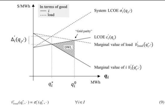
Figure 3: LCOE and Marginal Value in the Long-Term Optimum
In the long-term optimum, the marginal value of each technology coincides with the marginal cost of that technology— but, in general, it does not coincide with the marginal value of any other technology (levels are illustrative). “Load” will be discussed below.
alternative formulation of the same optimality conditions in terms ofthe sameelectricity good, i.e. a “reference good”. One can think of “transforming” the output of each generator into the same good (the “transformation” is analytical, not physical). This perspective is mathematically equiva-lent, but offers a number of interpretations that will turn out helpful for deriving an alternative cost metric to LCOE.
4.1 Choosing “Load” as a Reference Electricity Good
As a reference electricity good, we choose “load”(l), defined as a MWh of electricity that has the pattern of electricity consumption. The matrixl, defined analogously to the “generation pattern”gi(6), consists of elementslt,n,sthat represent the share of consumption at the respective time-step, node, and lead time. The elements sum up to unity. The simplest way to supply this electricity good can be imagined as a (hypothetical) “ideal” generator that follows load over time, has the same spatial distribution as load, and forecast errors perfectly correlated to load.
Accordingly, we define the marginal value of loadv¯⬘load as the demand-weighted average of allv⬘t,n,s:
T N S
v¯⬘load=
∑ ∑ ∑
lt,n,s⋅v⬘t,n,s (8)t= 1n= 1s= 1
is the consumers’ willingness to pay for an additional MWh of yearly electricity consumption,
v¯⬘load
assuming that it has the same pattern as infra-marginal consumption. [Under perfect and complete markets,v¯⬘load equals the average wholesale electricity prices consumers pay,p¯⬘load.]
4.2 Optimality Conditions from a Load-perspective
Now we reformulate the optimality conditions (7). Optimally, the marginal benefit of the good loadv¯⬘load coincides with the marginal cost of producing this good by technologyi:
Figure 4: Optimal Quantityq∗i of Technologyiin Terms of the Good i (Technology Perspective) and Load (Load Perspective)
∗ ∗
v¯load⬘ (qi,⋅) =σ⬘i(qi,⋅) ∀i∈I (9)
We termσ⬘i “System LCOE” and define it to be the sum of generation costsc⬘i and the costs of “transforming” the electricity good,D⬘i:
σi⬘(qi,⋅) :=c⬘i(qi) +D⬘i(qi,⋅) ∀i∈I (10) Ueckerdt et al. (2013a) show thatD⬘i is the increase in system costs as generation from technology
iis increased. Below we show that it can also be interpreted as a “value gap”. Whilec⬘i is strictly positive,D⬘i can be of either sign.
Note that c⬘i, is a function ofqionly, but σ⬘i andD⬘i are functions of other arguments as well, including power system parameters and the plant mix, just asv¯⬘i. This reflects the fact that in a (power) system, cost-benefit analysis cannot be done for individual parts of the system such as one technology in isolation.
This set ofIfirst-order conditions can be expressed as equalities of System LCOE:
∗ ∗
σi⬘(qi,⋅) =σ⬘j(qj,⋅) ∀i,j∈I (11)
The first-order condition for the optimal quantityq∗i can be written in two ways. First, in terms of the electricity good that corresponds to the technology i(equation 7), and second, in terms of a reference electricity good (equation 9). Figure 4 illustrates this duality graphically. The “technology perspective” is depicted in bold lines. The intersection of marginal costs (LCOE) and marginal value ofiindicates the optimal quantityq∗i. The “load perspective” is drawn in dotted lines. The intersection of marginal costs (System LCOE) and marginal value of load results in the same quantity q∗. Ignoring variability leads to the sub-optimal quantity q0, with corresponding
dead-i i
4.3 Four Interpretations ofD⬘i
can be interpreted in at least four different ways. First, it can be understood as the costs D⬘i
of transforming output from a technology to serve load. These costs not only depend on the gen-eration pattern of the technology but also on properties of the rest of the power system. Hence, the additional costs might be calledsystem-level costs(or system costs), which has inspired us to coin the term “System LCOE”.
Second, we can reformulate (10), using (9) and (7), to derive
∗ ∗ ∗
Di⬘(qi,⋅) =v¯⬘load(qi,⋅) –v¯⬘i(qi,⋅) ∀i∈I (12) is thevalue gapbetween the value of electricity that consumers demand and the value of
D⬘i v¯⬘load
electricity that a certain generator supplies,v¯⬘i. Comparingσ⬘i of two technologies means simul-taneously comparingbothcost and value differences.
Third, one might callD⬘i variability cost. The value difference between technologies is determined by the deviations of the generation pattern of a technology from the load pattern. We interpret this mismatch as variability of that technology andD⬘i as opportunity cost of variability. It follows that all generators, not just VRE, are subject to variability and associated costs. More fundamentally, it is the combination of electricity being heterogeneous (not all elements ofvare the same) and power plant variability (gi≠l) that causes a value gap to emerge (v¯i⬘≠v¯⬘load). If electricity was either homogeneous or generation was not variable it would hold that v¯⬘i =
.
v¯⬘load ∀i∈I
Fourth,D⬘i can be interpreted asintegration costs. There is a large branch of literature that assesses the impact of wind and solar variability in terms of “integration costs” when integrating VRE generators into power systems (e.g. Dragon & Milligan 2003, Sims et al. 2011, Holttinen et al. 2011, Milligan et al. 2011, NEA 2012, Baker et al. 2013, IEA 2014). These studies often calculate different items, such as balancing, grid, and adequacy costs. It is unclear how the sum of these items can be interpreted economically. Milligan et al. (2013) report that readers “add the integration cost to the cost of energy from wind power to provide a comparison of wind energy to a more dispatchable technology”. Presumably readers do this to assess competitiveness and efficiency; therefore we believe it is sensible to define integration costs asD⬘i, which allows such an assessment (Ueckerdt et al. 2013a, Hirth et al. 2015). According to this definition, integration costs are not specific to VRE.
The two perspectives of sections 3 and 4—technologyandload—correspond to two equiv-alent ways of accounting for the economic consequences of wind and solar power intermittency. In one perspective, intermittency leads to a reduction of the valuev¯⬘i of a technology compared to the average wholesale electricity pricev¯⬘load. In the other perspective, system costs are added to generation costs of the technology. Some analysts find one perspective more intuitive and appealing, while others prefer the other. Energy traders and economists often prefer to think of variability decreasing the value of wind and solar power. They often find the “technology perspective” to be quite natural. System operators, policy makers, modelers, and power system engineers often strive to understand the cost of variability and hence prefer the “load perspective”.
In the remainder of this paper we callD⬘i system costs.
4.4 Why LCOE-comparisons, Grid Parity, and IAMs Can Be Problematic
The fact that each generation technology produces output of different value has important implications for the interpretation of metrics and tools that are commonly used to assess power
Figure 5: LCOE, Variability Costs, and System LCOE in the Long-term Economic Equilibrium (levels are illustrative)
11. Comparing LCOE is meaningful if generators produce comparable output. If, say, nuclear power and lignite plants have similarly low variable costs and are consequently dispatched similarly, are both located similarly far from load centers, and are similarly inflexible, comparing costs is sufficient to determine relative competitiveness.
12. Furthermore, “grid parity” conceals the fact that grid fees, levies, taxes comprise a large share of retail prices. Hence it takes a private perspective that has little implication for social efficiency (Hirth 2015b).
generating technologies: comparisons of LCOE, grid parity, and macroeconomic multi-sector mod-els. All three approaches have in common that, if not carefully used, they ignore value differences and can deliver biased results.
It is common practice in policy and industry documents (and also in academic articles) to compare the LCOE of different technologies (Karlynn & Schwabe 2009, Fischedick et al. 2011, IEA & NEA 2010, BSW 2011, EPIA 2011, Nitsch et al. 2010, IRENA 2012, GEA 2012, EIA 2013, DECC 2013, IRENA 2015). Authors and readers apparently appreciate the straightforward interpretation that LCOE seems to allow. Many readers interpret cost advantage as a sign of effi-ciency or competitiveness. Such reasoning would be correct if and only if, the value of output of all generators was identical—which is not the case. In fact, comparing LCOE from different tech-nologies is comparing the marginal costs of producing different goods.11
If power generating technologies are to be compared economically along a single axis, System LCOE could be used. The optimality conditions (12) imply that System LCOE from dif-ferent technologies can be compared to infer about efficiency of each technology. Figure 5 illustrates the long-term optimum: while LCOE of different technologies do not coincide, System LCOE do. Some studies seem to suggest that once a technology has reached “grid parity”, its de-ployment is economically efficient (BSW 2011, EPIA 2011, Koch 2013, Fraunhofer ISE 2013, Breyer & Gerlach 2013). Grid parity is usually defined as the point where LCOE of solar (or wind) power fall below the retail electricity price. Again, this indicator ignores heterogeneity, and im-plicitly compares the marginal value of one good (v¯⬘load) with the marginal cost of a different good
.12 Comparing a technology’s LCOE to the wholesale electricity price (Kost et al. 2012, (c⬘solar)
Clover 2013, Ru¨diger & Matieu 2014) is based on the same flawed implicit assumption.
Ignoring value differences among generation technologies introduces a bias: it makes low-value technologies look better than they actually are, biasing their optimal/equilibrium market share upwards. This systematically favors conventional base-load generators relative to peak-load gen-erators (“base load bias”), and, at high penetration rates, wind and solar power relative to dispatch-able generators (“VRE bias”, for quantitative evidence see section 0). Simple macroeconomic mod-els can be subject to this bias as well.
Economists have used calibrated multi-sector models for many years for research and policy advice (Leontief 1941, Johansen 1960, Taylor & Black 1974). Today, “integrated assessment models” (IAMs), sometimes based on computable general equilibrium (CGE) models, are an im-portant tool for assessing climate policy and the role of renewables in mitigating greenhouse gas emissions (Fischedick et al. 2011, Edenhofer et al. 2013, Luderer et al. 2014, Knopf et al. 2013, IPCC 2014).
Large-scale models are applied to account for macroeconomic effects, endogenously model fuel prices and energy demand, and incorporate endogenous technological learning. These capa-bilities, however, come at the price of coarse resolution. The typical time resolution of IAMs is 5– 10 years and model regions are of continental scale. Due to numerical constraints, IAMs cannot provide the temporal and spatial resolution required to explicitly represent the heterogeneity of electricity. When optimizing the generation mix, old versions of such models implicitly equate the marginal costs of different goods.
Accounting for heterogeneity and thus accounting for the impacts of variability is a major challenge to IAM modeling (Luderer et al. 2014, Baker et al. 2013). While all generators are subject to variability, we focus here on VRE, because there is a rich academic debate around them. Many models use stylized formulations to account for variability, however, most of these approaches lack welfare-theoretical rigor. While some models—mostly older versions—ignore variability altogether and thus generate results that are biased towards optimistic cost estimates, today most IAMs apply some sort of stylized formulation to represent the challenges of variability. Of the 17 models re-viewed by Luderer et al. (2014), two ignore variability; the others limit the maximum share of variable renewables (seven models), require dedicated storage or back-up capacity (eight models), or add a cost penalty (four models: MERGE, MESSAGE, ReMIND, and WITCH). The most basic approach is to set a hard limit to the generation share of wind and solar. However, this implicitly assumes zero marginal value at higher shares and ignore the possibility for system adjustments even under strong economic pressure. A more economic approach is to introduce an “integration cost penalty” that might increase with its penetration. Other models require the provision of specific technology options to foster the integration of VRE, like gas-fired backup capacities or electricity storage. Six models represent load variability with a load duration curve. Sullivan et al. (2013) propose a “flexibility constraint” to account for variability. However, all these approaches have three limitations. First, the foundations and completeness of the approaches is unclear. Often mo-tivated from a technical perspective, they lack a clear relation to the economic costs of variability. Second, each approach focuses on specific aspects of variability while omitting others. Finally, these stylized representations are difficult to parameterize.
System LCOE offers a pathway of how the electricity sector could be modeled in IAMs. It contains variability costs, which serve as cost penalties that account for all aspects of variability on a rigorous economic basis. Not only wind and solar power, but all generation technologies are associated with such costs and should therefore be represented by their System LCOE. To estimate
13. Multi-sector models that capture important issues such as learning curves or macroeconomic effects often need to reduce power system detail to remain numerically feasible.
variability costs, tools other than IAMs are needed, such as high-resolution numerical power system models. To keep this parameterization manageable, it should focus on the most important aspects of variability. Implementing System LCOE can be combined with other more explicit approaches of representing variability. Those aspects that can be directly represented could be exempt from the System LCOE metric. For example, an explicit representation of residual load duration curves can be complemented with parameterizations of grid and balancing costs (Ueckerdt et al. 2014). The following section suggests approaches of how to estimate the necessary parameter values.
5. EMPIRICALLY ESTIMATING VARIABILITY COSTS: PRAGMATIC IDEAS
For long-term planning, policy and investment decisions, governments, utilities, and sys-tem operators might want to estimate the optimal generation mix for the future. The first-order conditions (7) and (9) assume complete information—specifically, full knowledge about the mar-ginal value spacev. In reality, information is often far from complete. This section suggests how to estimate system costs empirically under incomplete information. It proposes splitting system costs into three “cost components” and shows how they can be estimated from existing power sector models and observed market data. We hope thereby to provide a pragmatic and feasible approach to estimate system costs.
Cost components might be useful for three reasons: to reduce complexity and improve understanding; to use piece-wise evidence; to use market data for estimation.
5.1 Decomposition—the Three Components of System Costs
Many published studies estimate the impact ofonedimension of heterogeneity (e.g. “the costs of wind forecast errors”). Such studies are often based on models that represent one dimension of variability (much) better than others. “Super models” that represents all three dimensions in full detail are rare: the best stochastic security-constrained unit commitment models might come close to this ideal, but in practice many studies rely on much less sophisticated tools.13Not only models are incomplete, the same is true for markets. For example, transmission constraints are not priced in most European markets. Given such incomplete knowledge about the marginal value spacev, we propose a pragmatic approximation: estimating the impact of each dimension of heterogeneity separately as one “cost component” and adding them up.
• The impact of time is called “profile costs” (because the temporal generation profile deter-mines its size).
• The impact of space is called “grid costs” (because grid constraints determine its size). • The impact of lead-time is called “balancing costs” (because forecast errors need to be
bal-anced).
We use the sum of the three components as an estimatorDˆ⬘i of the cost of variability: profile grid balancing
ˆ
is only an approximation of the system costs . The three cost components interact with each ˆ
D⬘i D⬘i
other such that there is an (unknown) interaction term. Policy that reduces one cost component might increase another.
When there is only information about the temporal structure of the marginal value of electricity,v⬘t,n,s reduces tov⬘t. We define profile costs as the difference between the load-weighted and the generation-weighted marginal value:
T profile
Di :=
∑
(lt–gi,t)⋅v⬘t ∀i∈I (14)t= 1
We define grid costs and balancing costs accordingly: N grid Di :=
∑
(ln–gi,n)⋅vn⬘ ∀i∈I (15) n= 1 S balancing Di :=∑
(ls–gi,s)⋅vs⬘ ∀i∈I (16) s= 1Note that all cost components all defined in marginal terms, asv⬘is the marginal value of electricity; all components can be positive or negative; all components are different for different technologies. Even if a “super model” is available that captures all three dimensions appropriately, these three “cost components” might provide a helpful way of post-processing and interpreting model results. The Appendix provides further discussion on the interaction term and an example calculation of the cost components.
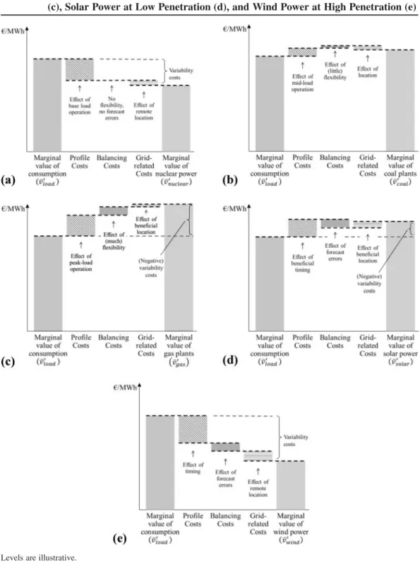
The waterfall diagrams of Figure 6 illustrate the three cost components for different tech-nologies. Base load generators such as nuclear power (a) have a lower value than the marginal value of consumption (v¯⬘load), while mid-load generators such as coal-fired plants (b) have a value that is similar tov¯⬘load. The inflexibility of these generators reduces their value. Peak-load generators such as gas-fired plants (c) have a higher value, because they produce disproportionally during times of high prices, are located closer to load centers, and can provide short-term flexibility— hence all cost components increase their marginal value. The value of VRE is strongly affected by their penetration. At low penetration, their value is typically higher than the marginal value of consumption, especially in the case of solar power (d): the benefits of producing during times of high prices outweigh the costs of forecast errors. At high penetration, profile, balancing, and grid related costs tend to reduce the value of solar as well as of wind power (e).
The three cost components, profile, balancing, and grid costs, are not constant parameters, but functions of many system properties. They typically increase with penetration, as illustrated in Figure 7.
5.2 Market- and Model-based Estimation
Each cost component can be estimated from modeled shadow prices or from observed market prices. Table 3 lists the markets and models that can provide information regarding each cost component. Take the example of grid costs: they can be estimated from locational shadow prices derived from grid models, or from empirically observed nodal prices. Where such prices do not exist, zonal prices and locational differentiated grid fees can serve as proxies.
Figure 6: The Marginal Value of Nuclear Power (a), Coal-fired Plants (b), Gas-fired Plants (c), Solar Power at Low Penetration (d), and Wind Power at High Penetration (e)
Figure 7: Profile, Balancing, and Grid Costs Typically Increase with Penetration
For wind and solar power, profile costs are often negative at low penetration.
Table 3: Estimating Cost Components from Markets and Models
Models Markets
Profile costs power market models day-ahead spot markets
Balancing costs stochastic unit commitment models real-time spot markets; balancing power / imbalance markets
Grid costs (optimal) power flow models / grid models
locational (nodal, zonal) spot markets; locational grid fees
Both markets and models have limitations: markets are never complete and free of market failures. Power markets can be off the equilibrium for extended periods of time, given the long life-time of assets. In some markets (e.g. many balancing markets), regulators have implemented average, not marginal, pricing. In other markets (e.g. many grids), costs are socialized altogether.
Models, in turn, are necessarily simplifications of reality: externalities are often incom-pletely captured, and some models do not estimate the long-term equilibrium. In addition, numerical models are often calibrated to historical market prices, and might hence be subject to the same limitations as markets. While both sources of empirical data are imperfect, diversified estimation methodology helps derive robust estimates.
6. WHAT IS SPECIAL ABOUT WIND AND SOLAR POWER?
When we began writing this paper, we were looking for the fundamental economic dif-ferences between VRE and other generators—“the economics of intermittency”—in order to pa-rameterize “integration costs” in multi-sector models. The previous literature had identified three specific properties of VRE: fluctuations, forecast errors, and the fact that good sites are often far from load centers (GE Energy 2010, Milligan et al. 2011, Borenstein 2012, IEA 2014).
However, as shown above, these properties are not limited to wind and solar power. It is true that the generation patterns in time, space, and lead-time affect the economic value of electricity generated from wind and solar power—but that is true for all generation technologies! It is true that using LCOE comparisons, grid parity, or simple multi-sector models to compare VRE with
Table 4: Quantitative Literature on Integration Costs of Wind Power
Models Markets
Profile costs Grubb (1991), Rahman & Bouzguenda (1994), Rahman (1990), Bouzguenda & Rahman (1993), Hirst & Hild (2004), ISET et al. (2008), Braun et al. (2008), Obersteiner & Saguan (2010), Obersteiner et al. (2009), Boccard (2010), Green & Vasilakos (2011), Energy Brainpool (2011), Valenzuela & Wang (2011), Martin & Diesendorf (1983), Swider & Weber (2006), Lamont (2008), Bushnell (2010), Gowrisankaran et al. (2011), Mills & Wiser (2012, 2014), Mills (2011), Nicolosi (2012), Kopp et al. (2012), Hirth (2013, 2015b), Bolkesjø et al. (2014), Hirth & Mu¨ller (2015)
Borenstein (2008), Sensfuß (2007), Sensfuß & Ragwitz (2011), Fripp & Wiser (2008), Brown & Rowlands (2009), Lewis (2010), Green & Vasilakos (2012), Hirth (2013)
Balancing costs Grubb (1991), Gross et al. (2006), Strbac et al. (2007), Smith et al. (2007), DeMeo et al. (2007), Mills & Wiser (2012, 2013, 2014), Gowrisankaran et al. (2011), Carlsson (2011), Holttinen et al. (2011), Garrigle & Leahy (2013), Pudjianto et al. (2013)
Holttinen (2005), Pinson et al. (2007), Obersteiner et al. (2010), Holttinen & Koreneff (2012), Katzenstein & Apt (2012), Louma et al. (2014), e3 consult (2014), Hirth et al. (2015)
Grid costs Strbac et al. (2007), Denny & O’Malley (2007), dena (2010), Holttinen et al. (2011), NREL (2012), Pudjianto et al. (2013), E-Bridge et al. (2014), 50Hertz et al. (2014)
Hamidi et al. (2011), Schumacher (2013), Brown and Rowlands (2009), Lewis (2010), Hirth et al. (2015)
dispatchable generators introduces a bias—but the comparison among dispatchable technologies is also biased.
Based on economic reasoning, it seems hard to support the proposition that one group of (“intermittent”) generators that is qualitatively distinct from another group of (“dispatchable”) gen-erators. Rather, electricity itself that is different from other economic goods, and each electricity-producing technology has particular properties. So—are wind and solar power just two more power generation technologies?
What isspecial about wind and solar power is not the existence, but thesize of system costs. In predominantly thermal power systems, at high penetration rates (such as 20 + % for wind or 10 + % for solar in annual energy terms), they are the technologies that produce least-value electricity. In other words, ignoring value differences can bias the assessment of all generators, but the upward bias might be greatest for wind and solar power. In the following, we present results from a quantitative literature review of wind power system costs that produced this finding (updated from Hirth et al. 2015).
Table 4 lists all studies we are aware of that can be used to extract wind variability cost estimates. With a few exceptions (notably Grubb 1991, Holttinen et al. 2011, and Mills & Wiser 2012), most of these studies report estimates of one single cost component.
Figure 8 and Figure 9 summarize estimates of profile costs and balancing costs that we extracted from these studies. Profile costs are estimated to be⬃20€/MWh at 30–40% penetration; many studies find negative costs at low penetration (implying a higher price received at spot markets than the load-weighted price). Balancing costs are estimated to rise from ⬃2€/MWh at low pen-etration to ⬃4 €/MWh at high penetration. Grid costs (not in figure) are likely to be below 15 €/MWh under most conditions (Hirth & Mu¨ller 2015).
The most important finding of the literature review is that system costs can become very high at high penetration rates. When wind penetration reaches 30–40%, they seem to be in the
Figure 8: Wind Profile Cost Estimates for Thermal Power Systems
Estimates extracted from about 30 published studies. Studies are differentiated by how they determine electricity prices: from markets (squares), from short-term dispatch modeling (diamonds, dotted line), or from long-term dispatch and in-vestment modeling (triangles, bold line). To improve comparability, the system base price has been normalized to 70€/ MWh in all the studies. Updated from Hirth et al. (2015).
Figure 9: Wind Balancing Cost Estimates for Thermal Power Systems
Estimates extracted from about 20 published studies based on market prices (squares) or models (diamonds, dotted line). Three market-based studies report very high balancing costs, but these are unlikely to reflect marginal costs. All other estimates are below 6€/MWh. Studies of hydro-dominated systems show very low balancing costs (triangles). Updated from Hirth et al. (2015).
range of 25–35 €/MWh, assuming an average electricity price of 70 €/MWh. In other words, electricity from wind power is worth only 35–45€/MWh under those conditions, 35–50% less than the average electricity price. If wind LCOE are 60€/MWh, system (variability) costs are ⬃50% of generation costs.
However, the literature also shows that system costs are low, or even negative, at low penetration rates. Up to 10% penetration rate, system costs are most likely to be small relative to generation costs.
Four additional findings can be identified: (i) costs increase with penetration; (ii) at high penetration, profile costs are higher than balancing costs; (iii) long-term models (with endogenous investment) report lower profile costs than short-term models; (iv) costs are lower in hydro-domi-nated systems than in thermal systems.
Positive system costs imply that optimal deployment is lower than it would be otherwise— but it is not necessarily low in absolute terms. Even IAMs that attach significant integration costs to wind power often find high renewable shares under strict climate policy. The same is true for power market models: Neuhoff et al. (2008) reports an optimal wind share for the UK of 40%. Hirth (2015a) finds an optimal wind share of 20% [1–45%], roughly in line with Lamont (2008). Mu¨sgens (2013) and Eurelectric (2013) reports an optimal wind share in Europe of more than one third by 2050.
7. CONCLUDING REMARKS
This paper has taken a micro-economic perspective on electricity generation. We have shown that electricity is a heterogeneous economic good and that, consequently, cost comparisons and multi-sector models have to be used with care. We hope this serves modelers as well as those who advise decision makers based on such tools.
We have argued that electricity is a paradoxical economic good: it can be understood as being perfectly homogenous, and as very heterogeneous. Electricity prices vary over time, across space, and with respect to lead-time between contract and delivery. As a consequence, the economic value of electricity generated from different power plant technologies diverges. Physically, they all produce megawatt-hours of electricity; economically, they produce different goods. Common tools to evaluate generation technologies—LCOE, grid parity, (simple) multi-sector models—account for cost differences among generation technologies, but ignore these value differences. They implicitly equate marginal costs and benefits of different goods. Ignoring value differences introduces two biases: the “base-load bias” and the “VRE bias”. VRE generators, such as wind and solar power, produce particularly low-value electricity if deployed at large scale, hence the upward bias is par-ticular strong. System planning based on biased analyses will lead to a sub-optimal plant mix and corresponding welfare losses.
This leads us to threemethodological conclusions. First, when comparing the economics of power generation technologies in a one-dimensional figure, System LCOE should be used instead of LCOE. System LCOE accounts for both value and cost differences; the metric can be interpreted as the cost of each generation technology to produce the same good. Second, multi-sector models, such as integrated assessment models or general equilibrium models, need to carefully account for value differences among generation technologies. This is especially relevant if they are used to model structural shifts in electricity supply such as deep decarbonization of the power sector. Finally, grid parity is not a useful indicator for the economic efficiency of generation technologies. We recommend that it is not used.
The most importantpolicy conclusionof this assessment might be that there is none. In principle, markets are well equipped to price heterogeneity. Neither electricity heterogeneity nor wind and solar variability constitutes an externality, and there is no need for policy interventions. Looking closer to real-word markets, the situation is less black and white. More than in other sectors, governments and regulators shape the design of electricity markets. In in many markets, electricity prices variation are suppressed by the way markets are designed. For example, in many European markets, regulators mandate geographically uniform prices. Often, balancing prices do not reflect marginal, but average, costs. The findings of this article imply that policy should allow electricity prices to vary along all three dimensions of heterogeneity. They should do so at the level of wholesale markets, retail markets, and policy instruments—subject to the transaction cost trade-off. Specifically, renewable support schemes should be permeable for price signals in the sense that they should transmit price variations to investors. Simple feed-in-tariffs eliminate all price vari-ability.
Finally, this paper might also offer afundamental interpretation of the nature of power generating technologies. It shows that wind and solar are not that different from other generators in the end. It is indeed questionable if it is sensible to draw a line between “variable” and “dis-patchable” generators. Each generation technology has specific characteristics and produces output of a different value in $/MWh terms. Accounting for these value differences is important when assessing wind and solar power—but it is equally important when assessing other technologies.
ACKNOWLEDGMENTS
We would like to thank Michael Pahle, Brigitte Knopf, Eva Schmid, Dick Schmalensee, Meike Riebau, Mats Nilsson, Simon Mu¨ller, Robert Pietzcker, Gunnar Luderer, Michele Peruzzi, Wolf-Peter Schill, and Catrin Jung-Draschil for inspiring discussions and three anonymous referees for helpful comments. All remaining errors are ours. The findings, interpretations, and conclusions expressed herein are those of the authors and do not necessarily reflect the views of their respective institutions. An earlier version of this article has been published as FEEM Working Paper 2014.039.
APPENDIX Interaction Term
is only an approximation of the system costs . The three cost components interact ˆ
D⬘i D⬘i
with each other and there is an (unknown) interaction termφˆi.
ˆ ˆ
D⬘i =D⬘i +φi ∀i∈I (17)
However, lacking knowledge of the sign of the interaction, we believe settingφˆito zero is a sensible first-order approximation.
Example Calculation
As an illustrative example, assume one needs to assess the marginal value of wind power in Germany at some point in the future. Say, there is a power market model available that delivers estimates for the marginal value of load of 70€/MWh and of wind power of 60€/MWh, but that model does not capture the grid, nor does it capture uncertainty—hence does not account for the
14. Grid costs are the spread between the load-weighted and the wind-weighted electricity price:12 6– = 2 3 3
second and the third dimension of heterogeneity. From a literature review, one estimates balancing costs (the cost of wind forecast errors) to be 3€/MWh. Finally, a grid study reports the marginal value of electricity in Northern Germany to be 6€/MWh higher in the South than in the North, and it is known that two thirds of all turbines are located in the North while two thirds of con-sumption is in the South. Hence, profile costs are 10€/MWh, balancing costs 3€/MWh, and grid costs 2€/MWh.14In sum, the marginal value of wind power isv¯ˆ⬘
wind= 55€/MWh, and the variability cost of wind powerDˆ⬘wind= 15€/MWh.
REFERENCES
50Hertz Transmission GmbH, Amprion GmbH, TennT TSO GmbH & TransnetBW GmbH (2014):Netzentwicklungsplan Strom 2014, Zweiter Entwurf, www.netzentwicklungsplan.de.
Baker, Erin, Meredith Fowlie Derek Lemoine and Stanley Reynolds (2013): “The Economics of Solar Electricity,”Annual Review of Resource Economics5. http://dx.doi.org/10.1146/annurev-resource-091912-151843.
Bessembinder, Hendrik and Michael Lemmon (2002): “Equilibrium Pricing and Optimal Hedging in Electricity Forward Markets,”The Journal of FinanceLVII(3), 1347–1382. http://dx.doi.org/10.1111/1540-6261.00463.
Bessiere, F. (1970): “The investment 85 model of Electricite de France,”Management Science17 (4), B-192–B-211. http:// dx.doi.org/10.1287/mnsc.17.4.B192.
Black and Veatch (2012):Cost and Performance Data for Power Generation Technologies. Prepared for the National Renewable Energy Laboratory.
Boccard, Nicolas (2010): “Economic properties of wind power. A European assessment,”Energy Policy38: 3232–3244. http://dx.doi.org/10.1016/j.enpol.2009.07.033.
Boiteux, Marcel (1949): “Peak-Load Pricing,” reprint (1960)The Journal of Business33(2), 157–179. http://dx.doi.org/ 10.1086/294331.
Borenstein, Severin (2008): “The Market Value and Cost of Solar Photovoltaic Electricity Production,”CSEM Working Paper176.
Borenstein, Severin (2012): “The Private and Public Economics of Renewable Electricity Generation,”Journal of Economic Perspectives26(1): 67–92. http://dx.doi.org/10.1257/jep.26.1.67.
Bouzguenda, Mounir and Saifur Rahman (1993): “Value Analysis of Intermittent Generation Sources from the System Operator Perspective,”IEEE Transactions on Energy Conversion8(3): 484–490. http://dx.doi.org/10.1109/60.257063. Braun, Martin, Stefan Bofinger, Thomas Degner, Thomas Glotzbach and Yves-Marie Saint-Drenan (2008): “Value of PV
in Germany. Benefit from the substitution of conventional power plants and local power Generation,”Proceedings of the 23rd European Photovoltaic Solar Energy Conference, Sevilla.
Breyer, Christian and Alexander Gerlach (2013): “Global overview on grid-parity,”Progress in photovoltaics21(1): 121– 136. http://dx.doi.org/10.1002/pip.1254.
Brown, Sarah and Ian Rowlands (2009): “Nodal pricing in Ontario, Canada: Implications for solar PV electricity,”Renewable Energy34: 170–178. http://dx.doi.org/10.1016/j.renene.2008.02.029.
BSW (2011):Solarenergie wird wettbewerbsfa¨hig, Bundesverband Solarwirtschaft, www.solarwirtschaft.de/fileadmin/me-dia/pdf/anzeige1_bsw_energiewende.pdf.
Bushnell, James (2010): “Building Blocks: Investment in Renewable and Non-Renewable Technologies,” in: Boaz Moselle, Jorge Padilla and Richard Schmalensee:Harnessing Renewable Energy in Electric Power Systems: Theory, Practice, Policy, Washington.
Carlsson, Fredrik and (2011): “Wind power forecast errors. Future volumes and costs,”Elforsk report11:01. Clover, Robert (2013): “Energy Mix In Europe to 2050,”paper presented at the 2013 EWEA conference, Vienna. Covarrubias, A (1979): “Expansion Planning for Electric Power Systems,”IAEA Bulleting21(2/3): 55–64.
Crew, Michael, Chitru Fernando and Paul Kleindorfer (1995): “The Theory of Peak-Load Pricing. A Survey,”Journal of Regulatory Economics8: 215–248. http://dx.doi.org/10.1007/BF01070807.
DeMeo, Edgar, Gary Jordan, Clint Kalich, Jack King, Michael Milligan, Cliff Murley, Brett Oakleaf and Matthew Schuerger (2007): “Accomodating Wind”s Natural Behavior,”IEEE power & energy magazineNovember/December 2007. dena (2010):Netzstudie II—Integration erneuerbarer Energien in die deutsche Stromversorgung im Zeitraum 2015–2020
mit Ausblick 2025, Deutschen Energie-Agentur GmbH, Berlin.
Denny, Eleanor and Mark O’Malley (2007): “Quantifying the Total Net Benefits of Grid Integrated Wind,”IEEE Trans-actions on Power Systems22(2): 605–615. http://dx.doi.org/10.1109/TPWRS.2007.894864.
Dragon, Ken and Michael Milligan (2003): “Assessing Wind Integration Costs with Dispatch Models: A Case Study of PacifiCorp,”NREL Conference PaperCP-500-34022.
e3 consult (2014):“ Ausgleichsenergiekosten der Oekostrombilanzgruppe fuer Windkraftanlagen Endfassung,“Study for Interessengemeinschaft Windkraft O¨ sterreich, https://www.igwindkraft.at/mmedia/download/2014.05.21/140070419170 3835.pdf.
E-Bridge, IAEW and Offis (2014):Moderne Verteilernetze fu¨r Deutschland, report for Bundesministeriums fu¨r Wirtschaft und Energie (BMWi), Berlin.
Edenhofer, Ottmar, Lion Hirth, Brigitte Knopf, Michael Pahle, Steffen Schloemer, Eva Schmid and Falko Ueckerdt (2013): “On the Economics of Renewable Energy Sources,” Energy Economics 40(S1): 12–23. http://dx.doi.org/10.1016/ j.eneco.2013.09.015.
EIA (2013):Annual Energy Outlook 2013, U.S. Energy Information Administration.
Energy Brainpool (2011):Ermittlung des Marktwertes der deutschlandweiten Stromerzeugung aus regenerativen Kraftwer-ken, www.eeg-kwk.net/de/file/110801_Marktwertfaktoren.pdf.
EPIA (2011): Solar Photovoltaics competing in the energy sector, European Photovoltaic Industry Association, www.epia.org/news/publications/
Eurelectric (2013).PowerChoices Reloaded, Brussels.
Fischedick, M., R. Schaeffer, A. Adedoyin, M. Akai, T. Bruckner, L. Clarke, V. Krey, I. Savolainen, S. Teske, D. U¨ rge-Vorsatz and R. Wright (2011): „Mitigation Potential and Costs“, in: O. Edenhofer, R. Pichs-Madruga, Y. Sokona, K. Seyboth, P. Matschoss, S. Kadner, T. Zwickel, P. Eickemeier, G. Hansen, S. Schlo¨mer and C. v. Stechow (Eds.):IPCC Special Report on Renewable Energy Sources and Climate Change Mitigation,Cambridge University Press, Cambridge, UK. http://dx.doi.org/10.1017/CBO9781139151153.014.
Fraunhofer ISE (2013):Photovoltaics report, Fraunhofer Institute for Solar Energy Systems, www.ise.fraunhofer.de/mwg-internal/de5fs23hu73ds/progress?id = 94T8LFoGsA&dl.
Fripp, Matthias and Ryan H. Wiser (2008): “Effects of Temporal Wind Patterns in the value of wind-generated Electricity in California and the Northwest,” IEEE Transactions on Power Systems 23(2): 477–485. http://dx.doi.org/10.1109/ TPWRS.2008.919427.
Garrigle, E and E Leahy (2013): “The value of accuracy in wind energy forecasts,”Proceedings of the 12thInternational
Conference on Environment and Electrical Engineering,Wroclaw.
GE Energy (2010): “Western Wind and Solar Integration Study,”NREL Subcontract ReportSR-550-47434.
GEA (2012):Global Energy Assessment—Toward a Sustainable Future, Cambridge University Press, Cambridge, UK. Gowrisankaran, Gautam, Stanley S. Reynolds and Mario Samano (2011): “Intermittency and the Value of Renewable
Energy,”NBER Working Paper17086
Green, Richard (2005): “Electricity and Markets,”Oxford Review of Economic Policy21(1): 67–87. http://dx.doi.org/ 10.1093/oxrep/gri004.
Green, Richard and Nicholas Vasilakos (2011): “The long-term impact of wind power on electricity prices and generation capacity”,University of Birmingham Economics Discussion Paper11-09.
Green, Richard and Nicholas Vasilakos (2012): “Storing Wind for a Rainy Day: What Kind of Electricity Does Denmark Export?”The Energy Journal33(3): 1–22. http://dx.doi.org/10.5547/01956574.33.3.1.
Gross, Robert, Philip Heptonstall, Dennis Anderson, Tim Green, Matthew Leach and Jim Skea (2006):The Costs and Impacts of Intermittency: An assessment of the evidence on the costs and impacts of intermittent generation on the British electricity network, www.uwig.org/mwg-internal/de5fs23hu73ds/progress?id = GxdIkw + r0n.
Grubb, Michael (1991): “Value of variable sources on power systems,”IEE Proceedings of Generation, Transmission, and Distribution138(2): 149–165. http://dx.doi.org/10.1049/ip-c.1991.0018.
Hamidi, Vandad, Furong Li, and Liangzhong Yao (2011): “Value of wind power at different locations in the grid,”IEEE Transactions on Power Delivery26(2), 526–537. http://dx.doi.org/10.1109/TPWRD.2009.2038919.
Hirst, Eric and Jeffrey Hild (2004): “The Value of Wind Energy as a Function of Wind Capacity,”The Electricity Journal 17(6): 11–20. http://dx.doi.org/10.1016/j.tej.2004.04.010.
Hirth, Lion (2013): “The Market Value of Variable Renewables,”Energy Economics38: 218–236. http://dx.doi.org/10.1016/ j.eneco.2013.02.004.