CASPaR: Congestion Avoidance Shortest Path Routing for Delay Tolerant Networks

(1)

Louisiana State University

LSU Digital Commons

LSU Master's Theses Graduate School

2015

CASPaR: Congestion Avoidance Shortest Path

Routing for Delay Tolerant Networks

Michael F. Stewart

Louisiana State University and Agricultural and Mechanical College, stewart@phunds.phys.lsu.edu

Follow this and additional works at:https://digitalcommons.lsu.edu/gradschool_theses

Part of theComputer Sciences Commons

This Thesis is brought to you for free and open access by the Graduate School at LSU Digital Commons. It has been accepted for inclusion in LSU Master's Theses by an authorized graduate school editor of LSU Digital Commons. For more information, please contactgradetd@lsu.edu. Recommended Citation

Stewart, Michael F., "CASPaR: Congestion Avoidance Shortest Path Routing for Delay Tolerant Networks" (2015).LSU Master's Theses. 355.

(2)

CASPAR: CONGESTION AVOIDANCE SHORTEST PATH ROUTING FOR DELAY TOLERANT NETWORKS

A Thesis

Submitted to the Graduate Faculty of the Louisiana State University and Agricultural and Mechanical College

in partial fulfillment of the requirements for the degree of Master of Science in System Science

in

The Department of Computer Science

by

Michael F. Stewart

B.S. in Physics, Louisiana State University, 1999 December, 2015

(3)

Acknowledgments

First, I would like to thank Dr. Rajgopal Kannan, my advisor. I am grateful for his guidance his patience and am proud to have been his graduate student. I would also like to thank Dr. Amit Dvir who helped me every step of the way throughout my research which truly would not have been possible without his help. Additionally, I would like to thank committee members Dr. Costas Busch for his guidance and unwavering support and Dr. Supratik Mukhopadhyay for his support and advice. I would also like to thank Maggie Edwards who worked tirelessly to make sure that all ducks were neatly organized and for her advice that was offered when ever I asked. I wish to extend my deepest gratitude to Dr. Bijaya Karki for supporting my research. In addition, I would like to thank to Dean Mass´e, Nick Davis and the rest of the Louisiana State University Graduate School Staff for their help and support.

None of this would have happened if it were not for Dr. T. Gregory Guzik for encouraging me to go back to school and to Dr. John Wefel and Dr. Mike Cherry for their complete support. I am extremely grateful. I would also like to thank my friends and co-workers, Douglas Granger, Bethany Broekhoven, Amir Javaid, Nick Cannady, Colleen Fava and Craig Jones who have all offered their support and have talked theory with me whether they wanted to or not.

To my family, Aime´e, Jacob, Sean and Elle, I am forever grateful for your pa-tience, encouragement and love throughout this process. I love you all dearly and would not have endured if it weren’t for your support. You make everyday won-derful and you brighten my world.

(4)

List of Tables

2.1 Algorithm Definitions . . . 22

3.1 Example Parameter Initialization File . . . 33

3.2 Example Message Statistics Report . . . 34

3.3 Example Message Delivery Report . . . 34

3.4 Simulation Parameters . . . 37

4.1 Latency Ratios . . . 43

4.2 Average Queue Deviation . . . 47

(7)

List of Figures

1.1 Classification of DTN Protocols . . . 3

1.2 DTN Protocol Table . . . 4

1.3 DTN Congestion Control Taxonomy . . . 9

1.4 Goals and Requirements Chart . . . 14

2.1 Multi-path Diagram . . . 24

2.2 CASPaR Example Diagram . . . 25

3.1 ONE Graphical Interface . . . 31

4.1 Delivery Probability . . . 39

4.2 Average Latency . . . 40

4.3 Median Latency . . . 41

4.4 Latency Frequency Distribution . . . 42

4.5 Overhead Ratio . . . 44

4.6 Affect Minimum Loop Size has on Performance . . . 45

4.7 Average Hop Count . . . 45

4.8 Queue Size Deviation . . . 46

4.9 Delivery Probability - Single vs. Multi-path . . . 48

4.10 Average Latency - Single vs. Multi-path . . . 48

4.11 Median Latency - Single vs. Multi-path . . . 49

4.12 Latency Frequency Distribution - Single vs. Multi-path . . . 49

4.13 Overhead Ratio - Single vs. Multi-path . . . 51

4.14 Average Hop Count - Single vs. Multi-path . . . 51

(8)

Abstract

Unlike traditional TCP/IP-based networks, Delay and Disruption Tolerant Net-works (DTNs) may experience connectivity disruptions and guarantee no end-to-end connectivity between source and destination. As the popularity of DTNs continues to rise, so does the need for a robust and low latency routing protocol capable of connecting not only DTNs but also densely populated, dynamic hybrid DTN-MANET. Here we describe a novel DTN routing algorithm referred to as Congestion Avoidance Shortest Path Routing (CASPaR), which seeks to maxi-mize packet delivery probability while minimizing latency. CASPaR attempts this without any direct knowledge of node connectivity outside of its own neighborhood. Our simulation results show that CASPaR outperforms well-known protocols in terms of packet delivery probability and latency while limiting network overhead.

(9)

Chapter

1 Introduction

1.1 DTN Background

A Delay Tolerant Network (DTN) is defined to be a network where communication between nodes is not guaranteed and a route is not always available for a packet to travel from source to destination. Communication between nodes may go down for any number of reasons. It may be due to node mobility and broadcast range or possibly due to the environment in which the devices are deployed. For example, consider a floating sensor network designed to measure wave height scattered in some area of the Pacific. The sensors are capable of communicating amongst them-selves but in order to upload data to servers for permanent storage, they must get their data messages to one of only a handful of satellite transceiver relays scattered throughout the network. In order to do so, they must route data packets over any number of sensor relays. Unfortunately, the inherent nature of the waves makes it almost impossible for static routes to exist since relay nodes in wave troughs can not communicate with each other. New routes constantly have to be developed in order for packets to reach the satellite transceiver nodes. To further complicate communication, satellite-transceiver relay-node movement is random, in this case controlled by ocean waves and currents. The relays may end up congregated close together or scattered far apart from each other. Some may drift out-of-range. Re-gardless, the goal of the DTN portrayed in this example is to collect and log as much wave height data to the servers as possible, and do so for as long as possible, a typical requirement of DTNs.

In many cases DTNs are made up of low-power nodes and efficient use of energy is important to extend the life of the network. In addition, DTNs are often defined

(10)

by nodes that have limited storage capacity relative to nodes in a more traditional network. The wave-height experiment is a prime example of a network where each node must be expendable and therefore cheap to produce with a limited capacity for memory and power. For this reason, transmission power-consumption should be conserved either by limiting the number of broadcasts or limiting the range of broadcasts or both. This is a fundamental design requirement for DTN routing protocols.

DTN routing protocols must be able to deal with communication disruptions by holding onto packets and waiting for routes to be re-established, an attempt to facilitate communication where connected paths do not always exist (attempts to use conventional Mobile Ad-Hoc routing (MANET) protocols such as reactive [1], proactive [2], and hybrid [3] approaches have resulted in failure). This is because DTN protocols must adapt a ”store and forward” approach, either as single or multi-copy routing protocol. It must do this under the constraints of low-power and small-memory. Also, total network capacity must be large enough and utilized efficiently enough to account for extensive message buildup in order to not drop packets or drop as few undeliverable (due to unconnected routes) packets as pos-sible. This is inevitable considering nodes may be separated for long periods of time.

These constraints, limited connectivity, low power and small memory should not alter the overall goal of delivering messages to their destinations as quickly as the DTN will allow. Each time a message is delivered, it is removed from the network, power is conserved and room is made available in network buffers for new messages. If packets can be delivered quickly without consuming unnecessarily large amounts of network resources (power and memory), the network may be made to look more like a Mobile Ad-hoc Network (MANET) often and like a DTN

(11)

only when necessary. This is an important but challenging problem [4] especially considering that DTN devices are increasingly being integrated into our everyday lives.

1.2 DTN Routing Protocols

Liu et al. [5] defined an DTN organizational chart that divides DTN protocols into two major categories, forward-based and flood-based. A re-creation of that chart is shown in Figure 1.1. The forward-based strategy keeps a single copy of each message in the network. This type of DTN routing can be further broken down into 3 categories: infrastructure-based, prediction-based and social-based. An infrastructure-based approach is defined by the use of mobile agents that work to deliver messages across disconnections in the network. Social-based schemes rely on knowing the social behaviour of nodes in a network and to apply that knowledge in order to predict future movement while prediction-based routing uses historical knowledge to predict node movement.

DTN Routing Forwarding Social-based Prediction-based Infrastructure-based Flooding Hybrid-based Social-based Intention-oriented Spray-series Coding-based

FIGURE 1.1. Classification of DTN Protocols: Shows a representation of a DTN classi-fication system.

Flood-based strategies take the opposite approach and duplicate messages spread-ing them across the network. This strategy can be broken into several categories: spray-based, social-based, coding-based and intention-oriented. A separate hybrid approach is also described. The spray-based approach applies a two-phased

(12)

algo-rithm, a spray phase where some number of message copies are transmitted and a wait phase where nodes rely on a direct-delivery styled approach. The social-based flood approach is similar to the social-based forward approach but multiple copies are created to increase the likelihood that messages are delivered. The BUBBLE

protocol [6] is a prime example of a social-based flood algorithm. The coding-based approach divides messages into smaller fragments, floods the network with them and then relay nodes recombine fragments and forward them. Once all fragments reach the destination, they are decoded and re-built into the original message.

Protocol Packet Copies Congestion Control

Direct Delivery Epidemic Back pressure PRoPHETv2 MaxProp Spray and Wait

Shortest Path CASPaR CASPaR-MP

none unbounded some, based on delivery

predictability some, based on delivery

predictability some, TTL-base deletion

< 10 none none none none none reactive buffer availability

none none none none proactive, buffer availability proactive, buffer availability Forwarding

Mechanism must meet destination

flood-based delivery predictability

flood-based delivery prediction

cost-based historical connectivity

cost-based measured binary

flood-based Dijkstra-based

semi-omnipotent historical route and congestion cost-based historical route and congestion cost-based Packet Priority

based on chance meeting between Src and Dst based on difference between

neighbors’ Qs FIFO or LIFO or WFQ

based on delivery predictability n-hops, cost-based FIFO or LIFO then those

that have copies left shortest path, oldest lowest cost, oldest lowest cost (multipath),

oldest

FIGURE 1.2. DTN Protocol Table: Lists the primary attributes and differences between the DTN protocols testing during this thesis.

1.2.1 Direct Delivery

The most basic form of the forward-based (one-copy) DTN routing strategy is

Direct Delivery [7]. Nodes forward messages to destinations only when they come in contact (within range) with the destination. This means that messages are shared directly between source and destination nodes. This method relies completely on chance meetings between source and destination nodes and can be quite useful since its delivery rate provides the probability that two nodes come in contact if all node movement is based on a random walk algorithm. This is a one-copy

(13)

algorithm and therefore makes efficient use of queue buffer space however, due to its overly simplistic routing scheme, it does not perform well unless nodes in the network encounter each other often.

1.2.2 Epidemic

The basic form of the flood-based DTN routing protocol is Epidemic

dissemina-tion [8], a multi-copy algorithm that can offer low delivery delay, but can be pro-hibitively expensive since it consumes a considerable amount of network resources

due to excessive message duplication. Epidemic works in the following manner:

when two nodes meet, they share buffer packet content information. Using the shared information, the nodes determine which packets they already have, those that they do not and those its neighbor does. The pair then exchange the necessary packets so that they both have the same packets in their buffers once the sharing transaction is complete. This process is repeated each time nodes come in contact with each other. While this approach has proven to work well under comparatively lower network loads, our results show that high network loads can renderEpidemic

routing completely ineffective.

1.2.3 PRoPHET

Lindgren et al. [9] presented a probabilistic flood-based routing protocol(PRoPHET), the operation of which is similar toEpidemic except that information about ”meet-ings” is used to update the internal delivery predictability vector used to decide which messages are delivered to other nodes. Each node calculates a delivery pre-dictability and forwards messages only if the encountered node has higher delivery predictability than itself. Naziruddin and Pushpalatha [10], improvedPROoHET’s efficiency in terms of buffer related constraints over the network.

(14)

1.2.4 MaxProp

Burgess et al. [11] proposed a history-based method [4] that relies on prioritizing packet transmission and drop scheduling, (MaxProp). Queued packets are divided

into two groups; those packets that are below some n-hop threshold and those

whose hop count is greater. New packets that haven’t traveled far are given priority and as a result, newer packets are guaranteed a delivery opportunity. Those queued packets above threshold n are prioritized based on estimated cost to destination defined by the cost function:

c(i, i+ 1, ..., d) = d−1 X

x=i

[1−(f_xx₊₁)] (1.1)

wherecrepresents the cost across nodes (i, i+ 1, ..., d) andfx

x+1 represent the cost

or edge weight between neighboring nodes xand x+ 1.

However, this algorithm requires a large buffer and energy consumption, and suffers from severe contention. Also, a potential latency problem might arise from the preferential treatment given to low-hop-count packets. If the destination of a new packet is unreachable, wasted effort may needlessly be applied to packets with low hop counts.

1.2.5 Spray and Wait

The multi-copy, flood-basedSpray and Wait protocol presented by Spyropoulos et al. [12] has been shown to outperform all existing schemes with respect to both average message delivery delay and number of transmissions per message delivered. However, it requires a large buffer. Spray and Wait has 2 phases of operation; a spray phase and a wait phase. Spray and Wait has a couple of different variants

based on the number of packet copies disseminated. We’ve runSpray and Wait in

binary mode which is described here. In binary mode, source node createLcopies of each message. Nodes, upon meeting a node with no copies of a specific message

(15)

deliver, bn/2 copies to its neighbor. This is repeated until it is left with a single copy at which time it switches to the wait phase of delivery where it behaves like the Direct Delivery protocol.

For the simulations performed here, the initial number of copies was set to be

6. This means that if node n created a message, it would make 6 copies of the

message. It would then deliver 3 of those to node l1

1, the first node it meets, 1 to

l2

1 the second node it meets and one copy to l31. At this point, the source is left

with a single copy and reverts to wait mode and behaves as aDirect Delivery-type protocol. Now nodel1

1 would deliver 1 copy to nodel21 and another tol22 leaving all

6 nodes: n, l1

1, l12, l31, l12, and l22 with single copies and operating in direct-delivery

mode.

It is clear why this algorithm can be successful especially in a small-map, random walk type simulation as in our results. It increases the probability of contact sig-nificantly. By distributing 6 copies to 6 different nodes, the packet has 6 times the likelihood of intersecting the destination node. If there is an option to stop delivery on those packets that have already been delivered, then it can also increase its

effi-ciency. However, in a non-random node movement scheme, the binary modeSpray

and Wait scheme might not perform so well. This is because at worst case, Spray and Wait is simply Direct Delivery with a higher probability of node-destination encounters but it can not break out of that mold. Also, it will be come less effective due to buffer overflow and ultimately dropped packets at higher network loads.

1.2.6 Backpressure and LaB

Backpressure routing [13] forwards packets along links with high queue differentials. Dvir and Vasilakos [14] presented a backpressure-based routing protocol for DTNs with link weights. Ryu et al. [15] considered nodes clustered in groups and used mobile relay nodes to ferry messages across groups. The authors [15] proposed

(16)

a two-level routing scheme, one intra via backpressure routing and one intre via source routing. However, backpressure algorithms do not take into account shortest routes. Alresaini et al. [16] aim to avoid backpressure’s long delay in cases of low traffic by using a hybrid approach such as the social based forwarding algorithm presented in [6].

1.3 DTN Congestion Control

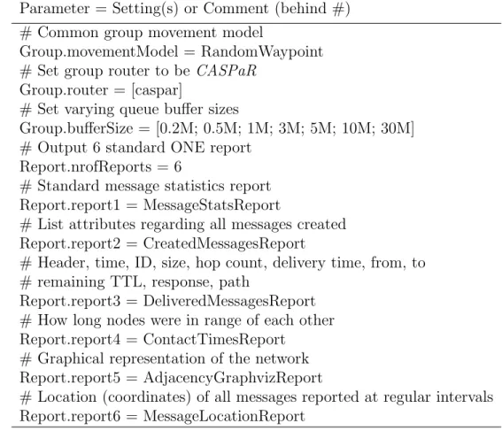
Congestion is caused by overuse of bandwidth within the network. Depending on the topology of the network, congestion can be a localized phenomenon or wide-spread. If congestion is localized then possibly the most effective means of bypassing it is to go around (avoid) it. If it is more widespread then there is no choice but to wait for it to subside; packet priorities being equal. Because DTNs do not behave as a continually-connected network, a typical approach to congestion control, Transmission Control Protocol (TCP) for example, does not work [17]. Congestion control must be designed into the routing protocol and avoided. The authors of [17] put forth a DTN congestion control taxonomy to classify congestion control techniques. Figure 1.3 shows a re-creation of the diagram that describes the taxonomy.

The taxonomy is divided into 8 main groups. The first, congestion detection, can be segregated into 3 categories: network congestion where the nodes try to de-tect congestion based on current throughput versus maximum throughput, buffer availability where nodes attempt to detect network congestion based on avail-able space in neighboring buffers and drop rate where nodes base congestion on packet drops. Another group is the control type and is partitioned into 2 categories: proactive congestion control which aims to prevent congestion from occurring and reactive congestion control which to reacts to reduce congestion once detected. The routing group indicates whether the congestion control mechanism is routing

(17)

Taxonomy Control Type Congestion Detection Open or Closed Loop Evaluation Platform Routing Contact Application Deployability Network Capacity Buffer Avail-ability Drop Rate Closed-loop Open-loop Proactive Reactive Hybrid Scheduled Predicted Opportu-nistic Dependent Indepen-dent Low Medium High

FIGURE 1.3. DTN Congestion Control Taxonomy: As first proposed in [17], this figure

shows the proposed DTN congestion taxonomy which we use to help classifyCASPaR’s

congestion control mechanism.

protocol dependent or independent and the contact group describes how contact between nodes in the network come in contact: in a scheduled fashion, a predictable fashion or completely randomly (opportunistically). The last group, deployability, describes how realistically deployable a congestion mechanism is.

1.4 Applications

The list of potential applications for a high-bandwidth capable, efficient and reli-able DTN routing protocol continues to grow and the networking boundaries be-tween them is blurring. Some DTN applications where CASPaR would be effective are described here.

1.4.1 Vehicular Network

Consider a vehicular network [18] that allows vehicles, traffic sensors, traffic control centers, gas stations, restaurants and all else travel, traffic and automobile related to communicate with each other on one network. How might these vastly different entities communicate? The travel stops such as gas stations, restaurants and hotels are all capable of TCP/IP base communication. But, the automobiles and traffic sensors form a network in which end-to-end connectivity isn’t guaranteed, a DTN. In the not so distant future, autonomous vehicles will have to communicate with

(18)

each other and with traffic sensors to efficiently and safely navigate. Cars might also communicate with gas and service stations and negotiate fueling or servicing options or appointments. Traffic sensors will route cars to less congested roadways, time lights to increase traffic throughput and ultimately ease traffic congestion and make traveling more safe. The cost effective nature of wireless communication makes it an obvious choice for vehicular networks. An elegant, efficient and simple networking solution is to create a mesh network from the sensors and vehicles themselves so that each and every one is responsible for relaying packets.

1.4.2 Interplanetary Network

Whether it be human or robotic, we are launching more things into space now than ever before. One commonality is that each of these spacecraft will have to communicate with home. As we travel further from Earth, a far-reaching space or interplanetary communication network (a deep-space network, DSN) will be needed (and already exists in some form [19]) to facilitate and route packets between home and these spacecraft potentially separated by millions of miles.

An example of the populating of our near-Earth space environment is the com-ing CubeSat revolution. David Pierce, senior program executive for suborbital research at NASA states that, ”CubeSats are part of a growing technology that’s transforming space exploration” [20]. A CubeSat is a small satellite approximately 10 centimeters cubed for a 1U (unit) sized model. They can be built in 2U, 3U, or 6U sizes as well. They weigh approximately 3 pounds per unit. Many are typically launched at once usually as axillary payloads making them launch-cost-effective. The number of small, sometimes tiny, space satellites are on the rise. These devices often can be designed and built for far less than their large heavy counterparts. Maybe more importantly, they can be launched for fractions of the cost.

(19)

Because technology has allowed for the miniaturization and greater efficiency of integrated circuits that perform all types of tasks, it is now feasible to build very small, relatively low-power communication devices that can be spread across vast regions of space building an interplanetary network to complement the existing DSN. This network is absolutely necessary if communication in and around our solar system is to be realized. Ultimately, localized interplanetary space travel hinges upon reliable communication.

1.4.3 Mesh Networking Solutions

General mesh networking solutions are being in explored in novel ways. An idea now coming to fruition is Google’s Project Loon [21]. Loon, aims to provide those in developing regions of the world internet access by flying LTE payloads (mini-cell towers) right above the tropopause at an altitude of 20 kilometers. Many of these balloons will be launched over a large area and provide mesh network coverage for anyone with an LTE enabled device in that region. Google Loon balloons currently achieve 100 days at float and have communication ranges on the order of 400 kilometers when several balloons are meshed in a single network. Float time and broadcast range are improving and as they do, LTE communication cost drops; possibly to the point that it will be cost effective to deploy communication balloon mesh networks in developed areas of the world; maybe here in the U.S. in congested areas where cell towers aren’t cost-effective or even feasible to construct.

This is a specific example of a broader push towards wireless, mobile, mesh communication allowing complete high-bandwidth connectivity between devices that may or may not always be connected. Routing techniques must be able to accommodate the potential for parts of the network to be delay and disruption tolerant and to bridge the highly mobile, mobile and non-mobile portions.

(20)

1.5 Motivation

Currently, there is not aone size fits all approach to MANET and DTN networking in general but maybe it is time to start working on it. Wireless communication and sensor devices perform all sorts of jobs but as wireless and sensor technology decrease in cost, their numbers will increase causing individual DTN islands to grow in numbers. As these islands begin to overlap they will merge. This process will repeat and as it does the DTN footprint will grow and its bandwidth requirements will expand. The clear delineation between MANETs, DTNs and even the internet will blur as devices once considered separate join the global network (globnet). This growth may continue until it reaches off-planet and the inter-planetary network one day joins the globnet. It is clear that there is a need for a common, efficient, robust routing protocol that can link these networks and account for specific DTN characteristics such as contact information, mobility pattern and network resources (storage space, transmission rate, and battery life).

1.6 Research Goals and Requirements

The development of a multi-purpose, one-copy DTN protocol that addresses con-gestion avoidance, shortest path routing and is capable of operating efficiently in a high-load network is the motivation behind the Congestion Avoidance Short-est Path Routing protocol (CASPaR). The algorithm is defined by the following developmental guidelines:

1. Do not duplicate packets.

2. Route deliverable packets, move undeliverable packets ’closer’ to their desti-nations and hold onto packets when prudent to do so.

3. Integrate congestion avoidance and bottleneck minimization into the design.

(21)

1. Learn direct routes to destinations when possible. 2. Avoid congestion.

3. Dynamically correct routes as the network topology changes.

4. Minimize latency and maximize delivery by moving packets over those newly discovered routes.

To do this, CASPaR must negotiate node queue differentials between

neigh-bors similar to back-pressure algorithms and map shortest paths without explic-itly discovering them. Here we present preliminary results showing that CASPaR

accomplishes these goals.

1.6.1 Derived Requirements

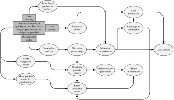
Figure 1.4 shows a flow diagram that presents the overall goal and constraints of CASPaR. It is a tool used to help derive the requirements of CASPaR whose overall goal is to deliver all packets as quickly as possible, for as long as possible

and as cheaply as possible under the restrictions of low memory, low power and

periodic disconnected nodes; typical restraints placed on a DTN.

Following the flow of the diagram shows, for example, that to deliver packets quickly,CASPaRmust move them closer to or directly to their destinations at each update interval but avoid congested routes when doing so. To avoid congestion, packets must be distributed evenly across the network topology and to accomplish this, probable routes must be known and queues must be balanced. Probable routes must be known in order to move packets closer to their destinations as well and to accomplish both of these objectives, queue and route information must be shared between nodes.

Because DTNs are defined by their disconnected paths, packets must be stored in the network until a route becomes available. Therefore, packets must be dropped

(22)

Conserve power Less broadcasts Distribute packets evenly Avoid congested routes Store fewer packets in buffers Less copies Move packets closer to destination Do not drop packets Minimize visited nodes Learn probable routes Share information Balance node queue sizes Less hops to destination Deliver all packets as

quickly as possible, for as long as possible and as

cheaply as possible. Low memory Low power Disconnected nodes Maximize queue usage

FIGURE 1.4. Goals and Requirements Chart: Lays out the overall goal and constraints ofCASPaR and the objectives and requirements that are derived from that overall goal. only as a absolute last resort which dictates efficient queue usage. Again, this re-quires an even distribution of packets across the network but also the minimization of node visits which means that fewer packet copies should be made and fewer vis-ited nodes enroute to a destination. This also requires that probable routes be discovered.

DTNs often have low-power restrictions and therefore energy conservation is a must. Power consumption is driven by the number of transmissions so by minimiz-ing broadcasts, power will be conserved. To do this, 2 thminimiz-ings must be constrained: 1) the number of hops a packet must make to get to its destination and 2) the number of duplicate packet copies must be minimized. Both of these restraints require that probable routes to destination nodes are learned .

Lastly, DTNs often have low-memory restrictions which means that few packets can be stored in each node’s queue and forces efficient queue management. This means that the number of nodes a packet traverses must be minimized which requires that there are fewer hops to the destination node and fewer copies of

(23)

packets. But to deliver packets quickly under these constraints, probable routes to destination nodes must be discovered.

This diagram identifies the requirements of an efficient DTN routing protocol design. An efficient protocol must share information between neighbors, makes few packet copies, if any, learn probable routes to destinations so that packets can be distributed over the network to avoid congestion and minimize routing hops.

1.7 Research Methodology Overview

The research methodology of theCASPaRstudy, whose goal is to develop a single-copy DTN routing protocol whose predicted routes avoid network congestion and form direct routes to destinations, is described in this section. First, existing DTN routing protocols were studied to better understand the DTN problem and to

de-termine which of the existing protocols should be used to compare with CASPaR

(the comparison protocols are referred to collectively ascomparison protocol). Once the DTN problem and existing solutions were better understood, a preliminary

version of the CASPaR algorithm was developed, tested (by simulation) and the

results compared withcomparison protocol results (using the same simulation pa-rameters). As problems and glaring inefficiencies with theCASPaR algorithm were discovered, they were studied, fixed and the algorithm was modified, tested and the results compared again. This refinement process included discussions amongst committee members and a few times involved tweeking the basic analytical model that theCASPaR algorithm is based upon. The entire process of testing, compar-ing and refincompar-ing was repeated over several iterations until the final version of the

CASPaR algorithm was created.

Once afinal CASPaR algorithm was developed, ’official’ protocol testing began. Testing involved a very specific network simulation where the only changes made between runs were the routing protocol, the random number generator seed and

(24)

the size of node buffers. The key comparison results were chosen to be delivery probability (messagesdelivered/messagessent), average message latency (the av-erage amount of time it takes all packets to be delivered), and hop count (the average number of nodes a message encounters before being delivered to its desti-nation). Special analysis attention was paid to the latency results which required simulation data reports accounting for all transmitted messages including their full paths from source to destination, their start times and their latencies.

To more completely gauge the high-performance behaviour ofCASPaR, anideal

single-copy routing protocol was required for comparison. A routing protocol that

knew the single shortest path between all source and destination nodes for all

queued messages at time t, one that could minimize hop count and latency while maximizing delivery probability was needed. TheShortest Path routing algorithm was developed to fill this need. To gauge low-performance behaviour, abasic single-copy routing protocol was required. The existing Direct Delivery routing protocol fit this requirement well. Remember that Direct Delivery is the routing protocol whose algorithm is one of self-delivery. That is, the only way a message is delivered is if the source and destination come within broadcast range or each other. To-gether, these two protocols provide the extreme case simulation comparison results. The other protocols that are simulated and compared in this study are:

1. Epidemic (EPI): Due to its potentially high overhead [8].

2. Prophet with Estimation (PRO): Due to its probabilistic routing [9].

3. MaxProp (MP): Due to it documented high-performance [11].

4. Backpressure LaB (LaB): To compare withCASPaR’s backpressure-like mech-anism [13] [14] [15].

(25)

5. Spray and Wait (SaW): Due to its high performance [12].

1.8 Thesis Outline

The rest of this thesis is organized as follows:

1. Chapter II describes theCASPaRalgorithm by detailing the analytical model it is based upon, providing the algorithm, describes an important variant and provides an example.

2. Chapter III describes the simulation, the simulation methodology, the specific simulator used including its input, execution style and report mechanisms. 3. Chapter IV provides the simulation results for delivery probability, latency,

overhead, and hop count. Some results and explanation of network load bal-ancing is also provided as well as a more detailed investigation into message or packet latency.

4. Chapter V has some concluding remarks and discusses some ideas into pos-sible future study regardingCASPaR.

(26)

Chapter

2 CASPaR

CASPaR is a one-copy routing protocol that attempts to route packets over the

shortest, least congested paths. CASPaR consists of two interdependent

mecha-nisms: 1) direct routing and 2) congestion avoidance. The algorithm is designed to route packets over connected paths and employs a routing-protocol-dependent, proactive congestion-avoidance mechanism [17] that uses an open loop congestion control scheme based on buffer availability and historical connectivity knowledge. This allows for alternate route discovery avoiding congestion buildup. Ultimately, congestion avoidance takes precedence over routing forcing a direct-delivery-like mode of operation during heavy traffic. Except for their 1-hop neighbors, nodes have no knowledge of other nodes in the network.

2.1 Principle of Operation

All nodes maintain an estimated cost (C_nc(t)) to deliver packets to each destination nodec. This cost attempts to track the least congested and shortest paths to each destinationc based on historical knowledge of connectivity to the destination and the waiting times of packets to c in node n’s queue. The process by which Cc

n(t) is calculated begins with the broadcast of a Request For Costs (RFC). All nodes participate in the RFC transaction process when one of three things occurs: 1) a packet has just been received from a neighbor, 2) a packet has just been created or 3) the RFC periodic timer expires. Neighboring nodes, upon receiving an RFC, respond with their destination cost table which contains a list of all destinations and the cost to send a packet to that destination. If node n’s estimate of delivery costs to c is the lowest amongst its neighbors, then n holds onto these packets

(27)

in its buffer until it either meets a neighbor with a better (lower) estimate or is connected to c (we use a preference factor of 0.9 to give a slight preference to nodenholding onto these packets). Priority transmission is given to those packets whose destination are neighboring nodes. The effect of periodic updates is a more accurate network congestion and connectivity model and since routes depend upon a neighbor’s total transmission costs, frequent updates produce a more applicable model (similar to distance vector routing in wired networks [1]). Nodes have no direct knowledge of the state of the network outside of its own neighborhood. But due to the propagation of costs, each node gains an approximate network-wide perspective allowing for effective packet routing.

2.2 Model

Path congestion and route connectivity are modeled by minimizing the delivery costs along some multi-hop path from source to destination and is characterized by two convoluted parameters: The first isProximity Measure:

Θc_n(t) = Q c n(t) Tc n(t) (2.1) Θc

n(t) is a value between 0 and 1 where 1 indicates nodesn and care connected and 0 means they were never connected.Tc

n,t is incremented at every time step and Qc_n,t is set equal to T_n,tc as long as nodes c and n remain connected forcing Θc_n(t) equal to 1. Once disconnected, Θc

n(t) begins decreasing linearly in time. Periodically bothQ and T are reset to some initial values that represent a default measure of connectivity. The second parameter is the Net Destination Queue Waiting Time:

W_nc(t) = N

X

i=0

(T −ac_n,i) (2.2)

where T is the current time and ac

n,i is the arrival time of packet i at node n destined for node c. The queue waiting times of packets are used as a proxy for

(28)

congestion as opposed to backpressure which uses queue size differentials. Hence, we model delivery costs as an exponentially increasing function of net waiting times of packets with an increasing discount factor based on connectivity probability. The estimated delivery costs toc via n are calculated as:

C_nc(t) = W_nc(t)˙(1−Θc_n(t)) +C_nc(t−1) (2.3)

CASPaR’s, estimated delivery cost is calculated while explicitly setting trans-mission costs between 1-hop neighbors to 0. This emphasizes routing along a con-nected path between source and destination when one exists, and routing to bal-ance congestion in the network when connected paths do not exist. Setting 1-hop transmission costs to 0 has the following effects: 1) If a connection from source n to destination c exists then the delivery cost will be 0 everywhere along that path regardless of path length sinking packets directly to destinationc(see line 24 from Alg. 1) and 2) If a connection from source n to destination c does not exist then packets to c will be spread over the network based on congestion, radiating outwards towards the destination. Eventually when one of these nodes becomes connected, a direct path tocis created and packets quickly flow down-gradient to their destinations.

In addition to Θc

n(t) being set to 1, the historical cost,Cnc(t−1), is reset to 0 when nodes n and c become connected at time t. From the definition of W earlier, the marginal increase in net waiting times at each time step are a function of queue size toc. Thus as can be seen from the expression above, lightly congested nodes along short paths to the destination are favored (the more recently a node is in contact with the destination and the smaller its queue size, the lower the transmission cost) and therefore the net effect of the algorithm is to reinforce delivery on short, less congested paths.

(29)

Proximity Measure andNet Destination Queue Waiting Time, parameterize not

only the shortest but least congested paths. The Proximity Measure attempts to

minimize the path length from source to destination whileNet Destination Queue Waiting Time pulls packets towards neighboring nodes with the smallest queues (similar to a backpressure mechanism [16]) minimizing routing across congested paths. This technique develops routes thatchase the destination, ultimately catch-ing and creatcatch-ing short paths from source to destination.

Packets are transmitted in a lowest-cost first, longest-queue-waiting-time second, priority order. More simply put, the oldest, cheapest packets are transmitted first. Also, a minimum node loop counter to force a Minimum Loop Size (MLS) is integrated into the CASPaR algorithm to avoid packets repeatedly traversing the same nodes. The MLS is defined to be the minimum number of consecutive unique nodes that must exist in a routing path before a packet is allowed to revisit a node. The MLS is set to 5 for all simulations presented here.

2.3 Algorithm

Request for Costs is executed both periodically and upon the receipt or creation of a packet. The range status, measure of proximity, net destination queue waiting time and total transmission costs are recalculated upon each call (see Alg. 1 and Table 2.1).

2.4 Multi-path Variant

Several variations of the CASPaR protocol were designed and tested during this

DTN study. Two that emerged as notable candidates are theCASPaRand

CASPaR-MP. The ’standard’ variant, defined by single path costing is designed based on costs to route packets to the neighbor that replies with the lowest relay cost based on single routes to destinations. It is referred to as single-path costing or the

(30)

TABLE 2.1. Algorithm Definitions Cc

n(t) The transmission cost for all packets destined for node cthat reside in node n’s queue at time t.

Wc

n(t) The net destination queue waiting time is the amount of time that all packets destined for node c have been resident in node n’s queue at time t. Θc

n(t) Proximity Measure that is analogous to the elapsed time since nodesn and cwere within k-hop radius of each other such that 0<Θc_n(t)≤1. When nodesn and care connected, Θc

n(t) = 1. If

nodesn and j have never been connected, Θn,j(t) is 0.

Rc

n,t The range status between node n and destination c at

time t. If node cresides in the k-hop neighborhood of noden at timet, the range status, (rc

n,t), is set to true. Otherwise it is set to false.

ac_n,i The arrival time of theith packet at node n destined for node c.

Tc

n,t A tick counter which is incremented upon each bid period.

It is reset to some default measure of connectivity periodically. Qc

n,t Counter incremented each time nodes n and c are not

neighbors. It is reset to some default measure of connectivity periodically.

τ The current time.

CASPaR-SP variant. Since it is the standard algorithm it is always referred to as

simply CASPaR.

A slight modification of CASPaR takes steps to distribute packets more widely over the network as an enhanced congestion avoidance technique and is referred to as the multi-path or simply CASPaR-MP. Instead of calculating costs based on a

single route from a relay node to a destination, CASPaR-MP takes into account

all possible routes to a destination during the cost determination process.

The multi-path designation may be somewhat of a misnomer. It does not mean that messages are split and sent across different routes towards their destination nor does it mean that a relay node will alternate between routes when sending messages to some set destination. It means only that route costs are calculated

(31)

Algorithm 1The CASPaR Algorithm

1: functionUpdate Range Status 2: for alldestinationsdo

3: ifdestinationcis within 1-hop of nodenthen

4: Rc

n,t= true

5: else

6: Rc

n,t= false

7: functionUpdate Measure of Proximity 8: for alldestinationsdo

9: Tc

n(t) =Tnc(t) + 1

10: ifRc

n,tthenQcn(t) =Tnc(t) .Periodically reset to default values

11: Θcn(t) = Qc_n(t)

Tc n(t)

12: functionUpdate Queue Waiting Time 13: for alldestinationsdo

14: Wnc(t) = PN

i=0(T −acn,i)

15: functionUpdate Delivery Cost 16: for alldestinationsdo 17: ifRcn,tthenCnc(t−1) = 0

18: Cc

n(t) =Wnc(t)˙(1−Θcn(t)) +Cnc(t−1)

19: functionRequest for Costs 20: Update Range Status () 21: Update Measure of Proximity () 22: Update Queue Waiting Time () 23: Update Delivery Cost ()

24: Cc

n(t) = 109C˙

c

n(t) .Calculate Self-Delivery Estimate

25: for allnodesjin 1-hop range of noden, for all destinationscdo

26: SelectCc

m= min(Cjc(t), Cnc(t)) and relayraccordingly

27: UpdateCc

n(t) =Cmc and either relay packet to nodejor do not transmit ifr=n

based upon all possible routes to each destination from some relay node instead of basing it on the single lowest cost route. It will, however, behave in such a manner as to allow for separate back-to-back messages to very likely be transmitted over different routes. This is demonstrated in Figure 2.1.

Take a network that consists of nodes n, j1, j2, and cand paths x, y and z for

example. Nodenwishes to deliver a packet to nodecand must select the node that reports the minimum cost to be the relay. Nodej1 is connected to node cthrough

two paths,x andy. Node j2 is connected to nodecthrough only one path, z. Out

of all paths, x, y and z, z is the least congested and therefore the single cheapest

route. However, because nodej1 can offer 2perceived independent paths, nodej1’s

presented cost may be less than node j2’s depending on the cost-combination of

the individual bids. In the case shown in Figure 2.1, xhas a cost of 3,y has a cost of 3 and z has a cost of 2. The cost presented to n byj1 to transmit a packet to

(32)

j

1

j

2

n

c

FIGURE 2.1. Multi-path Diagram: Shows the functionality of CASPaR-MP. Node j1

has 2 routes, x and y to destination node c both at cost 3. Node j2 has only one route

zat a cost of 2. In single-path routing, node nwould choosej2 to send packets through

since it has the single lowest cost route. However, in multi-path routing, node n could

choose j1 depending on the combined cost of its two parallel routes.

C_nc(t) = 1/ N

X

i=0

(1/pi) (2.4)

where pi is the ith path.

In the scenario presented here, the cost reported to node n by j1 is 3/2 which

is less then the cost presented by j2 which is 2 and therefore packets destined for

c would be transmitted through relay j1 at time t. Assuming this scenario, node

n would choose j1 to send packet-1 onto destination c. Lets assume that j1 sends

packet-1 through path x. Now lets say another packet, packet-2 is sent by node n to nodej1. Nodej1 re-processes a RFC and it is now likely, since packet-1 may still

reside in the buffer of the node only 1-hop away from node j1 along path x, that

path y will produce the lower cost and hence packet-2 will be sent through path

y towards its destination c. From this example, it can be seen how CASPaR-MP

can easily be conformed into a routing protocol capable of splitting packets and send them across varying routes.

(33)

5 3 4 0 0 0 2 3 j3 c T=1 j1 n j2 c j1 j2 j3 2.7 3 4 5 (a) Time T=1 6 4 5 1 0 1 3 4 j3 c T=2 j1 n j2 c j1 j2 j3 3.6 ‐ ‐ 6 (b) Time T=2 7 5 6 2 1 2 4 0 j3 c T=3 j1 n j2 c j1 j2 j3 4.5 ‐ ‐ ‐ (c) Time T=3 8 6 7 3 2 0 0 1 j3 c T=4 j1 n j2 c j1 j2 j3 5.4 ‐ 1 ‐ (d) Time T=4

FIGURE 2.2. CASPaR Example Diagram: ACASPaR example iterating through 4 time

periods and the transactions between a group of nodes in a small network.

It is shown in the results that CASPaR-MP does provide a slight advantage

overCASPaR. However, it was not chosen as the standard because of its analytical

complexity and minimal performance gains when compared toCASPaR.

2.5 Example

In the scenario presented in Figure 2.2, the weighted graph represents a small net-work. The vertices represent nodes:n, j1, j2, j3,andc. The weighted edges represent

the transmission cost between nodes (a weighted-edge of 0 represents neighboring nodes). In this scenario, noden is to deliver a packet to nodec. Each panel repre-sents a time-step and depicts a single RFC transaction. There are 4 panels starting atT = 1 and ending with the delivery of the packet at T = 4. Queue sizes aren’t explicitly considered in the transmission cost and the measure of proximity is cal-culated using integers for simplicity. The self-delivery costs are multiplied by 9/10 as the algorithm is defined. At the bottom left-hand corner of each panel is the

destination cost table showing all potential destination nodes and their associated costs.

At T = 1, node n broadcasts a RFC. Nodes j1, j2 and j3 respond with their destination cost tables and node n compares them against its self delivery cost. These values are shown in the representative destination cost table:c= 2.7,j1 = 3,

j2 = 4 and j3 = 5. Since self delivery cost is the minimum, node n holds onto the

(34)

Node n is unaware of the state of the network beyond its own neighborhood. After the RFC responses are received, node n learns its neighbors: j1, j2 and j3

and that they can deliver a packet to node c for 3, 4 and 5 respectively. Node n deduces that a direct route to node cdoesn’t exist since a minimum delivery cost of 0 wasn’t received. Noden selects itself as the relay since its delivery cost is the minimum.

At T = 2, node n again broadcasts a RFC but this time only nodej3 responds.

The other nodes have moved out of range. Since the self delivery cost, incremented

to 4 from time period T = 1 to T = 2, is still the minimum, node n again holds

onto the packet.

Node n has no neighbors at T = 3 and by default its cost is the minimum and

noden continues to hold the packet. Notice, that nodesj1 andcbecome neighbors

at this time. Unfortunately node n can not know this since it isn’t connected to nodej1.

Finally, at T = 4, node n is a neighbor of node j2 who responds with the

minimum delivery cost of 1. Node n transmits the packet to node j2 who will

transmit the packet to node j1; provided that nodes j1 and j2 are still neighbors

once j2 is ready to re-transmit.

The network is dynamic and can change quickly. The receipt of the packet from node n causes node j2 to initiate its own RFC transaction that might reveal a

route change. Other nodes potentially in the path might update their destination cost tables due to received and generated packets or because the update timer expired. A transmission cost of 0 reveals an end-to-end connection from current source to destination and can trigger an avalanche of packet transmissions towards the destination.

(35)

Chapter

3 Simulation

3.1 Purpose and Methodology

The purpose of the simulations was to compare the performance of CASPaR, its

multi-path variant and 7 additional routing protocols as a function of buffer size. A realistic yet simple simulation was required that placed all protocols on equal footing. A relatively high data throughput was desired to stress the nodes in the network but the transmission rate was set to resemble typical LTE transfer rates of about 5 Mbps as measured from an actual LTE phone on AT&T’s network in Baton Rouge, Louisiana. Systematic effects of the simulation were considered to ensure that A) there were no special case simulation runs for any of the tested protocols and B) if large variations existed in simulation results for a particular routing protocol and simulation scenario, they were known and their deviations accounted for. Therefore, the simulation had to be run multiple times but with different random number generator seeds to generate different results.

This called for a simple simulation scenario with few modifiable parameters

as this thesis is an introductory study of CASPaR. The only parameters that

were modified were the routing protocol, the buffer size and the random number generator seed for the node movement engine. The results had to include delivery performance in terms of probability, latency and overhead. The results also had to include all routes taken for all messages delivered including latencies and number of hops. These results were needed to perform more in-depth analysis on latencies as a function of routing.

Two candidate network simulators, NS-2 and ONE, were reviewed. The ONE simulator was chosen for its Java programming interface, its realtime simulation

(36)

GUI, because it is specifically geared towards DTNs and because it already has many of the standard DTN routing protocols contained within the installation.

3.2 The ONE Simulator

The Opportunistic Network Environment simulator (ONE) version 1.4.1 [22] was used for all simulations performed during this study. ONE is a graphical network simulator specifically designed for simulating DTNs. It comes with standard rout-ing algorithms includrout-ing Direct Delivery, Epidemic, PRoPHET, Spray And Wait

and MaxProp all of which were simulated along with CASPaR. ONE provides a java programming interface complete with all classes required to design, develop, incorporate and simulate the behavior and performance of new routing algorithms. It is also capable of collecting and reporting network summary data that can be easily collated and analyzed.

With it, nodes can be created, placed within a blank or elaborate map and translated according to many different movement models. Some of the common ones are: random waypoint, map-based random waypoint and map-based routed movement models. There are also movement models designed specifically for dif-ferent vehicles like cars and buses, and for difdif-ferent times of the day like work day hours and evening trends. While movement is being orchestrated, broadcast communication is simulated between nodes within range of each other. Each node has its own broadcasting time-slice and the selection rotation is randomized.

All simulations were run using the java runtime engine (jre) version 1.8.0 40 and all coding was written, compiled and run using the Eclipse Standard Software Development EnvironmentVersion: Kepler Service Release 1Build id:20130919−

(37)

3.2.1 Input

Various input parameters are loaded at execution time in the form of aparameter initialization file. The parameter initialization file used for CASPaR simulations is provided in the appendix. These parameters define key simulation attributes. These key attributes include definitions for: overall scenario settings, broadcast settings, nodes and node movement, routing, event and message generation and summary reporting. The overall scenario settings include: the overall map size, the update interval, the number of different node groups, the random number generator seed to use for the movement model and the length of time that the simulation is to be run. The broadcast settings include: the radio interface used by a group of nodes, and the transmission range and speed of that radio interface. The node settings include: the number of nodes in a group, the movement model used by that group of nodes as well as the group movement speed and wait time. The routing parameters include: the type of router used by a group of nodes, its buffer size, and type and its message or packet time-to-live (TTL). The event and message generation settings include: the different event generation groups, the message generation rate for each group, the message size and the range of message source and destination addresses. The summary reporting parameters detail which reports are generated and various specific settings that a report might require. For example, the message location report which tracks the location of all messages requires the reporting granularity parameter set in seconds. This indicates the interval at which the location of messages is recorded.

The ONE simulator allows for various groups of nodes, radio interface and move-ment models to be defined as well as various groups of event generators. These groups can be mixed and matched to create a very versatile simulation. Many parameters can also be defined as a range. Movement speed, for example, can be

(38)

defined to be between 0.5 and 1.5 meters per second. When these degrees of free-dom are combined, it allows for quite complex simulations. The default scenario, the Helsinki model for example, consists of various groups of nodes, some pedes-trians, cars, and trams all traveling at appropriate speeds and moving according to map-based movement models where pedestrians walk on sidewalks, cars drive on roads and trams travel the same routes over and over on rail throughout the map of Helsinki. Pedestrians and cars have a different broadcast range and rate than do the trams. This scenario presents a more realistic scenario and much more complicated ones can be constructed.

The simulation environment can also be quite simple as well. The simulation

model used for the CASPaR study is one such example. The movement model is

a random way point where nodes randomly pick a point to move to then move to that point at some defined speed or range of speeds. Once they arrive, they wait there for some randomly determined amount of time then pick a new point and the process repeats until the simulation ends.

The parameter initialization file allows for multiple settings to be specified for most of the parameters by simply adding to a comma-delimited list bounded by brackets. See Table 3.1. When run in batch mode, ONE is capable of executing multiple iterations one after another. Upon each new simulation run, parameters in comma-delimited list format are iterated through one after the other and used as the input parameters for that run. If only a single setting is present for a parameter, the setting will be repeated for each execution.

3.2.2 Execution

Simulations can be run in either graphical or batch mode. A graphic mode simula-tion can be run from within the development environment and provides a graphical runtime view of the network grid and the movement of nodes within the grid. It

(39)

provides views to each node’s queue and packet routing information. It is a good tool to learn the behavior of the routing algorithm being designed and tested. It does slow simulations down, consuming valuable CPU cycles, so for multiple simulations it is best to run in batch mode.

FIGURE 3.1. ONE Graphical Interface: The ONE graphical interface includes simulation control, a node movement view and packet routing information.

Figure 3.1 shows the ONE simulation GUI. Towards the top are the simulation control buttons: play, pause, speedup and step-through are all available. The net-work grid can also be resized. The upper-left shows the simulation elapsed time and the number of simulation cycles per second currently being executed. At the bottom left is the event log and event log control. The event log displays critical events such as message creation, delivery and drop as well as when connections are made or lost. The types of events that are displayed is controlled using the check boxes in the event log control. Along the right side of the GUI is the list

(40)

of nodes present in the simulation. The coordinate location, number of messages in queue and routing information for all messages to and from any node can be displayed by clicking on any one of the node numbers. This is an invaluable tool when designing, implementing and testing a new routing algorithm.

Batch mode allows multiple simulations to be run from a single command line

execution by using the multiple simulation option -N where N is the number of

simulation runs to be performed. As previously stated, batch mode also allows parameter settings to vary between runs but this requires proper construction of theparameter initialization file. Notice in Table 3.1 theGroup.bufferSizeparameter has 7 different buffer size settings comma-delimited within brackets. When run with N = 7, 7CASPaR simulations would be run, each with a different buffer size; first

0.2 MB, then 0.5 MB, then 1.0 MB and so on through 30 MB. If N was set to 8,

the settings just wrap around to the beginning of the list, and therefore the 0.2 MB buffer size setting would be used again. All multiple parameter settings function in this manner. For every run, the next setting in the list is used until the end of the list is reached at which point it starts at the beginning of the list. This allows building complex batch jobs to run many time-consuming simulations as opposed to running them individually.

3.2.3 Reporting

The ONE simulator offers many reporting tools that are engaged by simply adding the report name to the parameter initialization file. Detailed here are the couple reports used to produce the results discussed in this paper.

The Message Statistics Report, as shown in Table 3.2 contains a summary re-port of all nodes for an entire simulation. It contains the standard results used to produce the following plots as a function of queue buffer size: Delivery Prob-ability, Overhead Ratio, Hop Count and Packet Latency. The key statistics used

(41)

TABLE 3.1. Example Parameter Initialization File: An excerpt from a parameter ini-tialization file showing specifically how to vary parameters between multiple run batch mode execution. Anything behind a # is a comment.

Parameter = Setting(s) or Comment (behind #) # Common group movement model

Group.movementModel = RandomWaypoint

# Set group router to be CASPaR

Group.router = [caspar]

# Set varying queue buffer sizes

Group.bufferSize = [0.2M; 0.5M; 1M; 3M; 5M; 10M; 30M] # Output 6 standard ONE report

Report.nrofReports = 6

# Standard message statistics report Report.report1 = MessageStatsReport

# List attributes regarding all messages created Report.report2 = CreatedMessagesReport

# Header, time, ID, size, hop count, delivery time, from, to # remaining TTL, response, path

Report.report3 = DeliveredMessagesReport # How long nodes were in range of each other Report.report4 = ContactTimesReport

# Graphical representation of the network Report.report5 = AdjacencyGraphvizReport

# Location (coordinates) of all messages reported at regular intervals Report.report6 = MessageLocationReport

in this report are the number of dropped messages, the number of delivered mes-sages, the delivery probability, the latencies, the overhead ratio and the hop count measurements.

The Message Delivery Report details when and how long each message takes to get from the source to destination as well as the path or route the message tra-versed. Table 3.3 is an excerpt of one message delivery report. The report contains a listing (in rows) for all delivered messages. In the report header, the Time is the time that the message was sent, the MsgID is tagged message identification num-ber, the Size denotes the size of the message, Hops indicates the number of hops from source to destination,Lat refers to the latency, the time needed for a message

(42)

TABLE 3.2. Example Message Statistics Report: An example of a message statistics report produced from the ONE simulation.

Stat Value simtime: 3600.0260 created: 3600 started: 129442 relayed: 129441 aborted: 0 dropped: 0 removed: 129441 delivered: 3264 deliveryprob: 0.9067 responseprob: 0.0000 overheadratio: 38.6572 latencyavg: 214.9006 latencymed: 76.2370 hopcountavg: 35.2007 hopcountmed: 17 buffertimeavg: 6.3682 buffertimemed: 0.1480 rttavg: N aN rttmed: N aN

to get from source to destination, Src and Dst are the source and destination of the message respectively, TTL is the remaining TTL of the packet at the time of delivery, Rsp indicates if a response was received and Path details the entire path of the message including source and destination.

TABLE 3.3. Example Message Delivery Report: An example of a message delivery report produced from the ONE simulation.

Time MsgID Size Hops Lat Src Dst TTL Rsp Path

1.036 M1 100000 1 0.036 p75 p6 n/a N p75 p6

18.019 M18 100000 1 0.019 p62 p67 n/a N p62 p67

45.066 M45 100000 2 0.066 p32 p45 n/a N p32 p88 p45

(43)

3.3 Shortest Path Routing

Shortest Path is an semi-omnipotent router based upon Dijkstra’s shortest path algorithm. It was created as the standard by which all simulated protocols are measured. For this protocol, the shortest path between every node and destination is calculated at each update interval and messages are routed accordingly. The shortest path is likely to change between update intervals which is why the shortest path is re-calculated each update period. The simulation results of Shortest Path

represent the upper-bound on the delivery performance.

Shortest Path is not the optimum solution. It is limited to knowing the optimum state of the network at timetand not the optimum solution at all timest+nwhere n= [1,2,3, ...]. The term semi-omnipotent in this case means, knowing all shortest paths in the network at this moment in timet.

3.4 Parameters

All thesis results were obtained using the same random way point simulation sce-nario, referred to as the Random Scenario. Each protocol was tested using the same set of buffer sizes and run 17 times with different random number generator (RNG) seeds to negate systematic simulation affects. Table 3.4 lists the simulation settings.

3,600 messages are created during the 1 hour simulation. Source and destination nodes are chosen randomly therefore each node is just as likely as any other to source or sink messages. The message time-to-live (TTL) is 300 minutes, explicitly set to be greater then the total simulation time so that TTL doesn’t play a role in dropped messages. Messages are queued (but not necessarily transmitted) in FIFO order and only dropped due to queue overflow or protocol-based metrics.

The network map is 1 square kilometer, the radio broadcast range for all nodes is 100 meters, the message (packet) size is static at 100 kilobytes and there are 100

(44)

nodes that participate in the network simulation. The nodes can move randomly over the map at between 0.5 and 1.5 meters per second (walking speed) and once they’ve reached their target they will hold for anywhere between 0 and 1 second before continuing on to their next randomly chosen destination.

The nine different routing protocols that were tested and whose results are re-ported are:

• Direct Delivery (DD) [23]: Self-delivery.

• Epidemic (EPI) [8]: Packet flooding.

• Prophet with Estimation (PRO) [9]: Probabilistic routing.

• MaxProp (MP) [11]: Transmission and drop prioritization.

• Backpressure LaB (LaB): Combination between Backpressure and the future position of the message in the neighbor’s queue.

• Spray and Wait (SaW) [12]: Bounded multi-copy routing.

• Shortest Path (SP): Omnipotent shortest path.

• CASPaR (CASPaR): Single-copy, single-path.

(45)

TABLE 3.4. Simulation parameters as used by the Random Scenario simulations

Parameter Description Value

World size 1km x 1km

Node count 100

Simulation Update Interval 0.037 seconds

Network packet rate 1 per second

Run time 3,600 seconds

Transmit speed 10 Mbps

Transmit range 100 meters

Buffer-sizes tested .2, .5, 1, 3, 5, 10 and 30 MB

Send queue FIFO queue

Node speed 0.5 - 1.5 meters per second

Node wait time 0.0 - 1.0 seconds

Message TTL 5 hours

Message period 1 second

Message size 100 KB

Node movement RandomWayPoint

Movement warmup period 100 seconds

Map Open map

Protocols tested Direct Delivery, Epidemic, PRoPHET,

MaxProp, Spray and Wait, LaB

Shortest Path, CASPaR and CASPaR-MP

Queue Type FIFO

Number of reports 6

Reports Message Statistics, Created Messages

Delivered Messages, Contact Times Adjacency Graph, Message Location

Message location granularity 60

MaxProp timescale 10

PRoPHET seconds in time unit 10

Spray and Wait number of copies 6

Spray and Wait mode binary mode

CASPaR mode single path OR multi-path

CASPaR: Congestion Avoidance Shortest Path Routing for Delay Tolerant Networks

Louisiana State University

LSU Digital Commons

CASPaR: Congestion Avoidance Shortest Path

Routing for Delay Tolerant Networks

Michael F. Stewart

Acknowledgments

Table of Contents

List of Tables

List of Figures

Abstract

Chapter

1

Introduction

Chapter

2

CASPaR

j

j

n

c

Chapter

3

Simulation