Machine learning methods for
detecting structure in metabolic
flow networks
Maxwell Jay Conway
Selwyn College
This thesis is submitted for the degree of Doctor of Philosophy.
Declaration
This dissertation is the result of my own work and includes nothing which is the outcome of work done in collaboration except as declared in the Preface and specified in the text. It is not substantially the same as any that I have submitted, or am concurrently submitting, for a degree or diploma or other qualification at the University of Cambridge or any other University or similar institution except as declared in the Preface and specified in the text. I further state that no substantial part of my dissertation has already been submitted, or is being concurrently submitted, for any such degree, diploma or other qualification at the University of Cambridge or any other University or similar institution except as declared in the Preface and specified in the text. This dissertation does not exceed the prescribed limit of 60 000 words.
Maxwell Jay Conway August, 2018
Abstract
Machine learning methods for detecting structure in
metabolic flow networks
Maxwell Jay Conway
Metabolic flow networks are large scale, mechanistic biological models with good predic-tive power. However, even when they provide good predictions, interpreting the meaning of their structure can be very difficult, especially for large networks which model entire or-ganisms. This is an underaddressed problem in general, and the analytic techniques that exist currently are difficult to combine with experimental data. The central hypothesis of this thesis is that statistical analysis of large datasets of simulated metabolic fluxes is an effective way to gain insight into the structure of metabolic networks. These datasets can be either simulated or experimental, allowing insight on real world data while retaining the large sample sizes only easily possible via simulation. This work demonstrates that this approach can yield results in detecting structure in both a population of solutions and in the network itself.
This work begins with a taxonomy of sampling methods over metabolic networks, before introducing three case studies, of different sampling strategies. Two of these case studies represent, to my knowledge, the largest datasets of their kind, at around half a million points each. This required the creation of custom software to achieve this in a reasonable time frame, and is necessary due to the high dimensionality of the sample space.
Next, a number of techniques are described which operate on smaller datasets. These techniques, focused on pairwise comparison, show what can be achieved with these smaller datasets, and how in these cases, visualisation techniques are applicable which do not have simple analogues with larger datasets.
In the next chapter, Similarity Network Fusion is used for the first time to cluster organisms across several levels of biological organisation, resulting in the detection of discrete, quantised biological states in the underlying datasets. This quantisation effect was maintained across both real biological data and Monte-Carlo simulated data, with
related underlying biological correlates, implying that this behaviour stems from the net-work structure itself, rather than from the genetic or regulatory mechanisms that would normally be assumed.
Finally, Hierarchical Block Matrices are used as a model of multi-level network struc-ture, by clustering reactions using a variety of distance metrics: first standard network distance measures, then by Local Network Learning, a novel approach of measuring con-nection strength via the gain in predictive power of each node on its neighbourhood. The clusters uncovered using this approach are validated against pre-existing subsystem labels and found to outperform alternative techniques.
Overall this thesis represents a significant new approach to metabolic network structure detection, as both a theoretical framework and as technological tools, which can readily be expanded to cover other classes of multilayer network, an under explored datatype across a wide variety of contexts. In addition to the new techniques for metabolic network structure detection introduced, this research has proved fruitful both in its use in applied biological research and in terms of the software developed, which is experiencing substantial usage.
Acknowledgements
First of all, thanks to Pietro Li´o, for his exemplary support, guidance and encouragement. I’d also like to thank the rest of the group, particularly Claudio Angione, for numerous ideas and excellent advice.
Thanks to my various collaborators throughout the PhD, not only for the data they provided but also for the huge amount I learnt from them, and thanks to the EPSRC— without their financial support this would not have been possible.
And finally, my deepest thanks to my family and friends, both new and old, for their invaluable help and support, both intellectual and emotional.
Contents
1 Introduction 9 1.1 Overview . . . 9 1.2 Papers . . . 12 2 Background 14 2.1 Introduction . . . 142.2 A simplified view on how cells work . . . 14
2.3 How to model living cells . . . 16
2.3.1 Approaches to modelling cells: which black box to choose . . . 17
2.3.2 Approaches to modelling cells: the metabolome is relatively tractable 18 2.4 Metabolic modelling . . . 18
2.5 Overview of existing metabolic network analysis techniques . . . 21
2.6 Optimisation . . . 23
2.6.1 Linear programming . . . 24
2.6.2 Evolutionary optimisation . . . 24
2.7 Networks . . . 25
2.7.1 Metabolic networks . . . 25
2.7.2 Similarity and distance networks . . . 26
2.7.3 Network representations . . . 26
2.8 Review of state of the art in genome-scale metabolic modelling techniques . 26 2.8.1 Constructing, obtaining and improving metabolic models . . . 26
2.8.2 Unbiased methods . . . 27
2.8.3 Biased methods . . . 29
2.8.3.1 Flux Balance Analysis (FBA) . . . 30
2.8.3.2 Regulatory methods . . . 32
2.8.4 Genetic perturbation . . . 35
2.8.5 How this work fits in . . . 36
3 Characterising state spaces of flow networks: sampling metabolic
mod-els 38
3.1 Introduction . . . 38
3.1.1 Overview . . . 39
3.2 Inducing variation to create sample spaces . . . 40
3.2.1 Modifying the environment . . . 41
3.2.2 Modifying network structure by removing reactions . . . 41
3.2.3 Modifying network structure by adding reactions . . . 42
3.2.4 Modifying objective values . . . 43
3.2.5 Modifying reaction rates directly using gene expression data . . . . 44
3.2.6 Taking advantage of slack in model . . . 45
3.3 Sources for prior distributions over sample spaces . . . 47
3.3.1 Gene expression sampling . . . 48
3.3.2 Evolutionary sampling . . . 49
3.3.3 Environment modification . . . 49
3.4 Case studies . . . 50
3.4.1 Implementation: Fbar . . . 51
3.4.2 Case study 0: Placeholder sampling approach . . . 52
3.4.3 Case study 1: Batch based proportional adjustment . . . 52
3.4.4 Case study 2: Evolutionary sampling with environment variation . . 54
3.5 Conclusion . . . 56
4 Small sample approaches 57 4.1 Introduction . . . 57
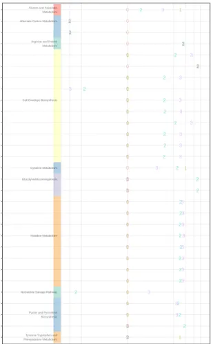
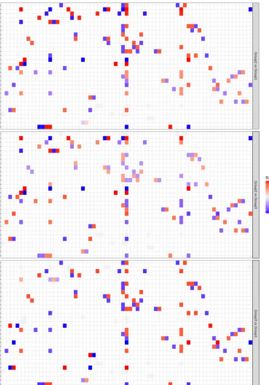
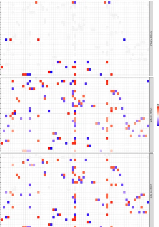
4.2 Comparison across 11 samples from 4 gene expression conditions . . . 58
4.2.1 Preprocessing and methods . . . 59
4.2.2 Postprocessing and results . . . 60
4.2.3 Conclusion . . . 64
4.3 Pairwise statistical and visual comparison via evolutionary optimisation: Metabex . . . 64
4.3.1 Conclusion . . . 69
4.4 A platform for examining small numbers of models: FBAonline . . . 69
4.4.1 Conclusion . . . 71
4.5 Conclusion . . . 71
5 Network interpretation by Similarity Network Fusion 73 5.1 Introduction . . . 73
5.2 Overall approach . . . 74
5.3.1 Motivation . . . 76
5.3.2 Definition of W . . . 76
5.3.3 Definition of P0 . . . 77
5.3.4 Definition of S . . . 77
5.3.5 Core operation . . . 78
5.4 Weighted Similarity Network Fusion tool . . . 78
5.4.1 Further changes to weighted SNF tool . . . 79
5.5 Application . . . 80
5.6 Similarity Network Fusion on simulated data . . . 81
5.7 Validation . . . 82
5.8 Conclusion . . . 83
6 Hierarchical Block Matrices and Local Network Learning 86 6.1 Introduction . . . 86
6.2 Testing on synthetic data . . . 86
6.3 Network structure measures . . . 87
6.4 Local Network Learning based similarity measures . . . 91
6.4.1 Predictivity gain . . . 91
6.4.2 Predictivity gain applied to metabolic networks . . . 92
6.4.3 Calculating predictivity . . . 93
6.4.4 Choice of supervised learning algorithm . . . 94
6.4.5 Applying network local predictive power based similarity measures . 95 6.4.6 Reducing computational load by enhancing graph sparsity . . . 95
6.5 Validation . . . 98
6.6 Conclusion . . . 99
7 Future work 102 7.1 Network of networks vs structure of solution spaces . . . 102
7.2 Precomputing datasets for FBAonline . . . 102
7.3 Other flow network data . . . 103
8 Conclusion 104
CHAPTER
1
Introduction
1.1
Overview
Metabolic networks are one of the most successful approaches to modelling how living cells work. They are capable of making verifiably correct predictions [1] from mecha-nistic simulations of whole cell biochemistry, and are used extensively in academic and industrial biotechnology [2]. However, with hundreds [3–5] of these models available, each with hundreds or thousands of reactions, approaches to generating real understanding are lagging behind black box predictive power.
This work introduces and demonstrates a number of statistical and machine learning approaches to network structure detection. The central hypothesis is that inference from large datasets of feasible metabolic flow configurations is an effective way to derive infor-mation about the structure of a metabolic network. Specifically, the simulated datasets used here are of optimal networks, which have been optimised by linear programming under some set of conditions, based on small perturbations around a high biomass value. This is slower than uniform sampling, but I argue in Chapter 3 that it is more biologi-cally justifiable, and it is more directly comparable with techniques used on experimental data. As well as being relatively under explored in the context of metabolic flow net-works, these techniques have the distinct advantage that they can be applied to both real data and Monte Carlo simulations even where the properties of the input data are poorly understood or characterised.
Chapter 2,Background, describes biological background, such as the shape, properties, and reasonable assumptions about metabolic networks, and why these properties make them amenable to computational simulation and analysis. It also describes technological background: network representations, relevant mathematical theory, and related works.
Chapter 3, Characterising state spaces of flow networks: sampling metabolic models, describes a taxonomy of methods for Monte Carlo sampling on metabolic networks,
or-ganised by frameworks for methods of modifying models and sources for distributions to bias the modifications selected. It then finishes with a selection of example case studies of sampling strategies, which are used as demonstration data in Chapter 5 and Chapter 6.
Chapter 4, Small sample approaches, describes three different approaches to creation and interpretation of small sample sizes of metabolic networks in concrete biological set-tings. A central thread of this chapter is that all three methods attempt different ways of understanding metabolic networks visually, and while these have their strengths, they also demonstrate the need for statistical techniques that can detect network structures. This forms something of a counterpoint to the methods in chapters 5 and 6, which deal with much larger sample sizes.
Chapter 5, Network interpretation by Similarity Network Fusion, describes the ap-plication of the Similarity Network Fusion [6] technique to metabolic datasets. This is applied to both a real world gene expression dataset and to simulated data, in order to show patterns in the samples in both datasets. The results are clustered, resulting in the types of phenotype groupings which would typically be attributed to genetic variation. However, the results are similar across both experimental and simulated datasets, and have related underlying causes, implying that these clusters in fact stem from network structure itself.
Chapter 6,Hierarchical Block Matrices and Local Network Learningdescribes a project to detect and uncover latent structure in flow networks by combining biased Monte Carlo sampling with a local network approach to unsupervised detection of important network links. This is applied to detect network structure in both real and simulated datasets, and is validated by comparison with pre-existing manual subsystem labels. The results are shown to be significantly better predictors of subsystem labelling than would be expected by chance, and to outperform off the shelf clustering techniques.
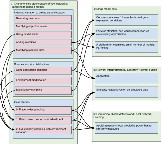
Figure 1.1 shows some of the links between chapters in terms of data or techniques. This emphasises the overall structure of the thesis: Chapter 3 focusses on techniques and examples of data generation, while chapters 4, 5 and 6 introduce techniques and examples of data interpretation.
3: Characterising state spaces of flow networks: sampling metabolic models
Inducing variation to create sample spaces
Sources for prior distributions Removing reactions
Adding reactions Modifying objective values
Modifying reaction rates Using model slack
Gene expression sampling
Case studies
0: Placeholder sampling
1: Batch based proportional adjustment
2: Evolutionary sampling with environment variation
4: Small model sets
Comparison across 11 samples from 4 gene expression conditions
Pairwise statistical and visual comparison via evolutionary optimisation
A platform for examining small number of models: FBAonline
5: Network interpretation by Similarity Network Fusion Application
Similarity Network Fusion on simulated data
6: Hierarchical Block Matrices and Local Network Learning
Applying network local predictive power based similarity measures
Environment modification
Evolutionary sampling
Figure 1.1: Diagram of links between chapters. Arrows represent links of either data usage or technique usage: where the data and techniques introduced in Chapter 3 are used in the other chapters. Green boxes represent chapters, blue boxes represent sections, red boxes represent subsections and so on. Sections on theory or implementation which are not shared between chapters are omitted for brevity.
1.2
Papers
The following is a list of publications that I have been involved with throughout my PhD. Of these, [7, 8] are particularly relevant to Chapter 2, [9–11] are particularly relevant to Chapter 4, and Chapter 5 is based on work in [12]. All work covered in this thesis is wholly my own, along with the associated portions of these papers, though other parts of the papers were done in collaboration.
• [13]: Bioinformatics challenges and potentialities in studying extreme environments. Claudio Angione, Pietro Li, Sandra Pucciarelli, Basarbatu Can, Maxwell Conway, Marina Lotti, Habib Bokhari, Alessio Mancini, Ugur Sezerman, Andrea Telatin. International Meeting on Computational Intelligence Methods for Bioinformatics and Biostatistics, pages 205–219, 2015. In this paper I advised on the metabolic networking content.
• [12]: Multiplex methods provide effective integration of multi-omic data in genome-scale models. Claudio Angione, Maxwell Conway, Pietro Li´o. BMC Bioinformat-ics, 2016. In this paper I contributed all of the work on Similarity Network Fu-sion, while the simulation component was done in collaboration. Since then I have reimplemented the simulation component myself for convenience, as is described in Chapter 5.
• [10]: Iterative Multi Level Calibration of Metabolic Networks. Maxwell Conway, Claudio Angione, Pietro Li´o. Current Bioinformatics, 2016. In this I created the multi-objective optimization procedure (though starting from an existing code base described in [14]), and did all other work: creating the visualisation framework described and all scratch.
• [7]: Seeing the wood for the trees: a forest of methods for optimization and omic-network integration in metabolic modelling. Supreeta Vijayakumar, Maxwell Con-way, Pietro Li´o, Claudio Angione. Briefings in bioinformatics, 2017. To this review I contributed the tutorial section, and some of the body text, and two of the three figures.
• [9]: Transcriptome and proteome analysis ofSalmonella entericaserovar Typhimurium systemic infection of wild type and immune-deficient mice. Olusegun Oshota, Maxwell Conway, Maria Fookes, Fernanda Schreiber, Roy R Chaudhuri, Lu Yu, Fiona JE Morgan, Simon Clare, Jyoti Choudhuri, Nicholas R Thomson and others. PloS one, 2017. In this paper I contributed all work involving metabolic modelling: 5 of the written sections and figures 4 to 6.
• [8]: Optimization of Multi-Omic Genome-Scale Models: Methodologies, Hands-on Tutorial, and Perspectives. Supreeta Vijayakumar, Maxwell Conway, Pietro Li´o, Claudio Angione. Metabolic Network Reconstruction and Modeling, pages 389– 408, 2018. I contributed the perspective in section 4 to this background piece.
• [11]: CiliateGEM: an open-project and a tool for predictions of ciliate metabolic variations and experimental condition design. Alessio Mancini, Filmon Eyassu, Maxwell Conway, Annalisa Occhipinti, Pietro Li`o, Claudio Angione, Sandra Puc-ciarelli. BMC bioinformatics, 2018. In this project I created tools that were used for sections 3 and 5 of the CiliateGEM pipeline in figure 1.
• [15]: STAble: a novel approach to de novo assembly of RNA-seq data and its application in a metabolic model network based metatranscriptomic workflow. Igor Saggese, Elisa Bona, Maxwell Conway, Francesco Favero, Marco Ladetto, Pietro Li`o, Giovanni Manzini and Flavio Mignone. BMC bioinformatics, 2018. For this paper I provided advice and discussion.
CHAPTER
2
Background
2.1
Introduction
This chapter describes biological background, such as the shape, properties, and reason-able assumptions about metabolic networks, and why they are amenreason-able to computational simulation and analysis. It also describes technological background: network representa-tions, relevant mathematical theory and related work.
This chapter begins with biological background covering the motivation and justifi-cation for the techniques used here (sections 2.2, 2.3 and 2.4), before moving on to an overview of comparable techniques in section 2.5. Technological background is discussed in sections 2.6 and 2.7, before concluding with a detailed review of related techniques in 2.8. Background which is exclusively relevant to particular analytic techniques is left to the appropriate chapters. Particular emphasis is placed on areas that are relevant to simulation based, rather than analytic, techniques for network structure detection, since this is the focus of this thesis.
2.2
A simplified view on how cells work
Humans, like most animals, solve many of our problems by mechanics. If we do not like something, we move away from it. If we are hungry, we go to a place that has food, find it, and eat it. However, this gives us something of a skewed view on what life is: for instance, children often do not immediately think of plants as alive.
Life is primarily about chemistry. Living organisms are cells (occasionally more or less cooperating colonies of more than one cell, like us), and a cell is a bag of chemicals. These chemicals pull outside chemicals into the bag, convert them into useful materials, and expel unwanted by-products. They then use the acquired building materials to construct more biomass (the materials that make them up) until they get large enough to split, and
continue growing.
Most of the molecules in a cell are broadly described as metabolites. These are all the small molecules which form the feedstocks, intermediaries and by-products, for growth within the cell. A good way of thinking of this is that this includes almost everything that one would learn about in high school chemistry, rather than in biology. For instance, water, oxygen, hydrogen ions, salts, sugars, and alcohols.
The heavy lifting of these chemical processes is done by proteins. These are built from long chains of amino acids, connected end to end, which fold and coil into useful shapes that allow them to perform useful functions. Of particular interest are enzymes, which are proteins which facilitate chemical reactions between metabolites, and transporter proteins, which form tunnels and pumps to move metabolites into and out of the cell. Proteins often perform these functions in surprisingly mechanical manners: enzymes are typically shaped to bind loosely to their substrates in such a way as they are forced together to react before being released, whilst active transporters typically operate via a ratcheting principal.
Proteins are large molecules composed from a small set of unique amino acids (20 in humans), chained together. The information on what sequences of amino acids make up each protein is stored in DNA. Once again, this is a chain of subunits from a small alphabet, though in this case there are only four symbols, known as nucleotides, which are interpreted with groups of three encoding each protein.
The process of constructing proteins from the DNA template is known as ‘gene ex-pression’. (Potentially confusingly, ‘gene expression’ also refers to the quantitative rate of this process.) It works as follows:
1. A protein complex called RNA polymerase attaches itself to the DNA strand, split-ting open the double helix to read one side.
2. The RNA polymerase protein moves along the strand. At each DNA nucleotide, it attaches a complementary nucleotide of mRNA (mRNA is much like DNA, but more reactive and less stable). It then binds the mRNA nucleotide to the previous mRNA nucleotide.
3. When the RNA polymerase finishes its work, the result is an mRNA negative of the gene that is required.
4. A large protein called a ribosome attaches to the mRNA negative to read it into a protein.
5. Once again, the ribosome moves along the mRNA, this time attaching matching tRNA bases. The tRNA is present in groups of three bases, with each group attached
to one amino acid. The ribosome moves along the mRNA, using the tRNA to attach the correct chain of amino acids together, to create the required protein.
6. The amino acids in the chain curl up to bind to each other to form the correct three dimensional shape.
This process appears quite simple when described in such general terms, however it in-volves a very large amount of detail and incidental complexity, as described in section 2.3.
2.3
How to model living cells
The mechanisms of gene expression described in the previous section are conceptually fairly simple. In many ways, the manufacturing of proteins is simpler than the manufac-turing of many consumer goods—although proteins are far more complex and intricate end results, the process of instantiating them from their ‘blueprint’ has quite uniform steps.
However, if we want to model how living things behave, we need to know how their metabolism acts, since this is the primary way that most of them interact with the outside world. We also need to know this in a quantitative manner, and this is where we run into serious complexity.
Because the individual mechanisms are generally well understood and relatively simple, it is possible to construct differential equations that accurately describe each part of the process in isolation. However, once these equations are connected together the system explodes in complexity due to the many, many feedback loops. These feedback loops make characterising the system very difficult because it is difficult to experiment on parts in isolation, and because attempts to isolate subsystems in vitro inevitably alter the environment. Furthermore, for in vivo experiments, measurement and perturbation are difficult. Cells are small, so normally measurements can only be taken on large numbers simultaneously, meaning that only an aggregate result can be found. Because the result is aggregated across many different cells, any effect must be large in order to be detectable, and so the perturbation must be large to generate a detectable result, and to overcome the cell’s attempts to counteract it.
Furthermore, because life is evolved rather than designed, much of the regulation and control occurs via what could be described as inelegant methods, which represent local fitness maxima. As an example, if there is too much of a metaboliteX, the amount could be reduced by any combination of a vast number of more or less direct methods. For instance, the amount of the enzyme that creates X could be reduced by interfering at any point in its transcription process, or by blocking it from acting, or the opposite could be done to an enzyme that breaks it down, or alternatively any of these actions could
be conducted on an indirectly connected enzyme which acts on a different metabolite to create a knock on effect on the production or degradation ofX, or its uptake or removal. Or, indeed, nothing could be done at all, and the cell could perform some other action to just cope with the excess of X. In a designed system, one would hope that there would be a deliberate choice of the most simple and direct method to achieve an end. However in an evolved system the pattern seems to be that the first mutation that helps with a problem is selected for, and any resulting side effects are dealt with later.
2.3.1
Approaches to modelling cells: which black box to choose
When faced with a complicated system, it is common to start by choosing some compo-nents to model mechanistically, and some to model as a black box, finding the easiest model that fits the data under the relevant circumstances.
Taking this approach, systems biology has tended towards an overall view that consid-ers the cell as a set of conceptual layconsid-ers, termed ‘omes’. This naming is from the genome, the set of all genes in the cell.
Unlike the other ’omes, the genome is generally static, and when changes do happen these are normally random mutations during copying, rather than any kind of directed change, or short term feedback. This means that most or all of the information about how an organism works must be included in the genome. Fortunately, the stability, structural uniformity and random mutations of the genome also make it easy to study. If you observe a property of an organism and later sequence its genome, then you know that the genome you find was the same as the genome at the time of observation, and that it is extremely unlikely that a genetic feature is a result of some other property of the organism. In the past, particularly prior to the human genome project, there was a hope that if we sequenced enough genomes and compared them with enough phenotypes (the external properties of an organism), then we would be able to infer the genotype-phenotype relationship black box, and that this would give us a predictive model of how life worked.
It should come as no surprise to those from a computer science background that this did not work. The genotype-phenotype relationship is stochastic and stateful. It has as an input tens of thousands of genes (ignoring the vast number of variations that they can take), and has as an output another incredibly complex relationship: a mapping from a vast number of poorly defined aspects of the environment to an equally vast set of potential phenotypic effects. Attempting to understand this kind of relationship without looking at the underlying mechanisms is therefore intractable in the general case.
2.3.2
Approaches to modelling cells: the metabolome is
rela-tively tractable
In the previous section, the problems associated with trying to model the genotype pheno-type relationship as a black box were discussed. Of course, the alternative to this approach is to take a more reductionist and mechanistic approach, starting our understanding with simple, well understood subsystems and slowly expanding our understanding outwards.
The metabolome has a number of properties that make it a good area to begin:
• Small molecules are generally completely identical to each other. This contrasts with larger structures like proteins where small variations cannot be individually tracked, since this would lead to a combinatorial explosion.
• The molecules in the metabolome are generally present in large enough quantities that quantisation effects can be ignored.
• Because the molecules of the metabolism are small, they diffuse quickly and their orientation can be ignored.
• The interactions between many groups of small molecules have already been well studied by organic chemists in vitro, so that there is already theory with good predictive power, at least until enzymes get involved.
• As discussed previously, chemical exchange is one of the main ways that small organisms interact with the outside world, so metabolic models accurately capture much of their phenotype.
The gold standard in describing metabolic subsystems are systems of partial differ-ential equations. Unfortunately, it is complex and difficult to accurately measure the reaction rate coefficients required, and these models explode in complexity as more and more elements are added and subsystems are joined. This means that if we want to model the complete metabolism of even a very simple organism, we need to use models with less parameters.
2.4
Metabolic modelling
Rate coefficients to chemical reactions can be difficult to measure, especially when they are enzyme mediated, since many, many factors can influence the abundance and activity of enzymes. However, the stoichiometry (the participants and their ratios) of chemical reactions is fixed, since this is determined by conservation of matter and of charge.
Lists have been constructed that detail the stoichiometry of biological reactions, with coverage of most of the reactions that occur in most organisms. Reactions that are
Respiration Photosynthesis Water CO2 Oxygen Glucose ATP ADP CO2 Water
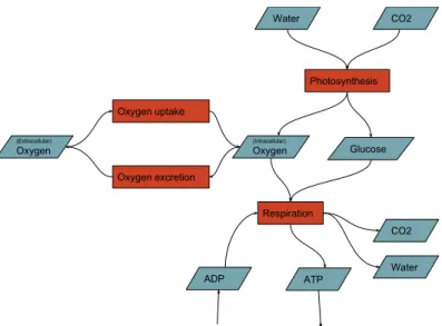
Figure 2.1: A simplified sketch of a metabolic network. In this sketch, we can see that if glucose is conserved and in steady state, the rates of photosynthesis and respiration must be equal. Glucose, water, and CO2 are examples of metabolites, whilst photosynthesis and respiration are examples of reactions.
missing tend to be unique to particular groups and only used under specific circumstances, such as breaking down unusual foodstuffs or providing protection from toxins, so a large proportion of the reactions occurring in common organisms in benign environments can be covered.
These sets of reactions can be considered as flow networks. As discussed in sec-tion 2.7.3, there are a few different ways in which these can be represented, but the simplest model (aside from those that discard information) is to consider the relationship between reactions and metabolites as a bipartite graph: both reactions and metabolites are nodes, with reaction nodes only having edges to metabolite nodes, and vice versa. Edges are directed to represent either consumption or production of a metabolite, and numbered with the stoichiometry of the link. Reactions have a rate, and the rate at which they produce a particular product is their own intrinsic rate, multiplied by the stoichiometry of the link to the product.
From this position, we can start adding assumptions. The first of these is a steady state assumption. This says that there is no net surplus or deficit of any metabolite, so the total rate of production of a metabolite is equal to the total rate of consumption.
This is equivalent to Kirchoff’s current law in electronics [16], and means that the rates of the reactions producing the metabolite are tied to the rates of the reactions consuming it. Obviously to allow uptake and excretion this assumption must be relaxed in some areas, which is normally achieved by one sided placeholder reactions. We also add some constraints on rates of reactions. Typically these are quite liberal except for the uptake and excretion placeholders, which we generally assume to be the among the limiting points in the system.
At this stage, we have what is known as a flux space. This is a space with a number of dimensions equal to the number of reactions, and a polytope within this space enclosing the feasible region—the set of reaction rate assignments that are consistent with the assumptions, consistent with the constraints, and consistent with all of the other reaction rates. Figure 2.1 shows a simple example of a metabolic network, showing the different node types and resultant constraints.
If we stop here and directly explore the still under-constrained flux space, we have what are known as unbiased methods. These are decomposition methods that project the full set of dimensions of the flux space down onto a somewhat smaller set of dimensions that cover only the feasible flux space. Unbiased analytic methods such as elementary flux modes are the state of the art in analytic understanding of flow networks, but they have a number of disadvantages in the analysis of large metabolic networks:
1. in typical applications, whilst the dimension reductions are significant, they are still not enough to enable human interpretation,
2. the assumption of a uniform and unbiased flux space is not necessarily reasonable,
3. these approaches are difficult to apply to multi-level models or to real data, and
4. despite being analytic rather than simulation based, they are highly computationally demanding.
Of course, there are various approaches to address each of the weaknesses of unbiased analytic methods, but this thesis eschews these methods in favour of statistical and ma-chine learning post-processing of flux data sets, since this affords increased flexibility and the ability to apply techniques uniformly to a variety of types of models, simulations, and real world data.
If we attempt to find individual solutions within the flux space that are particularly biologically likely, or important, then we have biased methods.
Biased and unbiased methods are both described in more detail in section 2.5 on the next page.
There are many biased methods, but the prototypical method, on which most others are based, is Flux Balance Analysis (FBA). This adds one extra assumption to the model
previously outlined: that evolution has already optimised the organism to grow as fast as possible. To use this assumption we add another placeholder reaction to the existing uptake and excretion nodes—a sink for biomass. This reaction simulates the sequestra-tion of materials that is required for growth, and is generally a reacsequestra-tion with a very large number of input reactants. Unusually the biomass reaction typically has fractional stoichiometries, since we can find the ratios of materials required for growth by simply analysing the constituents of a whole cell.
Once we have a biomass equation, we have a direction for optimisation. We find the assignment of fluxes that will achieve the highest biomass production. This is normally achieved by Linear Programming, which is a fast, specialised optimisation method that is applicable to this type of problem. In small models, this optimisation process can find a single flux assignment, finding a single value for all reactions, but in larger models this is not always the case, as discussed in section 3.2.6 on page 45.
2.5
Overview of existing metabolic network analysis
techniques
The most common and in many ways best model for a system of chemical reactions is a system of differential equations. The problem is that building such a system requires knowledge of rate coefficients for every reaction, which are difficult to measure, especially for enzyme catalysed reactions in vivo. This makes that approach intractable for full organism models.
Therefore, techniques to analyse large metabolic models must get by with just stoi-chiometry and various other constraints on reaction rates, such as constant bounds. These methods can be divided into two groups [17]: biased methods make the assumption that evolution has evolved to optimise for certain properties of the reaction system, such as maximising biomass production, and simulate this maximisation to find rates; unbiased methods make no such assumptions.
Unbiased methods are typically analytic decompositions of the flux space such as Elementary Flux Modes [18], although some uniform Monte-Carlo approaches exist, while biased methods are typically variants on Flux Balance Analysis.
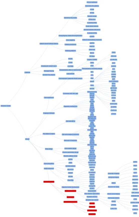
Section 2.8 describes in detail the field of available techniques for both biased and unbiased optimisation, in conjunction with figure 2.2, which organises the taxonomy of different techniques visually.
However, the central dichotomy of purpose, as well as methodology, between biased and unbiased methods is extremely important to understanding the purpose of this the-sis: biased methods are primarily predictive, since they focus on specific model states, while unbiased methods aim to produce descriptive results. On a high level, these two
ap-Figure 2.2: A tree diagram providing an overview of the field of metabolic modelling. Red nodes represent techniques and software introduced in this thesis: Biased structure detection techniques by combining Monte-Carlo simulations, visualisations and unsupervised clustering. A zoomable version is available online atwww.cl.cam.ac.uk/~mjc233/metabolic_modelling.
proaches exist because whole cell metabolic models are very complex systems. Unbiased approaches such as Elementary Flux Modes are effective as descriptive tools, in that they capture uniformly all possible states of the model, but this is not necessarily possible with large models, nor is it always desirable, since some model states are more important than others. By contrast, biased models capture individual states of the system, one by one. This makes them very good at specific predictive tasks, but because they only capture one state at a time, they provide little descriptive power—they are very good at answering questions like ‘what happens if this reaction stops?’, but they are very poor at answering questions like ‘which pathway is this reaction in?’. One purpose of this thesis is to com-bine these two approaches by using large scale biased simulations to describe metabolic networks. The aim is to provide descriptive tools over multiple states of models, but with the advantages of biased tools, by focusing on flux distributions that are optimal under some conditions.
2.6
Optimisation
Mathematical optimisation refers to searching the domain of a function in order to find an argument or set of arguments such that the result of the function, or some property of the result of the function, is as large or as small as possible. The most common objective is simply to minimise the function result, where this result is often a measure of error or cost.
In metabolic modelling it is common to see two different types of optimisation which serve quite different purposes, but are easily confused, so it is worth distinguishing between them.
The first is optimising the network fluxes to maximise the biomass objective function. Because of the assumptions made about the metabolic network, this optimisation problem can be expressed as a set of linear inequalities in what is termed canonical form. This structure can be exploited by techniques such as the Simplex algorithm to find the global optimum very quickly. We can term this part the inner optimisation problem. It is concerned with choosing flux assignments to simulate a plausible biological result.
Secondly, it is common to also use an outer optimisation algorithm, which alters the parameters to the inner optimisation problem. This outer optimisation is typically concerned with the constraints to reaction rates (rather than reaction rates themselves), and at each iteration will test a set of reaction constraints by using the inner optimisation algorithm to find the fluxes implied by those constraints.
Whilst the inner algorithm can typically be evaluated very quickly (typically less than 1 s in the applications described here), the outer optimisation algorithm cannot easily exploit any structure of the function that it is optimising over (which involves evaluation
of the inner algorithm), and so must run the inner algorithm at every iteration, meaning that a much more generic optimisation algorithm must be used, with much longer running times.
A discussion of linear programming (the typical technique for solving the inner opti-misation problem), and evolutionary optiopti-misation (a common technique for solving outer optimisation problems) follows.
2.6.1
Linear programming
Linear programming (‘programming’ is here used in the pre-computational sense of de-signing a schedule) is a technique for optimising a certain restricted class of systems which include metabolic networks. By virtue of their restricted problem class, linear program-ming solvers can be made much, much faster than more general optimisation techniques like gradient descent, whilst also providing much stronger guarantees about the result optimality.
Linear programming addresses optimisation problems that can be expressed in the form ‘maximisecT·x, subject to linear constraintsx≥0 andA·x≥b’. These constraints
can be interpreted as a polyhedron in which any valid solution must fall. The solution is the point on the polyhedron that is furthest in the objective direction. The simplex algorithm exploits the fact that a global optimum must be found at one of the vertices of this polyhedron, and works around the vertices to find this solution. Where an edge or face of the polyhedron is perpendicular to the objective direction, an infinite number of globally optimal solutions may exist, but there will still be one at each vertex adjacent to this edge or face.
Linear programming is used in a wide variety of contexts, but economically important resource allocation problems are often particularly amenable to this approach. Fortu-nately, this creates a relatively lucrative market that has produced a number of fast and highly optimised solvers, both open source and commercial. The three solvers used most in this research are Gurobi, one of the fastest commercial solvers, with an academic li-cence, GNU Linear Programming Toolkit (GLPK) [19–21], a relatively fast and reliable open source solver, and Embedded Conic Solver (ECOS) [22, 23] for some testing and simple problems, since it is self-contained and easy to install.
2.6.2
Evolutionary optimisation
Evolutionary optimisation is a description for a wide range of optimisation algorithms that generally maintain a population of independent solutions, generate new solutions from the old solutions via a random mutation process, and discard low quality solutions in favour of higher quality ones. Many evolutionary optimisation algorithms take inspiration from
features of biological evolution, such as generating new solutions by a pairwise sexual recombination process.
Evolutionary optimisation algorithms do not generally keep track of population level aggregate statistics, do not generally require a concept of landscape gradient, and are afforded some robustness against local minima by keeping a wide population. These properties make them suitable for use in optimising systems that are difficult to char-acterise. Furthermore, their wide population of solutions means that they can be used as part of a process of characterising a complex fitness landscape, since they can give information on a variety of local minima.
Both of these properties make them suitable for use on the outer optimisation step of metabolic networks, since they are able to address these complex problems whilst also providing information on the shape of the entire solution space.
2.7
Networks
The word ‘network’ generally denotes a set of nodes and edges, where each edge connects two nodes (or sometimes a node to itself), and each node has zero or more edges connected to it. This description is applicable to a vast number of areas, with different explicit assumptions about network structure and the properties of nodes and edges, and often implicit assumptions about what different features mean.
2.7.1
Metabolic networks
This thesis primarily discusses chemical reaction networks, which are a type of flow net-work. Comparing to other flow networks might lead us to jump to a description where metabolites (chemicals) are nodes, and reactions are edges, a bit like a logistics network where we could think about metabolites as stores of matter with conversions between them. Alternatively, we might think about reactions as nodes, with metabolites being edges between them, much like in a traffic network where junctions allow flow to change directions.
However, metabolites can take part in multiple reactions, and reactions can have more than one substrate and one product, so in fact both must be considered as nodes, edges between them purely indicating stoichiometric coefficients. A missing edge is a coefficient of 0. Since reactions can only be connected to metabolites and vice versa, this graph is bipartite. The alternative to this would be to use the hypergraph generalisation, where edges can connect multiple nodes.
2.7.2
Similarity and distance networks
When discussing machine learning it is also important to touch on the concepts of similar-ity and distance networks, which are networks where edge weights represent the similarsimilar-ity or dissimilarity between nodes, under some measure. When discussing the representation of these quantities as networks, as opposed to distance or similarity matrices, it is also necessary to consider the implications of unconnected nodes. When nodes are not con-nected many algorithms take this to be equivalent to an edge weight of 0. This means that for machine learning applications, similarity networks are often more convenient than distance networks, since it makes sense for unrelated nodes to have a similarity of 0, whereas in a distance network setting, unrelated nodes would have an undefined or infinite distance.
2.7.3
Network representations
There are a number of different ways to represent networks in a tabular or matrix format, with different relative merits in terms of their convenience for certain computational operations, and the mental model that they encourage. For metabolic modelling, there are a few representations that are particularly useful. Adjacency matrices are matrices where both rows and columns represent nodes, whilst non-zero entries in the matrix represent edges. These are convenient because, if we use the bipartite nature of the graph to only list metabolite nodes in rows, and reaction nodes in columns, then the adjacency matrix of the network is the stoichiometric matrix of the reaction system. If we take a sparse representation of the adjacency matrix, we get an edge list, which in the context of metabolic modelling is a list of metabolite, reaction pairs. Finally, a convenient format is a reaction list, which can be interpreted as a kind of adjacency list, where for each reaction node we have the name and stoichiometry of each metabolite that is involved.
Representing networks in a manner that is amenable to machine learning is an open area of research, with a number of approaches introduced recently [24–26]. Chapter 6 discusses an approach to breaking down a large network learning problem into a series of smaller ones that are more similar to traditional tabular datasets.
2.8
Review of state of the art in genome-scale metabolic
modelling techniques
2.8.1
Constructing, obtaining and improving metabolic models
Whole genome metabolic models are available online in repositories such as the Kyoto Encyclopaedia of Gene and Genomes, also known as KEGG [4], the Biochemical Genetic
and Genomic knowledge-base (aka BiGG) [27], the BioCyc collection of pathway/genome databases [28] MetaNetX [29] and ModelSeed[30], among many others. In addition, many of the newest are available first only as supplementary information to papers. The prepa-ration of a genome-scale metabolic model involves the reconstruction of all metabolic reactions taking place in the organism, annotated and extended with supplementary in-formation on the genes, metabolites and pathways. Reconstructions vary significantly in quality, both in terms of their format and ease of parsing and the completeness of their underlying information, and as such, manual curation and gap filling is sometimes required [31]. One technique for this is to reconcile predictions from models with in-vivo
findings in order to identify gaps in our knowledge of metabolism [32].
Inconsistencies often exist between models and experimental data. This can be false positives or false negatives for boolean model properties, or poor correlations in numeric model properties. Algorithms exist to support the identification and correction of some classes of inconsistencies, such as Grow Match [33], SMILEY [34] and Optimal Metabolic Network Identification (OMNI) [35]. Finding inconsistencies can not only lead to im-provements in model quality, but can sometimes also guide basic biological research [36]. GapFind and GapFill are examples of optimisation procedures which identify problematic metabolites which are known to exist in a cell but for which no known reaction either produces or consumes them, and propose mechanisms to restore pathway connectivity for these metabolites [37]. FastGapFill [38] is an extension of FASTCORE which incor-porates flux and stoichiometric consistency to guide the gap filling process. Metabolic Reconstruction via Functional Genomics (MIRAGE) [39] conducts gap-filling by inte-grating with functional genomics data to estimate the probability of including any given reaction from a universal database of putative gap-filling reactions in the reconstructed network. This enables selection of the set of reactions, the addition of which is most likely to result in a fully functional model when flux analysis is done again. Many models also integrate signalling and regulatory pathways with metabolic networks in order to add information regarding underlying mechanisms.
2.8.2
Unbiased methods
As described earlier, unbiased methods search the whole solution space of a metabolic model to find sets of statistically analysable states without requiring the definition of a specific objective function. These techniques are therefore similar in principle to other unsupervised techniques in machine learning, although they aim to explore the statistical properties of a network model, rather than the tabular datasets that are pervasive in general purpose unsupervised methods.
Network-based pathway analysis is a large family of unbiased methods which assess the main properties of biochemical pathways [40]. Gene Association Network-based
Path-way Analysis (GANPA) improves upon this process by adding gene weights to determine gene non-equivalence within pathways [41]. A similar approach to this was recently pro-posed to compare pathway significance by constructing weighted gene-gene interaction networks in healthy and cancerous tissue samples [42], which could then be used to ex-pand pathways for each set of samples and to compare their topologies. Network-based pathways enrichment analysis is another technique to identify a greater number of gene interactions. An example of this is NetPEA, which utilizes a protein-protein interaction network in combination with a random walk to include information from high throughput networks and known pathways [43]. The NetGSA framework is another example of where condition-specific data has been used in combination with network estimation in order to improve the detection of differential activity in pathways [44].
A variety of different methods can be used for network-based pathway analysis, to calculate the set of routes through the reaction network and the corresponding matrices which represent their stoichiometry. Elementary flux modes (EFMs) describe the minimal, non-decomposable set of pathways that operate within a steady state system. These are found by the repeated removal of single reactions until a valid steady state flux distribution cannot be calculated [18]. This process tends to yield a vast number of common functional motifs - this is one of the problems common to unbiased methods which the techniques in this thesis avoid. However, other techniques exist to attempt to address these large numbers of motifs. Agglomeration of Common Motifs (ACoM) can be used to cluster these motifs, with overlap between classes allowed [45]. Another approach is to determine a single elementary flux mode by solving an optimisation problem using EFMevolver [46]; this can draw attention to significant elementary flux modes. Finally, K-shortest EFMs enumerates elementary flux modes in order of their number of reactions, since the shortest pathways are often of most biological interest due to their high flux and experimental tractability [47].
A further approach to network based pathway analysis is Generating Flux Modes [48]. The set of Generating Flux Modes is the smallest set required to define the geometry of the flux space using a null-space algorithm. The number of GFMs is often extremely large, but it is possible to identify specific subsets with more reasonable computational re-quirements [49]. In addition, there exist methods for dimensional reduction of flux cones, such as minimal metabolic behaviours [50] and minimal generators [51]. One method is to search for the shortest path between a given pair of end nodes [52], but the assumptions made in this approach are often criticised as overly simplistic, since they ignore actual re-action stoichiometry, throwing away a large amount of information [53]. Thermodynamic constraints can be used to add additional network information, such as in tEFMA [54], which removes thermodynamically infeasible EFMS using network-embedded thermody-namic (NET) analysis [55]. This use of thermodythermody-namic information can be extended to
identify for physiologically significant EFMS, since the largest thermodynamically consis-tent sets (LTCSs) of EFMs often represent condition-specific metabolic capabilities [56].
Extreme pathways are an important subset of EFMs [40]. They consist of the minimal, independent set of reactions required to exist as a functional unit, and are characterised by a set of convex basis vectors which represent the edges of the steady-state solution space [57]. Most of the methods described here are intended to reduce dimensionality, however EFMs increase dimensionality, since they require that each reversible reaction is converted to forward and backward irreversible reactions [58]. Minimal cut sets (MCSs) are the set of EFMs which are required for a nonzero value of the objective function [59]. This is useful when identifying the set of single changes that would be required to induce some effect on the network. Elementary flux patterns (EFPs) define all potential ele-mentary routes for steady state fluxes as set of indices; they can be mapped to EFMs in order to include pathway interdependencies [60]. A number of frameworks have appeared that provide the capability of combining some of these approaches to synthesis pathway prediction and scoring the best candidates [61], such as GEM-Path [62] and BINCE [63]. Monte-Carlo sampling, message passing [64], and symbolic flux analysis [65] are often incorporated into unbiased methods. This thesis includes an example of a Monte-Carlo approach which combines biased and unbiased aspects: biased towards a particular area of the flux space, but characterising the shape of the surrounding area in a way similar to many unbiased techniques. However, Monte-Carlo sampling is often also used in a fully unbiased manner, such as in [66], where Markov chain Monte-Carlo is used to gen-erate uniform samples from genotype space. Various approaches to speeding up uniform sampling have also been suggested, such as sampling from an ellipsoid surrounding the solution space [67].
Of the various intracellular data types, metabolic data is among the most closely cor-related with observed phenotype [68], which means that integrating data from observed phenotype data into a constraint based model can improve predictions of metabolic ac-tivity [69, 70]. The MetaboTools package is an example of a toolbox designed to support this kind of approach [68].
2.8.3
Biased methods
Biased methods are those which are biased towards a particular objective function, such as maximizing biomass output, with the metabolic network serving as a system of constraints on this objective function.
2.8.3.1 Flux Balance Analysis (FBA)
As described previously, the most popular and well characterised biased method is Flux Balance Analysis (FBA), and many other biased methods are variants of it.
A Flux Balance Analysis problem has three basic components:
• a set of reactions, expressed as their stoichiometric equations between metabolites,
• a set of lower and upper rate bounds on these reactions, and
• an objective function: a linear combination of reaction rates that must be maximized or minimized.
Flux Balance Analysis then consists of finding an assignment of reaction rates which maximizes the objective function while remaining consistent with the reaction equations and rate bounds. For a system with r reactions and m metabolites, these components can be defined as follows:
lb:= the vector of lower bounds, length r, (2.1)
ub := the vector of upper bounds, length r, (2.2)
c:= the objective function vector, length r, (2.3)
A:= the stoichiometric matrix, with r rows and m columns, (2.4)
x:= the vector of reaction rates, length r, which we aim to find. (2.5) The optimisation problem can then be expressed as:
Maximise x·c, (2.6)
subject to lb5x5ub, (2.7)
and Ax= 0 (2.8)
This is an example of a linear programming problem, which allows linear programming solvers to be used to solve FBA problems, as described in section 2.6.1. The ability to use linear programming for FBA makes it particularly attractive due to the speed of available linear programming solvers.
An extension to this is the use of a multi-level linear problem, where a problem is first maximized according to one objective (c), and then subject to that maximal objective value, is maximised according to another objective (c0), as follows:
Maximise x·c0, (2.9) subject to lb5x5ub, (2.10) and Ax= 0, (2.11) and Maximise x·c, (2.12) subject to lb5x5ub, (2.13) and Ax= 0 (2.14)
This can be easily implemented becausecis typically only nonzero for a small number of reactions, so after the first optimisation round, lb and ub can simply be set to equal the value ofx obtained for these reactions.
As described elsewhere, the most important biological assumption inherent in FBA is that the cell is in steady state, so the total production and consumption of each metabo-lite must balance, although certain pseudo-reactions can simulate uptake or excretion [71]. However, certain extensions exist to FBA, such as Dynamic FBA (DFBA), which approx-imate dynamic conditions as a series of steady states [72]. The results of such approaches can be validated using 13C metabolic flux analysis [73]. Other dynamic approaches in-clude dynamic multi-species metabolic modelling (DMMM), which models competition between species in a microbial community [74].
Unfortunately, Flux Balance Analysis models are sometimes underdetermined, so there is a need for approaches to try to improve the quality of the constraints in models [75]. Flux Variability Analysis [76] (FVA) is one such approach, which varies fluxes to find the maximum and minimum rates for a given biomass production rate [77]. Fast thermody-namically constrained flux variability analysis (tFVA) is a technique for speeding up FVA by removing a variety of thermodynamically infeasible reactions, as is described further in the next paragraph [78]. I take a similar approach in section 3.4.3.
Another way to introduce further constraints is via Thermodynamic metabolic flux analysis (TMFA) and thermodynamic variability analysis, which remove thermodynami-cally infeasible reactions and loops and generates information on feasible metabolite activ-ity and free energy changes [79, 80]. Removing these loops avoids violating the loop law: there is no net flux around loops of chemical reactions in steady state [81] (this is equiva-lent to Kirchoff’s voltage law). This technique of removing infeasible loops before solving a model can also be applied as a pre-processing step to most other approaches [82]. Energy Balance Analysis (EBA) is another approach to integrating thermodynamic constraints into FBA [83].
Other approaches to further constraining models focus on biological, rather than chem-ical, context. For instance, Parsimonious FBA (pFBA) is intended to identify the subset
of genes which maximise the growth rate in the model,and hence the stoichiometric ef-ficiency [84]. Where flux rates are constrained by the availability of a related chemical, conditional FBA can be used to model this relationship, such as in Elucidating temporal resource allocation and diurnal dynamics in phototrophic metabolism using conditional FBA [85] and Evaluating the stoichiometric and energetic constraints of cyanobacterial
diurnal growth [86]. Resource balance analysis (RBA) limits flux rates by protein
avail-ability, providing another constraint [87]. CAFBA, constrained allocation flux balance analysis, is another, more recent technique for modelling how protein availability affects metabolism, including multiple classes of protein [88]. Cost-reduced sub-optimal FBA (corsoFBA) combines protein and thermodynamic modelling components to constrain a model, reducing the growth rate below that that would be possible in a normal FBA model.
Bayesian flux estimation approaches [89] and the METABOLICA framework [90] at-tempt to address similar problems to in this thesis, although normally on much smaller sample sizes or models, and with a different sampling approach.
On the other hand, some methods relax some of the constraints of FBA, such as flexFBA [91], which relaxes the constraints around the biomass function in order to allow for improved predictions for cells that are not yet in steady state.
2.8.3.2 Regulatory methods
Regulatory methods for constraining FBA are those which incorporate information from cell regulation and related external data in order to make a flux balance analysis model more specific to a particular set of conditions. For instance, Steady-state Regulator Flux Balance Analysis [92] is used to measure the effect of constraints on metabolic genes, and Integrated FBA (iFBA) is capable of incorporating regulator and signalling pathways into an FBA model in addition to metabolism, and can incorporate multiple reaction speeds to give predictions of model dynamics [93, 94].
The simplest regulatory methods use a purely boolean on/off model of regulation, which obviously results in some information loss. Continuous information about regu-lation can be incorporated probabilistically, such as by PROM [95, 96] or QSSPN [97], or in discrete categories [53], but regulatory information is typically modelled as continu-ously controlling reaction rate, such as by FlexFlux [98] or the multi-formalism interaction network simulator (MUFINS) [99].
One of the most readily available sources of quantitative data to parametrise metabolic networks is gene expression data. An example of this is transcriptional FBA (tFBA), which uses continuous gene expression differences between pairs of real world conditions constrain FBA [100]. Transcriptionally regulated flux balance analysis (TRFBA) [101] is another recent method for converting gene expression data to flux bounds via a
con-stant multiplier, along with some ability to compensate for unavailable gene expression information.
There are a variety of sources for gene expression to use in metabolic network parametri-sation. The most abundant but also most time consuming to collate is of course the supplementary information of various papers. More convenient databases also exist, such as the Gene Expression Atalas [102], Array Express [103], and the Gene Expression Om-nibus [104]. Some of these, such as the Gene Expression Atlas, Gene Chaser [105] and Profile Chaser [106] also contain useful metadata [107].
Discrete ‘Switch-based’ methods for metabolic data integration Discrete, or
‘switch-based’ methods completely remove reactions which meet certain criteria - typically where the expression level for one or more genes required for the reaction is below a certain threshold [108]. A typical method that falls into this class is Gene Inactivity Moderated by Metabolism and Expression (GIMME) [109, 110], which performs standard FBA after removing reactions against a flat transcription threshold. The flux data obtained can then be compared with known active reactions as a validation step [111]. This can be extended to estimate turnover fluxes in the form of Gene Inactivation Moderated by Metabolism, Metabolomics and Expression (GIM3E) [112].
Discrete regulation methods are particularly appropriate for creating tissue specific models for multicellular organisms, since often certain pathways are largely dormant in certain tissues. This can be modelled by using mixed integer programming to fit discrete flux targets to the network based on associated gene expression data, and then using linear programming to fit the fluxes to these targets [113, 114]. This Integrative Metabolic Analysis Tool (iMAT) implements this procedure [115].
Another tissue specific discrete algorithm is Integrative Network Inference for Tissues (INIT) [116]. This aims to produce metabolic models which are specific to particular cell types by integrating protein abundance data—the steady state assumption is modified in order to better model protein production, and mixed integer programming is used once again to fit the model to experimental protein abundance data [117].
Continuous ‘Valve-based’ methods for metabolic data integration Continuous
regulation techniques adjust the FBA input model smoothly, rather in discrete steps. Typ-ically, they adjust the upper and lower bounds to reaction rates to constrain the model to match outside data, often by adjusting the bounds in proportion to some normalisation of the measured expression of genes associated with each reaction [108]. Examples of this include E-flux [118] and E-flux 2 [119], METRADE [120], FALCON [121] and PROM [95]. Some evidence indicates that this continuous model of the relationship between gene ex-pression and protein concentration, and hence metabolic flux, is more biologically accurate than a discrete model [117, 122].
In the example of E-flux, the relationship between gene expression and reaction rate bounds is primarily based on the upper bound: when gene expression is low, the upper bound is low, and when gene expression is high, the upper bound is high (but the lower bound does not follow it up) [110, 118]. This models a situation of zero order kinetics, where the network flux as a whole is constrained by enzyme concentration bottlenecks. E-flux can generate underdetermined models without a unique solution, so E-flux 2 fol-lows this with minimisations of the flux vector’s Euclidean norm to fully determine the result [119].
Expression data-guided flux minimisation (E-Fmin) [123] is a method which fits fluxes to a function of gene expression level, much like GIMME, but in a continuous manner. FALCON estimates enzyme abundances from gene expression data explicitly, by con-trast to most other methods which infer flux constraints directly from gene expression levels. METRADE combines gene expression data with multi-objective optimisation to investigate how phenotypes trade off between multiple potential biological objectives.
Network pruning Network pruning methods are similar to discrete data integration
methods in that they turn off some reactions entirely, but they are much more aggressive, removing as many reactions as possible to fit some set of criteria. Examples include FAST-CORE [124], FASTCORMICS [125], MBA [126], mCARDE [127] and OnePrune [128]. Owing to the combinatorial nature of testing reaction removals, these methods can be quite slow, but Cost Optimisation Reaction Dependency Assessment (CORDA) [129] of-fers a clever solution by assigning penalties to reactions implemented as a placeholder metabolite, and then optimising for the minimisation of this placeholder metabolite in order to identify which undesirable reactions are necessary for each desirable reaction. This notion of uncovering a smaller subnetwork of important reaction dependencies is similar to my aim in Chapter 6, although quantifying dependencies differently.
Other methods A number of methods take other approaches to creating
biologi-cally accurate models. For instance, the Regularised Context-Specific Model Extraction method (RegrEx) uses regularised least squares optimisation to fit fluxes to experimen-tal data such as gene expressions [130]. The Huber penalty convex optimisation function (HPCOF) represents an alternative optimisation function which has produced results with good correlations to experimentally determined values, and with the removal of some dif-ficult to measure parameters. Finally, other approaches exist which are designed to for-mulate objective functions, rather than relying on those determined experimentally [131].
2.8.4
Genetic perturbation
Although genetic perturbation methods share the same basic mechanics with regulatory methods, their aims are somewhat different. Whereas the regulatory methods described in section 2.8.3.2 are primarily intended to model natural biology as well as possible, genetic perturbation methods are primarily intended to perform simulations of genetic knockout experiments. This capability can guide the scientific process by providing information about what experiments are likely to be productive in pursuit of a specific goal. For instance this could be design of modifications for genetic engineering, where the goal is often high excretion of a specific metabolite, or it could be identification of synthetic lethal knockout 1 combinations at a rate far faster than could be achieved by in vivo
experimentation [133].
A variety of methods exist for finding and examining synthetic lethal sets of genes. For a set of n genes, the number of potential synthetic lethal combinations of size k
grows roughly as k!(nn−!k)!; given that n is typically on the order of 1000, this means that the number of combinations to be checked quickly becomes unreasonably large even for modest values ofk. For this reason, many techniques are focused on ways of reducing the search space. For instance, Fast-SL interprets gene-protein-reaction associations directly to reduce the problem size to a more manageable level [134]. Another technique is to use minimal cut sets to identify synthetic lethal reaction sets from the reaction network topology directly, and infer gene sets from these [135]. Data Mining Synthetic Lethality Identification Pipeline (DAISY) is a statistical approach to predicting synthetic lethality by combining genomic survival of the fittest, shRNA-based functional experiments and pairwise gene coexpression [136]. There are also methods for dosage lethality methods, such as Identifying Dosage Lethality Effects (IDLE), which simulates pairwise knockouts via gene expression levels. [137]
Another area of research in genetic perturbations to metabolic models is improving model assumptions to make better predictions about behaviour after perturbations.
For instance, Minimisation of Metabolic Adjustment (MOMA) is a technique where the most likely post-perturbation state is assumed to be that which is most similar to the pre-perturbation state [138]. Similarity is modelled here by Euclidean distance, which means that finding the new flux space becomes a quadratic programming problem. While these are slower to solve than linear programming problems, since the simplex algorithm is not applicable, there are nevertheless a wide range of mature tools available [139].
IOMA, short for Integrative ’Omics Metabolic Analysis [140], is another model which uses quadratic programming, allowing it to incorporate kinetics information to give more accurate predictions of post-perturbation behaviour.
1Synthetic lethality refers to the situation where a combination of mutations are lethal, even though the constituent mutations are not. [132]