1
A combination selection algorithm on forecasting Shuang Canga & Hongnian Yub
a: School of Tourism, Bournemouth University, Fern Barrow, Poole, Dorset BH12 5BB, UK
b: School of Design, Engineering & Computing, Bournemouth University, Fern Barrow, Poole, Dorset BH12 5BB, UK ABSTRACT
It is widely accepted in forecasting that a combination model can improve forecasting accuracy. One important challenge is how to select the optimal subset of individual models from all available models without having to try all possible combinations of these models. This paper proposes an optimal subset selection algorithm from all individual models using information theory. The experimental results in tourism demand forecasting demonstrate that the combination of the individual models from the selected optimal subset significantly outperforms the combination of all available individual models. The proposed optimal subset selection algorithm provides a theoretical approach rather than experimental assessments which dominate literature.
Keywords: Neural Networks; Seasonal Autoregressive Integrated Moving Average; Combination Forecast; Information Theory.
1. Introduction
Forecasting has received the considerable research during the past three decades. Three main types of forecasting models (Li, Song & Witt, 2005; Song & Li, 2008) are Time series model (Cao, Ewing & Thompson, 2012; Cho, 200; Goshall & Charlesworth, 2011),
Causal econometric model (Li, Song & Witt, 2006; Naude & Saayman, 2005; Page, Song & Wu, 2012; Roget & Gonzalez, 2006) and new emerging Artificial Intelligence based model, such as neural network, fuzzy time-series theory, grey theory, genetic algorithms, and expert systems (Cao, Ewing & Thompson, 2012; Carbonneau, Laframboise & Vahidov, 2008; Bodyanskiy & Popov 2006; Chen & Wang, 2007; Cho, 2003; Hadavandi, Ghanbari , Shahanaghi & Abbasian-Naghneh, 2011; Law & Au, 1999; Pai & Hong, 2005; Wong, Xia & Chu, 2010; Wu & Akbarov, 2011). From these studies, researchers often seek to identify the best individual model to generate a forecast. However, combination forecasting has proven to be a highly successful forecasting strategy in many fields, which has been demonstrated by empirical studies.
Forecast combination was pioneered in the sixties by Bates and Granger (1969). Since then it has been demonstrated that forecast combinations are often superior to their constituent forecasts in many fields (Greer, 2005; Hall & Mitchell, 2007; Holden & Peel, 1986; Lessmann et al. (2012); Li, Shi & Zhou, 2011; Newbold & Granger, 1974; Sánchez,
2
2008; Timmermann, Elliott & Granger, 2006; Winkler & Makridakis, 1983; Zheng, Lee & Shi, 2006). The most widely used and studied combination forecast methods are ensemble methods, such as bagging (Breiman, 1996) and boosting methods. The typical boosting methods are AdaBoost (Freund & Schapire, 1997), LogitBoost (Tibshirani, Friedman & Hastie, 2000) and MultiBoost (Webb, 2000). These methods which have the learning capability have two steps: step 1: construct a set of predication models; step 2: predicate a new pattern by taking a weighted vote of their predications. The average or median is used for the continuous outputs, and the majority voting is used for the categorical outputs of the set of predication models from step 1. The most applications are the categorical outputs from the set of predication models. For examples, Wezel & Potharst (2007) applied ensembles methods (bagging and boosting) to the customer choice modelling problem to improve customer choice predictions. Abellán and Masegosa (2010) proposed the ensemble method using credal decision trees, and showed the good percentage of correct classifications and an improvement in time of processing, especially for large data sets. Finlay (2011) applied bagging and boosting methods to the credit risk assessment to classify consumers as good or bad credit risks, and proposed a new boosting algorithm, ‘error trimmed boosting’. Experiments showed that the bagging and boosting methods outperform other multi-classifier systems, and ‘error trimmed boosting’ outperforms bagging and AdaBoost by a significant margin.
For the continuous outputs from the set of predication models, Li, Wong and Troutt (2001) proposed an approximate Bayesian algorithm for combining forecasts using several examples. Zou and Yang (2004) developed an algorithm called ‘AFTER’ to calculate the weights in the combination forecasting with one-step-ahead forecasting, where the weights are updated for each additional observation. The results demonstrated the advantage of the ‘AFTER’ algorithm. He and Xu (2005) applied the self-organizing algorithm to combine the forecasting models, and demonstrated the superiority by an example of the total retail sales of consumer goods in Chengdu. All individual candidate models are used in the combination for these researches (Li, Wong and Trout, 2001; Zou and Yang, 2004; He and Xu, 2005).
For tourism demand forecasting, the outputs of the individual models are continuous variables. The most common combination forecasting models are linear combination of all available individual forecast models in tourism literature. The researchers (Andrawisa et al., 2011, Chan et al., 2010; Coshall & Charlesworth, 2011; Freitas & Rodrigues, 2006; Lessmann et al., 2012; Menezes, Bunn & Taylor, 2000; Shen, Li & Song, 2011) have demonstrated the efficiency of combination forecasts and the superiority of combination
3
forecasts in contrast to individual forecasts. However all available individual models are used as inputs for the combinations. The question is whether we can optimally select a subset of all individual models instead of all individual models in constructing the combination model. If a subset of individual models as inputs for a combination model can improve performance over using all available individual models as inputs in terms of accuracy and robustness, then this subset of individual models is called as an ‘optimal subset’.
One of the important issues is how to select the optimal subset of individual models from all those available individual models without having to try all possible combinations of the individual models. This poses an important challenge as examining all possible combinations of individual models only provides an experimental assessment which does not have a rigorous proof from a theoretical perspective. Furthermore, trying all possible combinations would involve intensive computation and is extremely time-consuming if the total number of individual forecasting models is large. The total number of all possible combinations is Mm2CMm /(m1) excluding the individual models for one combination method if there are M individual candidate models available, where CMm M(M1)
) 1 (
) 2
(M M m and (m1)m(m1)21. For example, there are 502 possible combinations for one combination method if M equals nine (nine individual models in total).
Combination selection forecasting is rarely studied in the literature. Costantini and Pappalardo (2010) and Kisinbay (2010) employed the encompassing test for combination forecasts algorithms. Costantini and Pappalardo (2010) proposed a hierarchical procedure for the combination, where the procedure was investigated using short-term forecasting models for monthly industrial production in Italy. Kisinbay (2010) demonstrated that the combination forecasts algorithm outperform the benchmark model forecasts using the US macroeconomic dataset, the algorithm developed by Kisinbay (2010) was adopted to analyse US data in the IMF working paper by Baba and Kisinbay (2010).
An optimal subset selection from all individual forecasting models is studied in this paper. The optimal subset may contain one individual model, up to a maximum of all individual models. If the selected subset contains only one single model, this means that the individual model gives the best performance out of all possible combinations of individual models.
An optimal subset selection algorithm using information theory (Mackay, 2003) is proposed in this paper. The linear combination models proposed by Shen, Li and Song
4
(2008, 2011) and Wong et al. (2007) are used to examine the optimal subset selection algorithm for this study. The information concepts have never been applied to the selection of individual models as combination models, and all available individual models are used as inputs for the linear combination methods in tourism demand forecasting literature.For this reason, it is useful to explain the developments in information theory that contribute to forecasting.
2. Methodological issues
2.1. Information theory
Traditionally, the best single forecasting model is selected from several individual models in terms of accuracy. In most cases, the best single model may not have extracted all the information that is relevant for the actual output values. The combination models may be able to offer more information to provide a better prediction compared with an individual model. Shannon’s information theory (Mackay, 2003) argues that we can select an optimal subset of all individual models, and this subset contains enough information to forecast the actual outputs. Optimal subset selection using information theory is widely used in other fields such as the pattern recognition and neural networks fields.
Sridhar, Bartlett and Seagrave (1999) proposed an algorithm using information theory for combining neural network models. This algorithm identifies and combines useful models regardless of the nature of their relationship to the actual output. The algorithm was demonstrated through three examples including the application to a dynamic process modelling problem. The obtained results demonstrated that the algorithm could achieve highly improved performance as compared with a single optimal network or the stacked neural networks based on a linear combination of neural networks.
Many algorithms on feature selection based on mutual information (MI) were developed. The algorithm ‘mutual information based feature selection’ (MIFS) based on MI between the individual and the class variables was developed by Battiti (1994) for selecting the features in the supervised neural net learning. However this algorithm can only calculate the MI between one single variable with another single variable. Kwak and Choi (2002) analysed the limitations of the MIFS algorithm (Battiti, 1994) and proposed an ‘MI feature selection uniform information distribution’ (MIFS-U) algorithm to overcome its limitations. Both MIFS and MIFS-U algorithms can provide better performance compared with the feature selection algorithms such as principal component analysis and neural networks, and have been successfully applied in many experimental design problems. However, both algorithms involve a parameter and it is difficult to determine the range of its value.
5
The fixed parameter is used in the MI based feature selection ‘minimal redundancy maximal relevance’ (mRMR) algorithm (Peng, Long and Ding, 2005). The ‘normalized mutual information feature selection’ (NMIFS) algorithm was proposed in the paper (Estévez, Tesmer, Perez and Zurada, 2009) based on the normalized MI by the minimum entropy of both features. The average normalized MI is used as a measure of redundancy of the individual feature and the subset of selected features. The experiments demonstrated that the NMIFS algorithm enhances the MIFS, MIFS-U and mRMR algorithms. The parameter is also fixed in the NMIFS algorithm, which is an advantage comparing with the algorithms MIFS and MIFS-U.
In term of speeding, ‘fast correlation based filter’ (FCBF) is fast due to that a few evaluations of bivariate mutual information are computed. The FCBF is a ranking method combined with the redundancy analysis (Yu & Liu, 2004). Fleuret (2004) proposed the forward selection and ‘conditional mutual information maximization criterion’ (CMIM) in term of binary feature selection and showed that CMIM is competitive with the FCBF in selecting binary features. Meyer, Schretter and Bontempi (2008) proposed a ‘matrix of average sub-subset information for variable elimination’ (MASSIVE) using variable complementarity for microarray data sets. Their experimental results demonstrated that MASSIVE is competitive with the FCBF and CMIM, and outperforms mRMR for some data sets. All these MI feature selection algorithms are based on nominal or binary feature selection. The continuous feature can be transformed to the nominal feature by dividing the variable domain into the finite number of regions with an equal size, where the variable is assumed to be a constant within the region. It is noted that a reasonable size of data should be used in order to transform the continuous feature to the nominal feature. The Kernel-based method (Christopher, 1995) which is based on the Parzen’s window (Parzen 1962) is employed in this study. The reasons are that 1) the data set used in this study has a small sample size; 2) features (outputs of individual models) are continuous variables; 3) the data set has a low dimension of input features comparing with the microarray data. The mutual information (MI) (Mackay, 2003) which is symmetric is a measure of the dependence between random variables. The MI is a positive value and if and only if the variables are independent with the zero MI value. The MI between two discrete random vector variables U and V is defined as follows
U u v V p u p v v u p v u p V U MI ) ( ) ( ) , ( log ) , ( ) , ( (1) wherep(u,v)is a joint density function andp(u)andp(u)are the marginal density functions. The MI between two continuous random vector variables X and Y is defined as
6 dXdY Y p X p Y X p Y X p Y X MI ) ( ) ( ) , ( log ) , ( ) , ( (2) wherep(X,Y)is a joint density function, and p(X)andp(Y)are the marginal density
functions. Using the entropy concept, (1) and (2) can be written as (3) and (4) below
MI(U,V)H(U)H(V)H(U,V) (3) MI(X,Y)H(X)H(Y)H(X,Y) (4) where H(U,V)andH(U)are defined in (5) for discrete random vector variables and (6) for continuous random vector variables, respectively.
v u uv uv p p V U H , , , log ) , ( , u u u p p U H( ) log (5)
wherepu,v is the probability when U u and V v,puis the probability when U u. ( , ) ( , )log ( , ) , p X Y p X Y dXdY Y X H H(X)p(X)logp(X)dX (6)
wherep(X,Y)is a joint density function and p(X)is the marginal density function. H(X)is an entropy and a measure of the amount of uncertainty associated with the value of X.
) ,
(X Y
H is a joint entropy which measures how much entropy is contained in a joint system of two random vector variables (X and Y). We need to work out the terms
p(X)logp(X)dX and p(X,Y)log p(X,Y) in (6) in order to calculate MI(X,Y) in (4).
There are no analytical solutions for these terms. Thus we use approximations of these terms presented in (7) according to the definition of ‘Expectation’ for continuous variable.
iN i X p N dX X p X p( )log ( ) 1 1log ( ()) iN i i y X p N dXdY Y X p Y X p( , )log ( , ) 1 1log ( (), ()) (7)
where N is the size of the data X={X(1),X(2),...,X(i)...,X(N)}, X(i)(i1,...,N)is a d
dimensional vector and Y={y(1),...,y(i),,...,y(N)}.
The Parzen’s window (Parzen, 1962) with the multivariate Gaussian Kernel-based function (Bishop, 2002) is the most popular construction method for computing the density functionp(X)and p(X,Y). p(X(i),y(i)) in (7) is one more dimension of density function
) (X(i)
p . p(X(i)) andp(X(i),y(i)) can be written as (8)
) 2 exp( ) 2 ( 1 1 ) ( 2 2 ) ( ) ( 1 2 /2 ) ( k i N k d i X X N X p
7 ) 2 ) ( exp( ) 2 ( 1 1 ) , ( 2 2 ) ( ) ( 2 ) ( ) ( 1 2 ( 1)/2 ) ( ) ( k i k i N k d i i X X y y N y X p (8)
where || || is the Euclidean norm or Euclidean distance,
is the kernel width smoothing parameter and can be determined by the training data. For this study, the range of the kernel width is from 0.1 to 1, step by 0.05, and the best
is selected using the training data which is used to construct the model. X and Y in (8) are the inputs and actual output, respectively. It is noticed that for large dimension d, the density functions p(X(i))and) , (X(i) y(i)
p in (8) tend to zero for 1/ 2 , infinity for 1/ 2 and constant for .
2 /
1
However, in this study d is not large comparing with the other data sets such as microarray data sets.
2.2.Forecasting Error measurement
It is essential to introduce the ‘forecasting error measurement’ (FEM) when measuring the performance of a forecasting model. The Mean Absolute Percentage Error (MAPE) is recommended as the most appropriate error measurement (Hanke & Reitsch, 1995; Makridakis et al., 1982) and the MAPE formula is
N t t t t y y y N 1 ˆ 1
where yt is the true value and yˆt is the predicted value at time t, N is the size of time series. The Mean Absolute Scaled Error (MASE) is suggested as the best available measure of forecast accuracy (Hyndman & Koehler, 2006) and the MASE formula is
N t N i i i t t y y y y N 1 2 1 ˆ 1 1These two popular forecast accuracy measures are used in this paper. The MAPE as an example is used as FEM in the MI algorithm of optimal subset selection in section 2.3.
2.3.Mutual information (MI) algorithm of optimal subset selection
To apply the MI algorithm, we first divide the whole data set D into two data sets: the training data DTrain and the test data DTest. Each column of the whole data set D is the outputs of each individual forecasting model, the dimension of D is the total number of individual forecasting models. The training data DTrain is used to identify an optimal subset from all individual models using the MI theory, the test data DTest is used to validate the optimal subset selection results. There are two common selection methods: forward selection and backward selection (Theodoridis & Koutroumbas, 1999). Both methods
8
accept or reject features, one at a time, in order to construct an optimal subset. Here, the forward selection is applied and the MI algorithm is described as below.
MI Algorithm for optimal subset selection:
Step 1: Set the initial selected individual model set M = { } which is an empty set, the initial selected data set S = { } which is an empty data set, the training data DTrain =
M N M j F F F F, ,... .., ]
[ 1 2 , which is an N rows and M columns matrix, where Fj (fj1,fj2,fj3,
' )
...,fjN ,(1 jM) is the outputs (forecasting values) of the individual model fj (1 jM) on the training data set DTrain, N is the size of the training data DTrain and M is the total number of the individual models.
Step 2: For each column (Fj) of the training data set DTrain using equations (4), (6), (7)
and (8) calculate the MI between SFj and the actual outputsy, which is MI(SFj,y), and find the maximum MI value among all j which is MaxMI(S Fj,y)
j , where
indicatesthe combine set.
Step 3: Put the individual model fj corresponding to the maximum MI value
) , (S F y MI
Max j
j into M, M = {fj}, putFjinto S, S={Fj} and delete Fj which is column j
from the training data DTrain.
Step 4: Calculate the forecasting error measurement (FEM) described in section 2.2 for the data set S.
Step 5: Repeat Step 2, Step 3 and Step 4 until there is non-significant improvement of the FEM value on S (it implies that the current FEM value is bigger or very close to the previous FEM value). Thus, M is the optimal subset which contains some individual models excluding the current individual model.
The order of the individual models for the optimal subset is determined by the MI algorithm and the size of optimal subsets is determined by the FEM. Slightly different results may be obtained if a different FEM is used as the criteria in Step 4.
The individual models are the foundation of applying the MI Algorithm for optimal subset selection. Several different time series approaches as the individual forecasting models are adopted in this paper. The world ‘GDP’ and ‘CPI’ and other economic factors as proxies of the influencing factors can be used as inputs if we apply causal econometric models or new emerging artificial intelligence models. However this paper concentrates on forecasting UK inbounds tourism arrivals, not on the impact study of the factors on the UK
9
inbounds tourism arrivals. Thus, the time series are employed and the adopted individual models are described in section 2.4.
2.4.Individual forecasting model
In this study, nine individual or single time series forecasting models are used, some of these individual time series are most popular forecasting models, and some of these individual time series are newly emerging techniques. The most frequently used time series in the tourism demand forecast literature (Song & Li, 2008) are adopted in this study. The nine individual models are described in the following sections.
2.4.1. Support Vector Regression (SVR) Neural Network
The foundations of SVR neural networks were first developed by Vapnik (1995, 1996). SVR are gaining popularity due to many attractive features and their promising empirical performance in the fields such as image processing and finance etc. The research has produced promising results that have been reported by Tay and Cao (2001) and Ni and Nguyen (2007). There are also applications using SVR for tourism demand (Chen & Wang, 2007; Pai et al., 2006). The experimental results revealed that the proposed models outperform the Autoregressive Integrated Moving Average (ARIMA) approaches.
In SVR, the training data (used to construct a forecasting model) is a subset of the whole available data and is considered as a set of pairs(X(1),y(1)),...,(X(i),y(i)),...,
) ,
(X(N) y(N) where i m R
X() denote the input space (m is the width or dimension of the inputs) and y(i) R denote the corresponding actual target value fori1,2,...,N, where N
is the size of the training data set. For this study, 1 2 ) ( { t t i y y X ...ytm}m m R are the vectors of the historical tourism demand observations at time t where t = m+1, m+2,…, N
and i = t-m, and y(i) yt Rare the actual target values at time t. For example,
} { 4 3 2 1 ) 1 ( y y y y
X ,X(2) {y5 y4 y3 y2} and corresponding target values y(1) y5, y(2) y6 for m = 4. The purpose of the regression problem is to determine a function that can predict future values accurately. The generic SVR forecasting model with forecasting value
t
yˆ has the following general form
yˆt f(X)(W(X))b (9)
where X has the form (i)
X , m R
W ,bR are the best weights and base to be determined using the training data set, denotes a nonlinear transformation from m
R to a high dimensional space andyˆt is the forecasting value of yt. The goal of SVR is to find the best values of W and b in (9) such that the nonlinear model (9) can be best fitted with the input
10
data X and the output datayt. The best values of W and b in (9) can be determined by the training data.
The data used in this paper is the quarterly data, thus the previous one year (inputs width m = 4), a year and a quarter (m = 5) up to the previous two years (m = 8) are used as inputs to construct the five different time series, respectively. The SVR model is generated using MATLAB (Version 2011b) software.
2.4.2. ARIMA Model
The Box-Jenkins forecasting time series model - ARIMA proposed by Box and Jenkins (1970) has become widely used in many fields for time series analysis including tourism demand forecasting (Chu, 2008). The quarterly inbound UK tourism arrivals data which has a seasonal time series feature is used in this study, thus the Seasonal ARIMA ARIMA(p,d,q)(P,D,Q)s with period s (s=4) is applied here due to the quarterly data. The
ARIMA(p,d,q)(P,D,Q)s model is as follows
t s Q q t D s d s P p(B) (B )[(1B) (1B ) yˆ ] (B) (B )a (10)
where B is a backward shift operator with Byt yt1and Bat at1. yˆt is the value to be forecasted and at is the residual at time period t, is the overall mean of series which is a constant. p(B)11B2B2...pBp is a non-seasonal auto-regression of order p,
q q q B B B B
( )1 1 2 2 ... is a non-seasonal moving average of order q,
2 2 1 1 ) ( s s s P B B B sP PB
... is a seasonal auto-regression of order P,
sQ Q s s s Q B B B B
( ) 1 1 2 2 ... is a seasonal moving average polynomial of order Q. The value yˆt in equation (10) is a forecasting value. The best fitted seasonal ARIMA model can be automatically generated using SPSS (Version 19) software.
2.4.3. Winters’ Multiplicative Exponential Smoothing Model
The Winters’ multiplicative exponential smoothing (Douglas, Lynwood & John, 1990) model is a popular time series forecasting method. Multiplicative decomposition considers the effects of seasonality to be multiplicative, which is, growing (or decreasing) over time. The model is presented in (11) below
yˆt TtStLt t (11)
where yˆt is the forecasting at time t, Tt represents the trend component, St represents the seasonality and Ltis the long term cycles and t is the error. This method requires at least two years of back data for forecasting. The Winter's additive exponential smoothing model
11
is not considered as an individual model in this study, because it is a special case of the Seasonal ARIMA. The best fitted Winters’ multiplicative exponential smoothing can be automatically generated using SPSS (Version 19) software.
2.4.4. Naïve 1 and Naïve 2 models
The Naïve 1 and Naïve 2 models (Chu, 2004; Oh & Morzuch, 2005) which are very popular models in tourism demand forecasting are adopted in this paper. A Naïve method simply states that future forecasts are equal to the most recently available value. The Naïve 1 model operates on the assumption that the number of tourists at time t, yˆt is the same as the value at time t-4 denoted by yt-4 and is described asyˆt yt4.
The Naïve 2 model operates on the assumption that the number of tourists at time t, yˆt is equal to the value at time t-4 multiplied by a modification factor which includes the
influence of theyt8(long range value) and can be written as yˆt yt4{1(yt4yt8)/yt8}.
2.5.Combination forecasting model
In general, there are three linear combination methods available in the literature for tourism demand. These three linear combination methods studied by Shen, Li and Song (2008) and Wong et al. (2007) are evaluated in this study. They are Simple Average (SA), Variance Covariance (VACO), and Discounted Mean Square Forecast Error (DMSFE) methods. Four individual models as inputs with one-step-ahead forecasting on these three linear combinations were evaluated by Wong et al. (2007), and seven individual models as inputs with multiple-step-ahead forecasting horizons were examined for these three linear combinations by Shen, Li and Song (2008).
The SA combination method can be expressed as
Mj j t j C t w y Yˆ 1 ˆ( ) wherewj 1/M, ˆ(j) t y is the forecast value (output) from the jth single forecasting model and YˆtC is the combined forecast model at time t, M is the total number of individual forecasting models. In this simple average combination, each individual forecasting model makes an equal contribution (same weight) to the combined value YˆtC with
Mj1wj 1. The VACO combination form is the same as the SA form, but the weightwjis defined as Mj iN j i i N i j i i j y y y y
w ( 1( ˆ( ))2) 1 1( 1( ˆ( ))2) 1, whereyiis the ith true target value of the training
data set, and yˆi(j)is the ith forecasting value of the training data set from the jth individual
forecasting model. N is the total number of the training data set. The DMSFE combination form is the same as the form of SA, but the weight wj is defined as
12 Mj iN j i i i N N i j i i i N j y y y y
w ( 1 1( ˆ( ))2)1/ 1( 1 1( ˆ( ))2) 1. The VACO method is a special case of the DMSFE when = 1. is chosen as 0.95, 0.9, 0.85 and 0.8, respectively which is the same as in the papers (Li, Song & Witt, 2005; Song & Li, 2008) in this study. It is noted thatwjcomputed in VACO and DMSFE also satisfies the constraint
Mj1wj 1.All the above combination methods, SA, VACO and DMSFE, are linear combinations as discussed by Shen, Li and Song (2008) and Wong et al (2007). The advantage of these combinations is that they are simple and easy to apply. The parameters (weights) are fixed and are easy to calculate from the data set.
3. Experiment
3.1.Data set
The International Passenger Survey is available from the Office for National Statistics, UK and provides information on UK tourism arrivals and expenditure according to country of origin and purpose of visit. Tourists passing through passport control are randomly selected for interview. The results are based on face-to-face interviews with samples of passengers as they enter or leave the UK. Quarterly (Q) UK inbound visit numbers for Q1 1993 to Q4 2007 extracted from the IPS are used for this study, since the financial and economic crises began in 2008. The tourism industry is affected predominantly by the factors which are weather effect, festival effect, calendar effect in both the origin and destination countries (Lim, 2001). Figure 1 shows that arrivals for holiday and study purposes have a high degree of seasonality, arrivals for business purpose has least degree of seasonality, and the degree of seasonality for arrivals of visit friend/relatively (VFR) purpose is in the middle of holiday/study and business purposes.
13
Figure 1: Characteristics of the data at different purposes
It is imperative to test for the presence of unit roots and seasonal unit roots in univariate series. The commonly used unit-root tests are the Augmented Dickey–Fuller (ADF) test (Dickey & Fuller, 1979), the Phillips-Perron (PP) test (Phillips & Perron, 1988), and the Hylleberg-Engle-Granger-Yoo (HEGY) test (Hylleberg et al., 1990) for a hypothesis of a seasonal unit-root which determines the nature of seasonal variation in the series. For examples, the ADF test is applied by Goh & Law (2002) and the PP test is applied by Gounopoulos, Petmezas and Santamaria (2012). The hypothesis ADF, PP and HEGY tests are presented in formula (12), and the results of the ADF, PP (using Eview) and HEGY (using R) are illustrated in Table 1.
t t t t t t t t t t p t p t t t t e z z z z y L e X t X e X X X X t X 1 , 3 4 2 , 3 3 1 , 2 2 1 , 1 1 4 1 2 2 1 1 1 ) 1 ( : test HEGY : test PP ... : test ADF (12) where et ~N(0,2),z1,t (1LL2 L3)yt, z2,t (1LL2 L3)yt, z3,t (1L2)yt.
ADF and PP tests:
root) unit no has (series 1 : root) unit a has series ( 1 : 1 0 H H HEGY test (Ghysels, Lee & Noh, 1994):
: 0, 0, 0(serieshasnoseasonalunit root) root) unit seasonal a has series ( 0 : 4 3 2 1 4 3 2 0 H H 0 2000 4000 Holiday 93 94 95 96 97 98 99 00 01 02 03 04 05 06 07 0 500 Study 93 94 95 96 97 98 99 00 01 02 03 04 05 06 07 0 2000 4000 VFR: Visit Friend/Relative 93 94 95 96 97 98 99 00 01 02 03 04 05 06 07 0 2000 4000 Business 93 94 95 96 97 98 99 00 01 02 03 04 05 06 07 T o ta l N o . o f U K i n b o u n d v is it s ( in t h o u s a n d ) Date: Years 1993-2007
14
Table 1: ADF, PP and HEGY tests for unit-root/seasonal unit-root
ADF PP ADF PP
Visit purpose Level First difference
Holiday Study VFR Business p=0.4447 p=0.1932 p=0.9999 p=0.8967 p=0.0000*** p=0.0000*** p=0.2302 p=0.3995 p=0.0216*** p=0.0003*** p=0.0001*** p=0.0000*** p=0.0001*** p=0.0001*** p=0.0001*** p=0.0001*** HEGY
Visit purpose Intercept & Seasonal dummies Intercept & Trend & Seasonal dummies Holiday Study VFR Business t test:2 p=0.01*** F test:3 4 p=0.01*** t test: 2 p=0.1* F test:3 4 p=0.1* t test: 2 p=0.1* F test:3 4 p=0.05* t test: 2 p=0.032** F test:3 4 p=0.046** t test:2 p=0.01*** F test:34 p=0.01*** t test: 2 p=0.1* F test:34 p=0.07* t test: 2 p=0.1* F test:34 p=0.064* t test:2 p=0.028** F test:34 p=0.01*** ***, **, *: Statistical significant difference at 1%, 5% and 10% level, respectively;
The time series is nonstationary if H0 is accepted, which has a unit root or seasonal unit
root. Otherwise, it is stationary. The ADF and PP test results in Table 1 show that some series have unit roots at level. However there is no unit root (H1 is accepted at 1%
significant level) with the first difference in all cases as expected. The rejection of H0 for
the HEGY test means that the series does not have a seasonal unit root. The test results support the application of Box–Jenkin model—Seasonal ARIMA in this study.
3.2.Framework
One to four quarters ahead forecasting from individual models that are described in the previous section are used for the optimal subset selection using the MI algorithm in this paper. The same process with the paper (Shen, Li & Song, 2008) is used for individual models generated here.
The individual forecasting models are constructed based on the data from Q1 1993 to Q4 1997 inclusive (training data). The out-of-sample forecasts (test data) are generated for Q1 1998 to Q4 2007 inclusive with one to four quarters ahead forecasting using the following recursive forecasting techniques.
Recursive forecasting:
1) Forecast one to four quarter ahead (Q1 1998 to Q4 1999) using the initial training data (Q1 1993 to Q4 1997)
15
2) Forecast one to four quarter ahead (Q2 1998 to Q1 2000) using the enhanced training data (Q1 1993 to Q1 1998) by adding one data point (Q1 1998) to the training data set
3) Continue step 2) until forecast the last point of test data set (Q4 2007) using the enhanced training data (Q1 1993 to Q3 2007)
The results from this process are 40 one quarter ahead forecasting values for each individual forecasting model, 39 two quarters ahead forecasting values, 38 three quarters ahead forecasting values and 37 four quarters ahead forecasting values that are generated from each individual model.
There are nine individual models in total for this study, five SVR with different dimensions of inputs from 4 to 8, Naïve 1, Naïve 2, Seasonal ARIMA and Winters’ Multiplicative Exponential Smoothing models. There are 40 (Q1 1998- Q4 2007), 39 (Q2 1998- Q4 2007), 38 (Q3 1998- Q4 2007) and 37 (Q4 1998- Q4 2007) one to four quarters ahead forecasting values that are generated from each individual forecasting model. The first 24 (Q1 1998- Q4 2003), 23 (Q2 1998- Q4 2003), 22 (Q3 1998- Q4 2003) and 21(Q4 1998- Q4 2003) forecasting values (training data) from all individual forecasting models are used to select an optimal subset using the MI algorithm. The period from Q1 2004 to Q4 2007 (test data) is used to test this selected optimal subset. The framework of this case study is illustrated in the following (Figure 2).
Figure 2: Framework
3.3.Experimental results
Next, the optimal subsets from these nine individual models are selected by applying the MI algorithm using the training data. The MAPE values of the optimal subsets for the period from Q1 2004 to Q4 2007 inclusive at the different purpose of visits are presented in Table 2. The MASE values of the same optimal subsets as in Table 2 for the period from Q1 2004 to Q4 2007 inclusive at the different purpose of visits are presented in Table 3. For the simplicity, the mean of MAPE values for all six linear combination methods is used as the criteria in this case study.
Out-of-sample: 9 individual forecast values of this period (Data: D) are generated using recursive forecasting techniques
1998 1Q ---- 2003 4Q 2004 1Q -- 2007 4Q Construct 9 individual
forecast models using this period of data 1993 1Q ---- 1997 4Q
Training Data: DTrain Test Data DTest
16
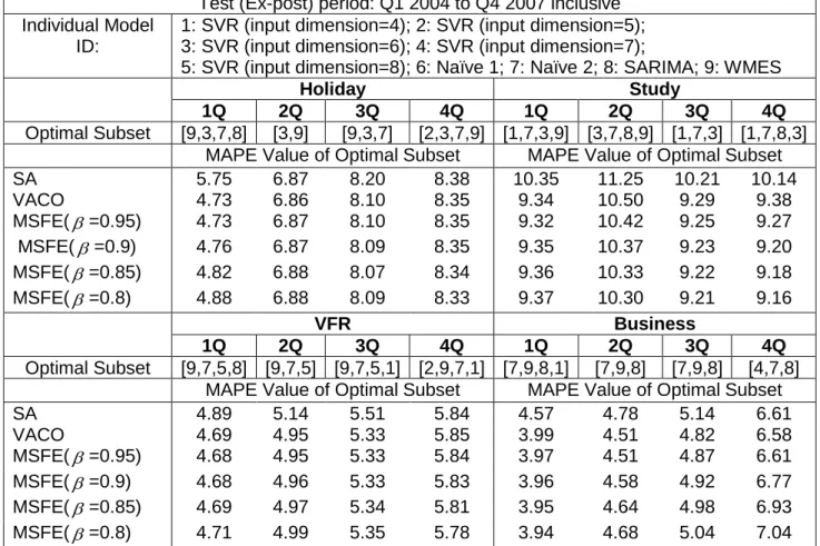
Table 2: MAPE values of optimal subsets for different linear combination methods Test (Ex-post) period: Q1 2004 to Q4 2007 inclusive Individual Model
ID:
1: SVR (input dimension=4); 2: SVR (input dimension=5); 3: SVR (input dimension=6); 4: SVR (input dimension=7);
5: SVR (input dimension=8); 6: Naïve 1; 7: Naïve 2; 8: SARIMA; 9: WMES
Holiday Study
1Q 2Q 3Q 4Q 1Q 2Q 3Q 4Q
Optimal Subset [9,3,7,8] [3,9] [9,3,7] [2,3,7,9] [1,7,3,9] [3,7,8,9] [1,7,3] [1,7,8,3] MAPE Value of Optimal Subset MAPE Value of Optimal Subset SA 5.75 6.87 8.20 8.38 10.35 11.25 10.21 10.14 VACO 4.73 6.86 8.10 8.35 9.34 10.50 9.29 9.38 MSFE( =0.95) 4.73 6.87 8.10 8.35 9.32 10.42 9.25 9.27 MSFE(=0.9) 4.76 6.87 8.09 8.35 9.35 10.37 9.23 9.20 MSFE( =0.85) 4.82 6.88 8.07 8.34 9.36 10.33 9.22 9.18 MSFE( =0.8) 4.88 6.88 8.09 8.33 9.37 10.30 9.21 9.16 VFR Business 1Q 2Q 3Q 4Q 1Q 2Q 3Q 4Q Optimal Subset [9,7,5,8] [9,7,5] [9,7,5,1] [2,9,7,1] [7,9,8,1] [7,9,8] [7,9,8] [4,7,8] MAPE Value of Optimal Subset MAPE Value of Optimal Subset SA 4.89 5.14 5.51 5.84 4.57 4.78 5.14 6.61 VACO 4.69 4.95 5.33 5.85 3.99 4.51 4.82 6.58 MSFE( =0.95) 4.68 4.95 5.33 5.84 3.97 4.51 4.87 6.61 MSFE( =0.9) 4.68 4.96 5.33 5.83 3.96 4.58 4.92 6.77 MSFE( =0.85) 4.69 4.97 5.34 5.81 3.95 4.64 4.98 6.93 MSFE( =0.8) 4.71 4.99 5.35 5.78 3.94 4.68 5.04 7.04
Note: optimal subset [9, 3, 7, 8] means that the ID numbers 9, 3, 7 and 8 of individual models are selected as optimal subset and used in the combination model. Q=quarter; SARIMA: Seasonal ARIMA; WMES: Winters’ multiplicative exponential smoothing
Table 3: MASE values of optimal subsets for different linear combination methods Test (Ex-post) period: Q1 2004 to Q4 2007 inclusive
Holiday Study
1Q 2Q 3Q 4Q 1Q 2Q 3Q 4Q
Optimal Subset [9,3,7,8] [3,9] [9,3,7] [2,3,7,9] [1,7,3,9] [3,7,8,9] [1,7,3] [1,7,8,3] MASE Value of Optimal Subset MASE Value of Optimal Subset SA 0.1554 0.1827 0.2143 0.2154 0.1617 0.1676 0.1602 0.1560 VACO 0.1296 0.1825 0.2124 0.2158 0.1479 0.1556 0.1469 0.1490 MSFE( =0.95) 0.1292 0.1826 0.2125 0.2164 0.1480 0.1551 0.1476 0.1485 MSFE( =0.9) 0.1300 0.1827 0.2121 0.2171 0.1485 0.1548 0.1482 0.1484 MSFE( =0.85) 0.1313 0.1828 0.2115 0.2180 0.1487 0.1547 0.1486 0.1486 MSFE( =0.8) 0.1328 0.1829 0.2118 0.2190 0.1489 0.1546 0.1490 0.1487 VFR Business 1Q 2Q 3Q 4Q 1Q 2Q 3Q 4Q Optimal Subset [9,7,5,8] [9,7,5] [9,7,5,1] [2,9,7,1] [7,9,8,1] [7,9,8] [7,9,8] [4,7,8] MASE Value of Optimal Subset MASE Value of Optimal Subset SA 0.3657 0.3755 0.3988 0.4325 0.5806 0.6058 0.6460 0.8237 VACO 0.3516 0.3611 0.3834 0.4316 0.5089 0.5722 0.6066 0.8265 MSFE( =0.95) 0.3511 0.3612 0.3832 0.4311 0.5056 0.5731 0.6123 0.8331 MSFE( =0.9) 0.3511 0.3615 0.3833 0.4303 0.5050 0.5808 0.6188 0.8550 MSFE( =0.85) 0.3516 0.3618 0.3837 0.4289 0.5041 0.5877 0.6261 0.8768 MSFE( =0.8) 0.3526 0.3631 0.3848 0.4271 0.5030 0.5931 0.6338 0.8919
17
Note: optimal subset [9,3,7,8] means that the ID numbers 9, 3, 7 and 8 of individual models are selected as optimal subset and used in the combination model. Q=quarter
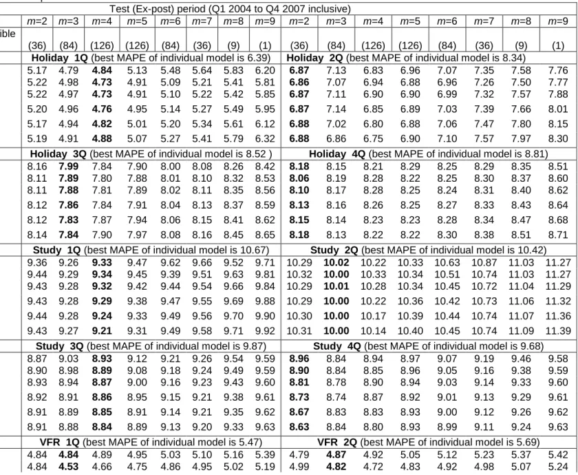
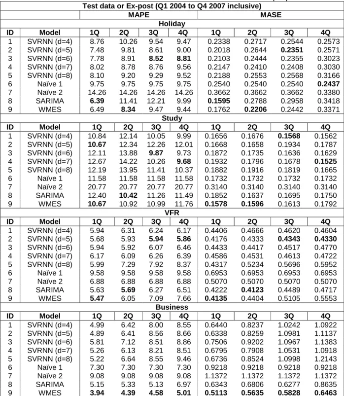
In order to validate the optimal subset selection approach, we compare the optimal subset selection results (MAPE and MASE values) with the results of the different linear combination methods using the test data for all possible combinations of m individual models (2m9). The MAPE and MASE values of all possible combinations with the best MAPE of the individual models are presented in Tables 4 and 5, respectively. The MAPE and MASE values of individual models are illustrated in Table A1 of Appendix.
18
Table 4: Best MAPE values for all possible combinations of m individual models on different combination methods Test (Ex-post) period (Q1 2004 to Q4 2007 inclusive)
m models m=2 m=3 m=4 m=5 m=6 m=7 m=8 m=9 m=2 m=3 m=4 m=5 m=6 m=7 m=8 m=9 Total number of all possible
combinations (36) (84) (126) (126) (84) (36) (9) (1) (36) (84) (126) (126) (84) (36) (9) (1) Combine Model Holiday 1Q (best MAPE of individual model is 6.39) Holiday 2Q (best MAPE of individual model is 8.34)
SA 5.17 4.79 4.84 5.13 5.48 5.64 5.83 6.20 6.87 7.13 6.83 6.96 7.07 7.35 7.58 7.76 VACO 5.22 4.98 4.73 4.91 5.09 5.21 5.41 5.81 6.86 7.07 6.94 6.88 6.96 7.26 7.50 7.77 MSFE(=0.95) 5.22 4.97 4.73 4.91 5.10 5.22 5.42 5.85 6.87 7.11 6.90 6.90 6.99 7.32 7.57 7.88 MSFE(=0.9) 5.20 4.96 4.76 4.95 5.14 5.27 5.49 5.95 6.87 7.14 6.85 6.89 7.03 7.39 7.66 8.01 MSFE(=0.85) 5.17 4.94 4.82 5.01 5.20 5.34 5.61 6.12 6.88 7.02 6.80 6.88 7.06 7.47 7.80 8.15 MSFE(=0.8) 5.19 4.91 4.88 5.07 5.27 5.41 5.79 6.32 6.88 6.86 6.75 6.90 7.10 7.57 7.97 8.30
Holiday 3Q (best MAPE of individual model is 8.52 ) Holiday 4Q (best MAPE of individual model is 8.81) SA 8.16 7.99 7.84 7.90 8.00 8.08 8.26 8.42 8.18 8.15 8.21 8.29 8.25 8.29 8.35 8.51 VACO 8.11 7.89 7.80 7.88 8.01 8.10 8.32 8.53 8.06 8.19 8.28 8.22 8.25 8.30 8.37 8.60 MSFE(=0.95) 8.11 7.88 7.81 7.89 8.02 8.11 8.35 8.56 8.10 8.17 8.28 8.25 8.24 8.31 8.40 8.62 MSFE(=0.9) 8.12 7.86 7.84 7.91 8.04 8.13 8.37 8.59 8.13 8.16 8.26 8.25 8.27 8.33 8.43 8.64 MSFE(=0.85) 8.12 7.83 7.87 7.94 8.06 8.15 8.41 8.62 8.15 8.14 8.23 8.23 8.28 8.34 8.47 8.68 MSFE(=0.8) 8.14 7.84 7.90 7.97 8.08 8.16 8.45 8.65 8.18 8.13 8.22 8.22 8.30 8.38 8.51 8.71
Study 1Q (best MAPE of individual model is 10.67) Study 2Q (best MAPE of individual model is 10.42) SA 9.36 9.26 9.33 9.47 9.62 9.66 9.52 9.71 10.29 10.02 10.22 10.33 10.63 10.87 11.03 11.27 VACO 9.44 9.29 9.34 9.45 9.39 9.51 9.63 9.81 10.32 10.00 10.33 10.34 10.51 10.74 11.03 11.27 MSFE(=0.95) 9.43 9.28 9.32 9.42 9.44 9.54 9.66 9.84 10.29 10.01 10.28 10.34 10.45 10.72 11.04 11.29 MSFE(=0.9) 9.43 9.28 9.29 9.38 9.47 9.55 9.69 9.88 10.29 10.00 10.22 10.36 10.42 10.73 11.06 11.32 MSFE(=0.85) 9.44 9.28 9.24 9.33 9.49 9.56 9.70 9.90 10.30 10.00 10.17 10.39 10.44 10.74 11.07 11.36 MSFE(=0.8) 9.43 9.27 9.21 9.31 9.49 9.58 9.71 9.92 10.31 10.00 10.14 10.40 10.45 10.74 11.09 11.39
Study 3Q (best MAPE of individual model is 9.87) Study 4Q (best MAPE of individual model is 9.68) SA 8.87 9.03 8.93 9.12 9.21 9.26 9.54 9.59 8.96 8.84 8.94 8.97 9.07 9.19 9.46 9.58 VACO 8.90 8.98 8.89 9.08 9.18 9.24 9.49 9.59 8.90 8.84 8.85 8.96 9.05 9.16 9.38 9.59 MSFE(=0.95) 8.93 8.94 8.87 9.00 9.16 9.23 9.43 9.60 8.81 8.78 8.90 8.94 9.03 9.14 9.33 9.60 MSFE(=0.9) 8.92 8.91 8.86 8.95 9.15 9.21 9.38 9.61 8.73 8.74 8.87 8.92 9.01 9.13 9.29 9.61 MSFE(=0.85) 8.91 8.89 8.85 8.91 9.14 9.21 9.35 9.62 8.67 8.83 8.83 8.93 9.00 9.12 9.26 9.62 MSFE(=0.8) 8.91 8.88 8.84 8.89 9.13 9.20 9.33 9.63 8.63 8.84 8.80 8.93 8.99 9.11 9.24 9.63
VFR 1Q (best MAPE of individual model is 5.47) VFR 2Q (best MAPE of individual model is 5.69) SA 4.84 4.84 4.89 4.95 5.03 5.10 5.16 5.39 4.79 4.87 4.92 5.05 5.12 5.23 5.37 5.42 VACO 4.84 4.53 4.66 4.75 4.86 4.95 5.02 5.19 4.99 4.82 4.72 4.83 4.92 4.98 5.07 5.24
19
MSFE(=0.95) 4.84 4.53 4.66 4.75 4.85 4.94 5.02 5.18 5.00 4.80 4.75 4.85 4.94 4.99 5.09 5.24 MSFE(=0.9) 4.84 4.54 4.67 4.76 4.87 4.95 5.02 5.18 5.00 4.75 4.81 4.88 4.96 5.02 5.14 5.26 MSFE(=0.85) 4.84 4.56 4.69 4.80 4.89 4.97 5.05 5.19 4.95 4.78 4.82 4.92 4.99 5.08 5.21 5.27 MSFE(=0.8) 4.84 4.59 4.70 4.83 4.92 5.00 5.08 5.23 4.87 4.81 4.85 4.97 5.03 5.14 5.25 5.31
VFR 3Q (best MAPE of individual model is 5.94) VFR 4Q (best MAPE of individual model is 5.86) SA 5.80 5.46 5.43 5.48 5.57 5.63 5.72 5.73 6.02 5.86 5.78 5.82 5.86 5.92 6.11 6.21 VACO 5.84 5.46 5.32 5.36 5.41 5.47 5.53 5.70 5.96 5.95 5.85 5.83 5.87 5.92 6.04 6.22 MSFE(=0.95) 5.83 5.45 5.32 5.36 5.41 5.48 5.54 5.68 5.95 5.94 5.84 5.82 5.86 5.92 6.04 6.20 MSFE(=0.9) 5.83 5.42 5.32 5.37 5.43 5.49 5.55 5.67 5.94 5.92 5.83 5.81 5.85 5.91 6.03 6.17 MSFE(=0.85) 5.81 5.40 5.32 5.38 5.46 5.51 5.58 5.65 5.91 5.90 5.79 5.79 5.84 5.92 6.04 6.13 MSFE(=0.8) 5.82 5.39 5.34 5.39 5.47 5.55 5.61 5.64 5.88 5.81 5.76 5.77 5.86 5.95 6.03 6.09
Business 1Q (best MAPE of individual model is 3.94) Business 2Q (best MAPE of individual model is 4.39) SA 4.13 4.10 4.18 4.28 4.20 4.19 4.33 4.43 4.68 4.78 4.76 5.03 5.24 5.41 5.60 5.76 VACO 4.22 4.06 3.99 4.06 4.21 4.38 4.51 4.71 4.65 4.51 4.98 5.34 5.56 5.70 5.86 6.03 MSFE(=0.95) 4.22 4.06 3.97 4.07 4.23 4.40 4.53 4.72 4.63 4.51 5.07 5.42 5.62 5.77 5.93 6.09 MSFE(=0.9) 4.20 4.05 3.96 4.08 4.24 4.41 4.54 4.74 4.59 4.58 5.16 5.48 5.67 5.81 5.97 6.13 MSFE(=0.85) 4.16 4.04 3.95 4.08 4.24 4.41 4.55 4.75 4.54 4.64 5.22 5.53 5.71 5.84 6.01 6.16 MSFE(=0.8) 4.13 4.02 3.94 4.07 4.24 4.41 4.55 4.75 4.48 4.68 5.25 5.56 5.73 5.86 6.02 6.18
Business 3Q (best MAPE of individual model is 4.58) Business 4Q (best MAPE of individual model is 5.01) SA 4.52 4.98 5.33 5.68 6.03 6.28 6.52 6.75 5.69 5.96 6.17 6.26 6.39 6.68 6.93 7.18 VACO 4.56 4.82 5.40 6.02 6.46 6.79 7.06 7.27 6.07 6.25 6.27 6.44 6.86 7.19 7.44 7.64 MSFE(=0.95) 4.55 4.87 5.48 6.17 6.61 6.94 7.20 7.39 6.09 6.32 6.34 6.57 7.02 7.33 7.59 7.78 MSFE(=0.9) 4.54 4.92 5.56 6.27 6.73 7.06 7.31 7.49 6.10 6.37 6.39 6.70 7.15 7.45 7.70 7.89 MSFE(=0.85) 4.52 4.98 5.63 6.34 6.82 7.15 7.38 7.55 6.09 6.40 6.40 6.76 7.24 7.53 7.78 7.97 MSFE(=0.8) 4.50 5.04 5.69 6.38 6.87 7.21 7.43 7.59 6.06 6.42 6.40 6.81 7.30 7.58 7.84 8.01
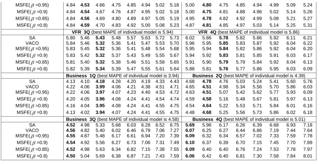
Table 5: Best MASE values for all possible combinations of m individual models on different combination methods Test (Ex-post) period (Q1 2004 to Q4 2007 inclusive)
m models m=2 m=3 m=4 m=5 m=6 m=7 m=8 m=9 m=2 m=3 m=4 m=5 m=6 m=7 m=8 m=9 Total number of all
possible combinations
(36) (84) (126) (126) (84) (36) (9) (1) (36) (84) (126) (126) (84) (36) (9) (1) Combine Model Holiday 1Q (best MASE of individual model is 0.1595) Holiday 2Q (best MASE of individual model is 0.2206)
SA 0.1356 0.1249 0.1262 0.1340 0.1434 0.1494 0.1530 0.1619 0.1827 0.1844 0.1803 0.1844 0.1867 0.1923 0.1975 0.2024 VACO 0.1355 0.1301 0.1263 0.1285 0.1335 0.1384 0.1425 0.1518 0.1825 0.1892 0.1816 0.1827 0.1838 0.1900 0.1965 0.2024 MSFE(=0.95) 0.1355 0.1300 0.1264 0.1291 0.1341 0.1386 0.1427 0.1527 0.1826 0.1882 0.1810 0.1830 0.1846 0.1913 0.1982 0.2054
20
MSFE(=0.9) 0.1355 0.1292 0.1265 0.1304 0.1360 0.1395 0.1440 0.1551 0.1827 0.1854 0.1806 0.1826 0.1856 0.1929 0.2003 0.2090 MSFE(=0.85) 0.1355 0.1287 0.1269 0.1322 0.1386 0.1409 0.1469 0.1598 0.1828 0.1824 0.1799 0.1820 0.1866 0.1948 0.2041 0.2130 MSFE(=0.8) 0.1368 0.1280 0.1287 0.1342 0.1400 0.1424 0.1514 0.1650 0.1829 0.1795 0.1792 0.1827 0.1876 0.1968 0.2083 0.2171
Holiday 3Q (best MASE of individual model is 0.2351) Holiday 4Q (best MASE of individual model is 0.2437)
SA 0.2169 0.2095 0.2067 0.2064 0.2098 0.2104 0.2158 0.2138 0.2142 0.2154 0.2136 0.2145 0.2169 0.2197 0.2235 0.2138 VACO 0.2142 0.2078 0.2079 0.2080 0.2084 0.2118 0.2184 0.2113 0.2149 0.2156 0.2128 0.2156 0.2182 0.2210 0.2263 0.2113 MSFE(=0.95) 0.2142 0.2077 0.2079 0.2085 0.2088 0.2121 0.2190 0.2121 0.2147 0.2152 0.2128 0.2157 0.2186 0.2217 0.2269 0.2121 MSFE(=0.9) 0.2142 0.2071 0.2079 0.2086 0.2095 0.2127 0.2200 0.2127 0.2143 0.2146 0.2127 0.2163 0.2192 0.2227 0.2278 0.2127 MSFE(=0.85) 0.2142 0.2064 0.2086 0.2089 0.2104 0.2134 0.2210 0.2133 0.2140 0.2138 0.2126 0.2163 0.2198 0.2239 0.2288 0.2133 MSFE(=0.8) 0.2143 0.2062 0.2090 0.2092 0.2114 0.2143 0.2219 0.2139 0.2137 0.2145 0.2126 0.2164 0.2211 0.2253 0.2299 0.2139
Study 1Q (best MASE of individual model is 0.1578) Study 2Q (best MASE of individual model is 0.1596)
SA 0.1466 0.1468 0.1484 0.1507 0.1526 0.1520 0.1508 0.1534 0.1546 0.1532 0.1552 0.1572 0.1602 0.1614 0.1631 0.1659 VACO 0.1480 0.1471 0.1475 0.1488 0.1492 0.1514 0.1531 0.1554 0.1541 0.1527 0.1545 0.1573 0.1576 0.1601 0.1635 0.1674 MSFE(=0.95) 0.1479 0.1466 0.1463 0.1486 0.1499 0.1518 0.1535 0.1559 0.1532 0.1523 0.1523 0.1567 0.1571 0.1600 0.1636 0.1678 MSFE(=0.9) 0.1480 0.1468 0.1458 0.1483 0.1503 0.1521 0.1538 0.1564 0.1528 0.1520 0.1519 0.1561 0.1569 0.1602 0.1639 0.1683 MSFE(=0.85) 0.1479 0.1466 0.1458 0.1480 0.1506 0.1523 0.1541 0.1567 0.1527 0.1518 0.1516 0.1558 0.1572 0.1603 0.1642 0.1689 MSFE(=0.8) 0.1476 0.1465 0.1457 0.1479 0.1506 0.1524 0.1543 0.1570 0.1527 0.1518 0.1514 0.1557 0.1573 0.1604 0.1644 0.1693
Study 3Q (best MASE of individual model is 0.1568) Study 4Q (best MASE of individual model is 0.1525)
SA 0.1442 0.1470 0.1469 0.1458 0.1465 0.1479 0.1495 0.1515 0.1452 0.1464 0.1447 0.1429 0.1442 0.1452 0.1484 0.1503 VACO 0.1441 0.1431 0.1431 0.1447 0.1475 0.1487 0.1505 0.1534 0.1458 0.1440 0.1447 0.1456 0.1467 0.1477 0.1494 0.1520 MSFE(=0.95) 0.1438 0.1422 0.1433 0.1445 0.1472 0.1489 0.1503 0.1538 0.1459 0.1440 0.1446 0.1459 0.1470 0.1478 0.1493 0.1524 MSFE(=0.9) 0.1440 0.1430 0.1435 0.1443 0.1471 0.1490 0.1502 0.1542 0.1459 0.1440 0.1449 0.1462 0.1472 0.1479 0.1491 0.1527 MSFE(=0.85) 0.1440 0.1436 0.1436 0.1442 0.1470 0.1490 0.1501 0.1546 0.1435 0.1440 0.1451 0.1464 0.1473 0.1480 0.1491 0.1530 MSFE(=0.8) 0.1439 0.1436 0.1437 0.1442 0.1469 0.1492 0.1500 0.1549 0.1423 0.1443 0.1453 0.1465 0.1475 0.1481 0.1490 0.1533
VFR 1Q (best MASE of individual model is 0.4135) VFR 2Q (best MASE of individual model is 0.4123)
SA 0.3661 0.3597 0.3626 0.3695 0.3743 0.3783 0.3829 0.3990 0.3512 0.3504 0.3585 0.3691 0.3734 0.3827 0.3926 0.3964 VACO 0.3663 0.3444 0.3476 0.3529 0.3601 0.3671 0.3732 0.3843 0.3659 0.3497 0.3417 0.3505 0.3563 0.3620 0.3693 0.3817 MSFE(=0.95) 0.3662 0.3447 0.3479 0.3528 0.3598 0.3671 0.3729 0.3836 0.3661 0.3486 0.3442 0.3522 0.3580 0.3630 0.3713 0.3823 MSFE(=0.9) 0.3661 0.3456 0.3486 0.3539 0.3609 0.3683 0.3734 0.3834 0.3653 0.3478 0.3469 0.3542 0.3602 0.3652 0.3751 0.3833 MSFE(=0.85) 0.3661 0.3473 0.3494 0.3564 0.3633 0.3698 0.3748 0.3843 0.3630 0.3466 0.3509 0.3571 0.3624 0.3700 0.3802 0.3847 MSFE(=0.8) 0.3662 0.3493 0.3502 0.3595 0.3660 0.3718 0.3768 0.3872 0.3569 0.3453 0.3540 0.3633 0.3653 0.3752 0.3836 0.3879
VFR 3Q (best MASE of individual model is 0.4343) VFR 4Q (best MASE of individual model is 0.4330)
SA 0.4157 0.3912 0.3886 0.3958 0.4035 0.4101 0.4125 0.4157 0.4467 0.4301 0.4227 0.4276 0.4314 0.4361 0.4477 0.4546 VACO 0.4192 0.3919 0.3834 0.3871 0.3903 0.3942 0.3994 0.4116 0.4420 0.4381 0.4284 0.4276 0.4316 0.4344 0.4416 0.4546 MSFE(=0.95) 0.4191 0.3911 0.3832 0.3870 0.3909 0.3945 0.4000 0.4106 0.4414 0.4382 0.4280 0.4272 0.4312 0.4342 0.4412 0.4532 MSFE(=0.9) 0.4188 0.3893 0.3833 0.3877 0.3912 0.3958 0.4015 0.4095 0.4405 0.4375 0.4266 0.4267 0.4304 0.4341 0.4410 0.4512 MSFE(=0.85) 0.4185 0.3875 0.3837 0.3877 0.3919 0.3983 0.4040 0.4086 0.4390 0.4337 0.4240 0.4265 0.4300 0.4346 0.4422 0.4488 MSFE(=0.8) 0.4191 0.3864 0.3848 0.3896 0.3942 0.4012 0.4067 0.4084 0.4370 0.4262 0.4223 0.4258 0.4304 0.4372 0.4430 0.4462
21
Business 1Q (best MASE of individual model is 0.5113) Business 2Q (best MASE of individual model is 0.5635)
SA 0.5354 0.5223 0.5349 0.5447 0.5370 0.5373 0.5559 0.5672 0.5978 0.6058 0.6056 0.6421 0.6698 0.6917 0.7164 0.7357 VACO 0.5372 0.5203 0.5089 0.5218 0.5396 0.5620 0.5790 0.6050 0.5949 0.5722 0.6376 0.6854 0.7132 0.7318 0.7504 0.7728 MSFE(=0.95) 0.5352 0.5200 0.5056 0.5231 0.5419 0.5645 0.5816 0.6075 0.5916 0.5731 0.6501 0.6955 0.7214 0.7396 0.7585 0.7803 MSFE(=0.9) 0.5329 0.5193 0.5050 0.5242 0.5432 0.5660 0.5834 0.6093 0.5865 0.5808 0.6612 0.7037 0.7279 0.7455 0.7645 0.7860 MSFE(=0.85) 0.5296 0.5181 0.5041 0.5245 0.5442 0.5665 0.5842 0.6105 0.5800 0.5877 0.6676 0.7100 0.7327 0.7497 0.7686 0.7900 MSFE(=0.8) 0.5270 0.5166 0.5030 0.5239 0.5441 0.5661 0.5842 0.6109 0.5727 0.5931 0.6715 0.7142 0.7357 0.7521 0.7709 0.7924
Business 3Q (best MASE of individual model is 0.5828) Business 4Q (best MASE of individual model is 0.6463)
SA 0.5664 0.6291 0.6702 0.7142 0.7615 0.7961 0.8294 0.8593 0.7148 0.7478 0.7753 0.7859 0.8062 0.8450 0.8786 0.9117 VACO 0.5691 0.6066 0.6772 0.7613 0.8200 0.8635 0.9001 0.9287 0.7592 0.7824 0.7893 0.8110 0.8679 0.9122 0.9461 0.9734 MSFE(=0.95) 0.5686 0.6123 0.6876 0.7806 0.8395 0.8835 0.9180 0.9447 0.7617 0.7912 0.7945 0.8295 0.8887 0.9319 0.9661 0.9919 MSFE(=0.9) 0.5677 0.6188 0.6973 0.7926 0.8554 0.8996 0.9320 0.9573 0.7625 0.7978 0.7966 0.8444 0.9060 0.9475 0.9817 1.0064 MSFE(=0.85) 0.5663 0.6261 0.7065 0.8018 0.8670 0.9114 0.9419 0.9662 0.7612 0.8022 0.7978 0.8530 0.9190 0.9585 0.9925 1.0167 MSFE(=0.8) 0.5644 0.6338 0.7136 0.8079 0.8741 0.9188 0.9476 0.9714 0.7575 0.8047 0.7983 0.8586 0.9263 0.9652 0.9989 1.0229 Note: SA: Simple Average; VACO: Variance-Covariance; DMSFE(): Discounted Mean Square Forecast Error method with different, respectively.
m: The number of individual models for the combination, Bold denotes the best performance of combinations with m (2m9) individual models among all possible combinations models. Bold values corresponding to the best m. Q=quarter.
22
We can observe that the MAPE values presented in Tables 2 and 4 and the MASE values presented in Tables 3 and 5 for the combination of optimal subsets are significantly smaller than the best individual models for most cases apart from the business purpose of visit. If we use MAPE as an error measurement, only the cases which are the SA method for Q2-Q4 and the VACO method for Q2 at the study purpose of visit underperform the best individual models. If we use MASE as an error measurement, only the cases which are the SA method for Q1-Q4 of the study purpose of visit underperform the best individual models. The worst linear combination method is SA for this study. There are 72 cases (3X4X6=72) which are constructed by 3 purposes (holiday, study and VFR), 4 quarters (Q1-Q4), and 6 linear combination methods. There are only 4 out of 72 cases that the proposed combination model underperforms the best individual models. Therefore, the percentage of optimal subsets outperforming the best individual models is 94.4% (68 out of 72 cases) for all linear combinations and all purposes of visits except the business purpose of visit for both MAPE and MASE error measurements. For the business purpose of visit, the best individual model gives better performance than any subset of individual models that contains more than one individual model.
Tables 4 and 5 show that the combinations of two-four individual models give the best performance for all purposes of visits, which is similar to the results of applying the MI algorithm for optimal subset selection. These validate the results in the paper (Shen, Li & Song, 2011). Shen, Li and Song suggested that the highest frequencies of the best combination forecasts appear when the minimum number of individual models for the combination is two. This is unlikely to be effective if a combination of more than five individual forecasts.
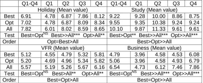
The subset of individual models that gives the best performance among all possible combinations of individual models is called the best subset. In order to validate the optimal subset which is obtained using the MI algorithm, the Mann-Whitney test is employed, because the MAPE and MASE values do not satisfy normal distribution by using the Kolmogorov-Smirnov normality test. The results of Mann-Whitney tests and the mean values of MAPE and MASE for all linear combination methods except the SA method are presented in Tables 6 and 7 for the different sets of individual models. These different sets of individual models are the ‘set of all individual models’ (All), the ‘best subset’ (Best) presented in Tables 4 and 5 and the ‘optimal subset’ (Opt) presented in Table 2 and 3 at different purpose of visits. ‘=’, ‘>’ and ‘>>’ in Tables 6 and 7 indicate non statistically significant (equally performance), statistically significant at 5% (performance better than), and very statistically significant at 1% (performance much better than), respectively.
23
Table 6: Mann-Whitney test to MAPE values for all linear combination methods (except SA)
Q1-Q4 Q1 Q2 Q3 Q4 Q1-Q4 Q1 Q2 Q3 Q4
Holiday (Mean value) Study (Mean value)
Best 6.91 4.78 6.87 7.86 8.12 9.22 9.28 10.00 8.86 8.75
Opt 7.02 4.78 6.87 8.09 8.34 9.55 9.35 10.38 9.24 9.24
All 7.82 6.01 8.02 8.59 8.65 10.10 9.87 11.33 9.61 9.61 Test Best=OptNS Best>>All*** Opt>All** Best>Opt** Best>>All*** Opt>>All***
Order Opt=Best>All Best>Opt>>All
VFR (Mean value) Business (Mean value)
Best 5.12 4.55 4.79 5.32 5.81 4.79 3.96 4.58 4.53 6.08
Opt 5.20 4.69 4.96 5.34 5.82 5.06 3.96 4.58 4.93 6.79
All 5.57 5.19 5.26 5.67 6.16 6.54 4.73 6.12 7.46 7.86
Test Best=OptNS Best>All** Opt>All** Best=OptNS Best>>All*** Opt>>All***
Order Best=Opt>All Best=Opt>>All
***: Statistical significant difference at 1% level; **: Statistical significant difference at 5% level; NS: No statistical significant difference; Q=quarter.
Table 7: Mann-Whitney test to MASE values for all linear combination methods (except SA) Q1-Q4 Q1 Q2 Q3 Q4 Q1-Q4 Q1 Q2 Q3 Q4
Holiday (Mean value) Study (Mean value)
Best 0.1824 0.1270 0.1827 0.2070 0.2127 0.1464 0.1462 0.1521 0.1431 0.1441 Opt 0.1857 0.1306 0.1827 0.2121 0.2173 0.1500 0.1484 0.1550 0.1481 0.1486 All 0.1979 0.1569 0.2094 0.2127 0.2127 0.1579 0.1563 0.1683 0.1542 0.1527 Test Best=OptNS Best>All** Opt=AllNS Best>Opt** Best>>All*** Opt>>All*** Order Best=Opt>=All Best>Opt>>All
VFR (Mean value) Business (Mean value)
Best 0.3759 0.3463 0.3476 0.3837 0.4259 0.6045 0.5053 0.5851 0.5672 0.7604 Opt 0.3817 0.3516 0.3617 0.3837 0.4298 0.6407 0.5053 0.5814 0.6195 0.8567 All 0.4073 0.3846 0.3840 0.4097 0.4508 0.8372 0.6086 0.7843 0.9537 1.0023 Test Best:OptNS Best:All*** Opt:All*** Best:OptNS Best:All*** Opt:All*** Order Best=Opt>>All Best=Opt>>All
Note: ***: Statistical significant difference at 1% level; **: Statistical significant difference at 5% level; NS: No statistical significant difference; Q=quarter
From Tables 6 and 7, we can see that the performance of the optimal sets is significantly better than that of the set that contains all individual models except holiday purpose with the MASE measurement, and no statistical significant difference with the best subset except one case (study). The optimal subset of individual models gives good enough performance, but not necessarily the best performance among all possible combinations of individual models. This suggests that we can use an optimal subset of individual models instead of all individual models in forecasting. The results of Tables 2, 3, 6 and 7 are suggesting following:
The optimal subset selection from individual models using the MI algorithm shows robust and good performance in general. However, optimal subset selection using the MI algorithm does not guarantee that the optimal subset is the same as the best subset.