IMES DISCUSSION PAPER SERIES
INSTITUTE FOR MONETARY AND ECONOMIC STUDIES
BANK OF JAPAN
2-1-1 NIHONBASHI-HONGOKUCHO CHUO-KU, TOKYO 103-8660
JAPAN
You can download this and other papers at the IMES Web site:
http://www.imes.boj.or.jp
Do not reprint or reproduce without permission.
The Effects of Monetary Policy Commitment:
Evidence from Time-varying Parameter VAR Analysis
Jouchi Nakajima, Shigenori Shiratsuka, and Yuki Teranishi
NOTE: IMES Discussion Paper Series is circulated in
order to stimulate discussion and comments. Views
expressed in Discussion Paper Series are those of
authors and do not necessarily reflect those of
the Bank of Japan or the Institute for Monetary
and Economic Studies.
IMES Discussion Paper Series 2010-E-6
March 2010
The Effects of Monetary Policy Commitment:
Evidence from Time-varying Parameter VAR Analysis
Jouchi Nakajima*, Shigenori Shiratsuka**, and Yuki Teranishi***
Abstract
In this paper, we explore the effects of the Bank of Japan's (BOJ's) policy
commitment under zero interest rates on the economy, by considering the
transmission channel of altering private-sector expectations. To that end, we carry
out a structural vector autoregression analysis on macroeconomic variables and
private-sector expectations variables, using a time-varying parameters estimation
technique with stochastic volatility. We show empirical evidence on two points.
First, the BOJ's policy commitment regarding the future course of short-term
interest rates, associated with only a small reduction in policy interest rates,
succeeded in altering private-sector expectations. Second, the BOJ's policy
commitment alone, nevertheless, was not sufficient to restore the previous trends in
prices and output.
Keywords: Policy commitment; policy duration effect; expectations management;
Bayesian estimation; time-varying parameter vector autoregression with
stochastic volatility
JEL classification: C11; C13; E43; E44; E52; E58
*Currently in the Personnel and Corporate Affairs Department (studying at Duke University, E-mail: [email protected])
**Deputy Director-General, Institute for Monetary and Economic Studies, Bank of Japan (E-mail: [email protected])
***Associate Director, Institute for Monetary and Economic Studies, Bank of Japan (E-mail: [email protected])
We thank Kazuo Ueda, Tsutomu Watanabe, Kosuke Aoki, and seminar participants at the Bank of Japan for their useful comments. Views expressed in this paper are those of the authors and do not necessarily reflect the official views of the Bank of Japan.
1
Introduction
In this paper, we explore the e¤ect of the Bank of Japan’s (BOJ’s) policy commitment
under zero interest rates on the economy, by considering of the transmission channel of
altering private-sector expectations. To that end, we carry out a structural vector
au-toregression (VAR) analysis on macroeconomic variables and private-sector expectations
variables, using a time-varying parameters estimation technique with stochastic volatility. As highlighted by Woodford (2005), a central bank can in‡uence economic activity by
shaping private-sector expectations about the future course of the economy, including
short-term interest rates. A central bank thus needs to consider how to manage the expectations
in a more e¤ective way when mapping its monetary policy strategy. In particular, when
interest rates are at or near zero, a central bank needs to communicate to the public about
the duration that the current extremely low interest rates will be maintained. Using a
theoretical model, Eggertsson and Woodford (2003) and Jung, Teranishi, and Watanabe
(2005) show that by committing to the future zero interest rates in advance a central bank can lower long-term interest rates, and so lower the real interest rate thanks to the
in‡ation expectation to mitigate the de‡ationary shock. Such a mechanism is often called
the “policy duration e¤ect,” as in Fujiki, Okina, and Shiratsuka (2001).
The BOJ has two episodes of policy commitment under zero interest rates: the zero
interest rate policy (ZIRP) from February 12, 1999 to August 11, 2000 and the quantitative
easing policy (QEP) from March 19, 2001 to March 9, 2006, as summarized in Table 1.1
Under the ZIRP, the BOJ started lowering the overnight call rate initially to around 0.15
percent in February 1999, and subsequently induced a further decline to 0.02 percent in view of market developments. In addition, the BOJ Governor at the time, Masaru Hayami,
announced at a press conference in April 1999 that the BOJ would continue zero interest
rates “until the de‡ationary concerns were dispelled.”Under the QEP, the BOJ also made a
1Such a monetary policy commitment is not restricted to Japan. The Federal Reserve, for example,
made an unconditional commitment in the summer of 2003 by using so-called forward-looking language: “policy accommodation can be maintained for a considerable period.” In that context, Levinet al. (2009) describe such policy measures as “forward guidance.”
commitment to targeting the current account balances at the BOJ “until the core consumer
price in‡ation becomes stably zero or above.”2
The empirical validity of the policy duration e¤ect implied by theoretical studies is still
an open question. In that context, Ugai (2007) concludes in his comprehensive survey on empirical studies on the e¤ects of the QEP that the e¤ects of expanding the monetary base
and altering the composition of the BOJ’s balance sheet, if any, are generally smaller than
those stemming from the policy commitment.
More speci…cally, Fujiki and Shiratsuka (2002) and Okina and Shiratsuka (2004a)
fo-cus on the response of the yield curve. They conclude that the policy duration e¤ect was
highly e¤ective in stabilizing market expectations regarding the future path of short-term
interest rates, although it failed to reverse de‡ationary expectations in the …nancial
mar-kets, since monetary policy alone could not reverse de‡ation, coupled with low economic growth. Such easing e¤ects were not transmitted throughout the economy in Japan, since
the transmission channel linking the …nancial and non…nancial sectors remained blocked.
However, their analysis covers only the …nancial markets using high-frequency data.
Oda and Ueda (2005) employ a macro-…nance approach and conclude that the BOJ’s
monetary policy since 1999 functioned mainly through the zero interest rate commitment,
which led to declines in medium- to long-term interest rates. They also note that the
portfolio rebalancing e¤ect was not found to be signi…cant. Kimura et al. (2003) apply
Bayesian VAR analysis to examine the expansionary e¤ect of the increase in the monetary
base on the economy in the QEP, which includes the policy duration e¤ect and portfolio rebalancing e¤ect. They conclude that although it is di¢ cult to deny the possibility that
such a positive e¤ect induced a change in the portfolios of economic agents and ultimately
2The BOJ started releasing Board Members’projections on …scal year averages of real economic growth
and in‡ation (overall CGPI and core CPI) in October 2000. Projection period was initially just for the current …scal year, but were gradually extended: from October 2001, October projection included the aver-age …gures for economic growth and in‡ation in the next …scal year, and from April 2005, April projection also included …gures for the next …scal year. In addition, in April 2008, the BOJ started releasing the distribution of Board Members’projections, as risk-balance charts. In July 2008, the BOJ started releasing projections at the interim assessment in January and July, and decided to extend the projection period for one more year until the two …scal years ahead from October 2008.
stimulated economic activity, the possibility is highly uncertain and very small at best.
In this paper, we apply a time-varying parameter VAR (TVP-VAR) model with
sto-chastic volatility, thereby examining structural changes in macroeconomic dynamics,
in-cluding interaction with private-sector expectations. In that context, we should note that stochastic volatility in disturbances plays an important role in improving the estimation
precision for the sample period including extremely low interest rates. We have two main
…ndings. First, the BOJ’s policy commitment regarding the future course of short-term
interest rates, associated with only a small reduction in policy interest rates, succeeded in
changing private-sector expectations in the household and business sectors. Second, the
BOJ’s policy commitment alone, nevertheless, was not su¢ cient to restore the previous
trends in prices and output. That suggests that the monetary policy commitment was not
a cure-all measure for structural impediments that induced downward shifts in the trend growth path.
This paper is structured as follows. In Section 2, we explain our empirical framework:
a VAR model employing a time-varying parameters technique with stochastic volatility as
well as data used in the estimation. In Section 3, we show our empirical results for the e¤ect
of the policy commitment regarding the interaction between macroeconomic variables and
private-sector expectations variables. In Section 4, we conclude the paper.
2
Empirical Framework
In this section, we explain our empirical framework: a VAR estimation using a time-varying parameters technique with stochastic volatility as well as data used in the estimation.
2.1 Time-varying parameter VAR model with stochastic volatility
To introduce the TVP-VAR model with stochastic volatility, we begin with a basic
struc-tural VAR model de…ned as
where yt is a k 1 vector of observed variables, and A, F1; : : : ; Fs are k k matrices of
coe¢ cients.3 The disturbanceutis ak 1structural shock and we assumeut N(0; ),
where = 0 B B B B B B @ 1 0 0 0 . .. ... ... .. . . .. ... 0 0 0 k 1 C C C C C C A :
We then specify the simultaneous relations of the structural shock by recursive
identi…ca-tion, assuming that A is lower-triangular,
A = 0 B B B B B B @ 1 0 0 a21 . .. . .. ... .. . . .. . .. 0 ak1 ak;k 1 1 1 C C C C C C A :
We rewrite equation (1) as the following reduced-form SVAR model:
yt=B1yt 1+ +Bsyt s+A 1 "t; "t N(0; Ik);
where Bi =A 1Fi, for i= 1; : : : ; s. Stacking the elements in the rows of the Bi’s to form
(k2s 1vector), and de…ningXt=Ik (yt0 1; : : : ;y0t k), where denotes the Kronecker
product, the model can be written as
yt = Xt +A 1 "t; t=s+ 1; : : : ; n: (2)
Now, all parameters in equation (2) are time-invariant. We extend it to the TVP-VAR
model with stochastic volatility by allowing the parameters to vary over time, following
Primiceri (2005).
Consider now the TVP-VAR with stochastic volatility speci…ed by
yt = Xt t+At1 t"t; t=s+ 1; : : : ; n; (3)
3
where the coe¢ cients t, the parametersAt, and tare all time varying. There are many
ways to model the process for those time-varying parameters.
Now letat= (a21; a31; a32; a41,: : : ; ak;k 1)0 be a stacked vector of the lower-triangular
elements inAtandht= (h1t; : : : ; hkt)0 withhjt = log 2jt, forj = 1; : : : ; k,t=s+ 1; : : : ; n.
We assume that the parameters in equation (3) follow a random-walk process as follows:
t+1 = t+u t; at+1 = at+uat; ht+1 = ht+uht; 0 B B B B B B @ "t u t uat uht 1 C C C C C C A N 0 B B B B B B @ 0; 0 B B B B B B @ I O O O O O O O O a O O O O h 1 C C C C C C A 1 C C C C C C A ; fort=s+1; : : : ; n, where s+1 N( 0; 0),as+1 N( a0; a0)andhs+1 N( h0; h0).
The TVP-VAR model, combined with stochastic volatility, enables us to take a very
‡exible and robust speci…cation of parameters to capture the potential time-varying nature
of the underlying structure.
2.2 Estimation methodology
The TVP-VAR model can be estimated using the Markov chain Monte Carlo (MCMC)
method in the context of a Bayesian inference, even though the likelihood function of
the model is intractable.4 The following priors are assumed for the i-th diagonals of the covariance matrices: ( )i 2 Gamma(40;0:02), ( a)i 2 Gamma(4;0:02), and
( h)i 2 Gamma(4;0:02). For the initial state of the time-varying parameter, the
follow-ing priors are set as
0 = a0 = h0 = 0, and 0 = a0 = h0 = 10 I. To compute the
posterior estimates, we draw 10;000samples after the initial 1,000 samples are discarded.
2.3 Data
We employ four categories of data on a quarterly basis. The …rst category corresponds
to general prices: the consumer price index (CPI) and the corporate goods price index
(CGPI) for the business sector. The CPI is a core indicator, excluding volatile components
4
of perishables from the headline, while the CGPI is a headline indicator. The second
is output measures for real GDP and investment in the National Accounts. The third is
interest rates: the overnight call rate for short-term interest rates and the …ve-year Japanese
government bond (JGB) yield for long-term interest rates. The fourth corresponds to indicators for private-sector expectations: indicators for household-sector expectations are
taken from the Consumer Con…dence Survey, on consumer perception for overall livelihood
over the next six months and that for general prices over the next year. An indicator for
business-sector expectations of business conditions is taken from the Short-Term Economic
Survey of Enterprises in Japan, the TANKAN, on the di¤usion index (DI) series of the
forecast for business conditions. All data are based on seasonally adjusted series, except
for the CGPI, the call rates, the …ve-year JGB yield, and business-sector expectations for
business conditions.5
Indicators for general prices, CPI in‡ation and CGPI in‡ation, are log-di¤erences from
the previous quarter, after adjusting for the impact of changes in consumption tax. As for
output indicators, the output gap is computed as deviations from the potential GDP by
the BOJ.6 The investment gap is computed as log-deviations from the HP-…ltered trend.
Indicators for interest rates as well as private-sector expectations are also computed as
log-deviations from the HP-…ltered trend. Each variable is multiplied by 100 to be a percent.
3
Empirical Results
We estimate three speci…cations of the TVP-VAR with stochastic volatility. The …rst two speci…cations include the four variables. The …rst speci…cation employs CPI
in‡a-tion, the GDP gap, the call rate, and household-sector expectations for livelihood, while
the second speci…cation employs CGPI in‡ation, the investment gap, the call rate, and
business-sector expectations for business conditions, respectively. The third speci…cation
5The data sources are shown below: CPI from the Ministry of Internal A¤airs and Communications;
CGPI, call rates, and the TANKAN from the BOJ; the National Accounts and Consumer Con…dence Survey from the Cabinet O¢ ce; and the …ve-year JGB yield from Bloomberg.
6
includes household-sector expectations for livelihood and general prices, and long-term
in-terest rates. About the sample period, the …rst two estimations use the data for the period
from 1977/Q1 to 2007/Q4, while the third estimation uses the data for the period from
1977/Q1 to 2004/Q1.
3.1 Household-sector activity and expectations
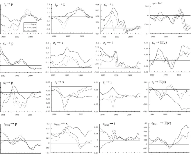
Figure 1 shows the time-varying impulse responses for TVP-VAR with stochastic volatility
using the …rst speci…cation: CPI in‡ation, the GDP gap, the call rate, and the
household-sector expectations for livelihood.7 The time-varying impulse responses at one-, two-, and
three-year horizons are shown over time, indicating structural changes in macroeconomic dynamics, including the private-sector expectations indicator. The columns correspond to
the impulse responses of variables to shocks from CPI in‡ation, the GDP gap, the call rate,
and the household-sector expectations for livelihood, respectively. The rows correspond to
the impulse responses of CPI in‡ation, the GDP gap, the call rate, and the household-sector
expectations for livelihood to shocks, respectively.
Several points should be noted regarding changes in the impulse responses over time.
First, the impulse responses of CPI in‡ation to the GDP gap shock weakened from the
second half of the 1990s when the call rate was lowered to 0.5 percent (the second row in the …rst column). Especially after the introduction of the ZIRP in 1999, the impulse
responses declined further to marginally negative. Similarly, the impulse responses of the
GDP gap to the CPI in‡ation shock continued to decline from 1999 and more recently
remained around zero (the …rst row in the second column).
Second, the impulse responses of the call rate to both the GDP gap and the CPI in‡ation
shocks remained at almost zero from 1999 (the …rst or second row in the third column).
That re‡ected the fact that additional room for cutting the call rate was exhausted in
facing the zero lower bound constraint of short-term nominal interest rates.8
7
We assume two lags for each variable, and the identi…cation ordering of CPI in‡ation, the GDP gap, the call rate, and the household-sector expectations for livelihood. We give a shock with the same-size, the average of one standard deviation of shocks for the whole sample period, in producing impulse responses.
Third, the impulse responses of both the GDP gap and CPI in‡ation to the call rate
shock were weakened from 1999, especially at the longer horizon, such as two or three
years (the third row and …rst or second column).9 that suggests that changes in interest
rates were unlikely to in‡uence prices and economic activity in the longer term under zero interest rate conditions.
Fourth, by contrast, the impulse responses of the household-sector expectations for
livelihood became signi…cant from 1999. The impulse responses to the CPI in‡ation and
the GDP gap shocks became negative and positive, respectively (the …rst or second row in
the fourth column). The impulse responses to the call rate shock became highly negative
at a one-year horizon, even though those at the two- and three-year horizons remained
close to zero (the third row in the fourth column). In addition, the impulse responses of
the household-sector expectations for livelihood to its own shock increased rapidly from 1999 (the fourth row in the fourth column). Those observations suggest the possibility that
dynamics in household-sector expectations formation were ampli…ed from 1999.
3.2 Business-sector activity and expectations
We next carry out a similar empirical exercise by using the expectations indicator for the
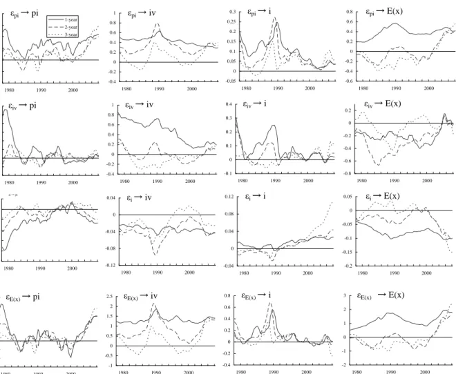
business sector. Figure 2 shows the time-varying impulse responses for TVP-VAR with
stochastic volatility using the second speci…cation: CGPI in‡ation, the investment gap,
the call rate, and the business-sector expectations for business conditions.10 We focus
particularly on the investment behavior of the business sector. Compared to consumption with smooth dynamics, investment is more responsive to economic conditions, which plays a
major role in business cycles. Thus, the monetary policy e¤ect is more sensitively re‡ected.
We see results similar to the …rst speci…cation. The interactions between the investment
the second half of the 1990s. That suggests that the assumption of stochastic volatility in disturbances contributes a great deal to improving the estimation precision in an extremely low interest rate environment.
9The call rate shock includes the e¤ect of the commitment policy in particular after 1999. Thus, both
the policy rate change and the commitment to future monetary policy easing generate impulse responses.
1 0We assume two lags for each variable, and the identi…cation ordering of CGPI in‡ation, the investment
gap and CGPI in‡ation were weakened under a very low interest rate environment (the …rst
row in the second column, and the second row in the …rst column). The impulse responses
of the call rate to both the investment gap and the CGPI in‡ation shocks became virtually
zero from 1999 (the …rst or second row in the third column). The impulse responses of both the investment gap and CGPI in‡ation to the call rate shock declined from 1999 (the
third row in the …rst or second column). However, the policy commitment induced larger
responses of the business-sector expectations for business conditions to the call rate shock
(the third row in the fourth column). The shock in expectations seems to have produced
more ampli…ed dynamics in business-sector expectations formation from 1999 (the fourth
row in the fourth column).
3.3 Interaction between expectations indicators
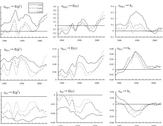
To clarify the e¤ect of policy commitment on private-sector expectations, we estimate a TVP-VAR with stochastic volatility using the third speci…cation: the household-sector
expectations for general prices, the household-sector expectations for livelihood, and the
long-term interest rate.11 Figure 3 shows the time-varying impulse responses.
We note two points. First, the impulse responses of the household-sector expectations
for general prices to the shock from the household-sector expectations for livelihoods
be-came stronger from 1999, especially at two- and three-year horizons, when the BOJ adopted
the policy commitment (the second row in the …rst column). The impulse responses of the
household-sector expectations for livelihoods to the shock from the household-sector ex-pectations for general prices also became stronger from 1999 (the …rst row in the second
column). Those two panels imply that the policy commitment induced a positive
interac-tion between prices and livelihood expectainterac-tions in the household sector. In addiinterac-tion, the
impulse responses of both the household-sector expectations for livelihoods and for general
prices to their own shocks strengthened from 1999, indicating the possibility that the policy
commitment ampli…ed dynamics in household-sector expectations formation (the …rst row
1 1
We assume two lags for each variable, and the identi…cation ordering of the household-sector expecta-tions for general prices, the household-sector expectaexpecta-tions for livelihood, and the long-term interest rate.
in the …rst column for price expectations and the second row in the second column for
livelihood expectations).
Second, the impulse responses of the household-sector expectations for livelihood to the
long-term interest rate shock increased from 1999 (the third row in the second column). The impulse responses of the household-sector expectations for general prices to the
long-term interest rate shock also showed a similar but weaker result (the third row in the …rst
column).
We conclude that the two episodes of the policy commitment by the BOJ did not
signi…cantly change dynamics within macroeconomic variables, such as output, investment,
prices, and interest rates, even under an extremely low interest rate environment from
1995. Nevertheless, we …nd some empirical evidence that the policy commitment was more
likely to stimulate private-sector expectations when extending our empirical framework to incorporate private-sector expectations indicators. We should add that such stimulative
e¤ects on private-sector expectations, however, were not transmitted to economic activity,
thus failing to completely reverse de‡ationary expectations in the economy.
4
Conclusions
Woodford (2005) emphasizes that a declaration of a monetary policy rule as the clearest
communication policy enables a central bank to control the real variables as well as the
agents’future expectations even under a liquidity trap. In this paper, we investigated the
e¤ect of the BOJ’s policy commitment under zero interest rates using macro data. We
found empirical results suggesting that the BOJ’s policy commitment on the future course
of short-term interest rates, even with a small reduction in current policy interest rates,
succeeded in changing private-sector expectations in a positive direction in the household and business sectors. Such a commitment e¤ect, nevertheless, did not spread throughout
the overall economy. That suggests that the monetary policy commitment was not a
cure-all measure for structural impediments that induced downward shifts in the trend growth
path.
per-sistent adverse shock due to insu¢ cient structural adjustments as a consequence of the
bursting of the asset price bubble in the early 1990s, as discussed in Okina and Shiratsuka
(2004b). What the BOJ faced during the period of the ZIRP and QEP was not a standard
stabilization policy around a stable trend growth path, but a policy management in an environment characterized by hampered sustained growth. However, in practice, it is not
easy to distinguish the nature of a shock on a real-time basis, given the limited knowledge
about economic structures.
References
[1] Eggertsson, Gauti, and Michael Woodford, “The Zero Bound on Interest Rates and
Optimal Monetary Policy,”Brookings Papers on Economic Activity, 1, 2003, pp. 139–
211.
[2] Fujiki, Hiroshi, Kunio Okina, and Shigenori Shiratsuka, “Monetary Policy under Zero
Interest Rate: Viewpoints of Central Bank Economists,”Monetary and Economic
Studies, Institute for Monetary and Economic Studies, Bank of Japan, 19 (1), 2001,
pp. 89-130.
[3] ______, and Shigenori Shiratsuka, “Policy Duration E¤ect under the Zero Interest
Rate Policy in 1999-2000: Evidence from Japan’s Money Market Data,”Monetary
and Economic Studies, Institute for Monetary and Economic Studies, Bank of Japan,
20 (1), 2002, pp. 1-31.
[4] Hara, Naoko, Naohisa Hirakata, Yusuke Inomata, Satoshi Ito, Takuji Kawamoto,
Takushi Kurozumi, Makoto Minegishi, and Izumi Takagawa, “The New Estimates
of Output Gap and Potential Growth Rate,”Bank of Japan Review, Bank of Japan,
No. E-3, 2006.
[5] Jung, Taehun, Yuki Teranishi, and Tsutomu Watanabe, “Optimal Monetary Policy at
the Zero-Interest-Rate Bound,”Journal of Money, Credit and Banking, 37 (5), 2005,
[6] Kimura, Takeshi, Hiroshi Kobayashi, Jun Muranaga, and Hiroshi Ugai, “The E¤ect
of the Increase in the Monetary Base of Japan’s Economy at Zero Interest Rates:
An Empirical Analysis,” in Monetary Policy in a Changing Environment, Bank for
International Settlements Conference Series, 19, 2003, pp. 276–312.
[7] Levin, Andrew, David Lopez-Salido, Edward Nelson, and Tack Yun, “Limitations
on the E¤ectiveness of Forward Guidance at the Zero Lower Bound,”International
Journal of Central Banking, 6 (1), 2010, pp. 143–189.
[8] Nakajima, Jouchi, “Time-varying Parameter Structural Vector Autoregression: A
Sur-vey of Methodology and Empirical Analyses,” manuscript, 2009.
[9] Oda, Nobuyuki, and Kazuo Ueda, “The E¤ect of the Bank of Japan’s Zero Interest
Rate Commitment and Quantitative Monetary Easing on the Yield Curve: A
Macro-Finance Approach,”Bank of Japan Working Paper, Bank of Japan, No. E-6, 2005.
[10] Okina, Kunio, and Shigenori Shiratsuka, “Policy Commitment and Expectation
For-mation: Japan’s Experience under Zero Interest Rates,”North American Journal of
Economics and Finance, 15 (1), 2004a, pp. 75–100.
[11] ______, and ______, “Asset Price Fluctuations, Structural Adjustments, and
Sustained Economic Growth: Lessons from Japan’s Experience since the Late 1980s,”
Monetary and Economic Studies, Institute for Monetary and Economic Studies, Bank
of Japan, 22 (S-1), 2004b, pp. 143–167.
[12] Primiceri, E. Giorgio, “Time Varying Structural Vector Autoregressions and Monetary
Policy,”Review of Economic Studies, 72, 2005, pp. 821–852.
[13] Ugai, Hiroshi, “E¤ects of the Quantitative Easing Policy: A Survey of Empirical Analyses,”Monetary and Economic Studies, Institute for Monetary and Economic
[14] Woodford, Michael, “Central-bank Communication and Policy E¤ectiveness,” in
In-‡ation Targeting: Implementation, Communication and E¤ ectiveness, Sveriges
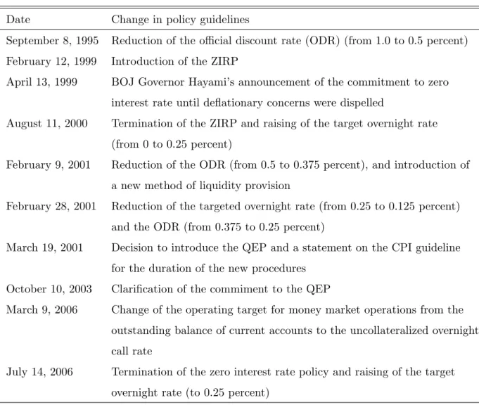
Table 1: Policy Events
Date Change in policy guidelines
September 8, 1995 Reduction of the o¢ cial discount rate (ODR) (from 1.0 to 0.5 percent) February 12, 1999 Introduction of the ZIRP
April 13, 1999 BOJ Governor Hayami’s announcement of the commitment to zero interest rate until de‡ationary concerns were dispelled
August 11, 2000 Termination of the ZIRP and raising of the target overnight rate (from 0 to 0.25 percent)
February 9, 2001 Reduction of the ODR (from 0.5 to 0.375 percent), and introduction of a new method of liquidity provision
February 28, 2001 Reduction of the targeted overnight rate (from 0.25 to 0.125 percent) and the ODR (from 0.375 to 0.25 percent)
March 19, 2001 Decision to introduce the QEP and a statement on the CPI guideline for the duration of the new procedures
October 10, 2003 Clari…cation of the commiment to the QEP
March 9, 2006 Change of the operating target for money market operations from the outstanding balance of current accounts to the uncollateralized overnight call rate
July 14, 2006 Termination of the zero interest rate policy and raising of the target overnight rate (to 0.25 percent)
0 0.05 0.1 0.15 0.2 0.25 0.3 1980 1990 2000 1-year 2-year 3-year εp→ p -0.2 -0.1 0 0.1 0.2 0.3 0.4 0.5 0.6 1980 1990 2000 εx→ p -0.4 -0.3 -0.2 -0.1 0 0.1 0.2 0.3 1980 1990 2000 εp→ x -0.04 0 0.04 0.08 0.12 0.16 1980 1990 2000 εp→ i -0.1 -0.05 0 0.05 1980 1990 2000 εp→ E(c) -0.1 0 0.1 0.2 0.3 0.4 0.5 1980 1990 2000 εx→ x -0.05 0 0.05 0.1 0.15 0.2 0.25 0.3 1980 1990 2000 εx→ i -0.08 -0.04 0 0.04 0.08 0.12 1980 1990 2000 εx→ E(c) -0.04 -0.03 -0.02 -0.01 0 0.01 0.02 1980 1990 2000 εi→ p -0.12 -0.1 -0.08 -0.06 -0.04 -0.02 0 0.02 1980 1990 2000 εi→ x -0.06 -0.03 0 0.03 0.06 1980 1990 2000 εi→ i -0.03 -0.02 -0.01 0 0.01 1980 1990 2000 εi→ E(c) -0.15 -0.1 -0.05 0 0.05 0.1 0.15 0.2 1980 1990 2000 εE(c)→ p -0.1 -0.05 0 0.05 0.1 0.15 0.2 1980 1990 2000 εE(c)→ x -0.08 -0.04 0 0.04 0.08 1980 1990 2000 εE(c)→ i -0.04 -0.02 0 0.02 0.04 0.06 0.08 0.1 1980 1990 2000 εE(c) → E(c)
Figure 1: Impulse Responses for the Household Sector
Note: p: CPI in‡ation, x: GDP gap, i: call rate, E(c): household-sector expectations for livelihood.
-0.1 -0.05 0 0.05 0.1 0.15 0.2 1980 1990 2000 1-year 2-year 3-year εpi→ pi -0.1 -0.05 0 0.05 0.1 0.15 0.2 0.25 0.3 1980 1990 2000 εiv→ pi -0.4 -0.2 0 0.2 0.4 0.6 0.8 1 1980 1990 2000 εpi→ iv -0.05 0 0.05 0.1 0.15 0.2 0.25 0.3 1980 1990 2000 εpi→ i -0.6 -0.4 -0.2 0 0.2 0.4 0.6 0.8 1980 1990 2000 εpi→ E(x) -0.4 -0.2 0 0.2 0.4 0.6 0.8 1 1980 1990 2000 εiv→ iv -0.1 0 0.1 0.2 0.3 0.4 1980 1990 2000 εiv→ i -0.8 -0.6 -0.4 -0.2 0 0.2 1980 1990 2000 εiv→ E(x) -0.05 -0.04 -0.03 -0.02 -0.01 0 0.01 1980 1990 2000 εi→ pi -0.12 -0.08 -0.04 0 0.04 1980 1990 2000 εi→ iv -0.04 0 0.04 0.08 0.12 1980 1990 2000 εi→ i -0.2 -0.15 -0.1 -0.05 0 0.05 1980 1990 2000 εi→ E(x) -0.3 -0.2 -0.1 0 0.1 0.2 0.3 0.4 0.5 1980 1990 2000 εE(x)→ pi -1 -0.5 0 0.5 1 1.5 2 2.5 1980 1990 2000 εE(x)→ iv -0.4 -0.2 0 0.2 0.4 0.6 0.8 1980 1990 2000 εE(x)→ i -2 -1 0 1 2 3 1980 1990 2000 εE(x) → E(x)
Figure 2: Impulse Responses for the Business Sector
Note:pi: CGPI in‡ation,iv: investment gap, i: call rate,E(x): business-sector expectations for business conditions. "a !brefers to the impulse response ofbto a positive shock ofa.
-0.2 0 0.2 0.4 0.6 0.8 1980 1990 2000 1-year 2-year 3-year εE(pc)→ E(pc) 0 0.04 0.08 0.12 0.16 1980 1990 2000 εE(c)→ E(c) -0.3 -0.2 -0.1 0 0.1 0.2 0.3 0.4 0.5 1980 1990 2000 εE(pc)→ E(c) -0.1 0 0.1 0.2 0.3 0.4 1980 1990 2000 εE(pc)→ b5 0 0.05 0.1 0.15 0.2 0.25 1980 1990 2000 εE(c)→ E(pc) -0.04 -0.02 0 0.02 0.04 0.06 0.08 1980 1990 2000 εE(c)→ b5 -0.14 -0.12 -0.1 -0.08 -0.06 -0.04 -0.02 0 0.02 1980 1990 2000 εb5→ E(pc) -0.09 -0.06 -0.03 0 1980 1990 2000 εb5→ E(c) -0.06 -0.04 -0.02 0 0.02 0.04 1980 1990 2000 εb5→ b5
Figure 3: Impulse Responses for Expectations Indicators
Note: E(pc): household-sector expectations for general prices, E(c): household-sector expectations for livelihood,b5: long-term interest rate. "a !brefers to the impulse response ofbto a positive shock ofa.