Full Terms & Conditions of access and use can be found at
http://www.tandfonline.com/action/journalInformation?journalCode=tgsi20
Download by: [79.110.203.215] Date: 27 October 2017, At: 07:30
Geo-spatial Information Science
ISSN: 1009-5020 (Print) 1993-5153 (Online) Journal homepage: http://www.tandfonline.com/loi/tgsi20
Repurposing a deep learning network to filter and
classify volunteered photographs for land cover
and land use characterization
Lukasz Tracewski, Lucy Bastin & Cidalia C. Fonte
To cite this article: Lukasz Tracewski, Lucy Bastin & Cidalia C. Fonte (2017) Repurposing
a deep learning network to filter and classify volunteered photographs for land cover and land use characterization, Geo-spatial Information Science, 20:3, 252-268, DOI: 10.1080/10095020.2017.1373955
To link to this article: http://dx.doi.org/10.1080/10095020.2017.1373955
© 2017 Wuhan University. Published by Taylor & Francis Group
Published online: 18 Sep 2017.
Submit your article to this journal
Article views: 137
View related articles
https://doi.org/10.1080/10095020.2017.1373955
KEYWORDS land cover; land use; volunteered geographic information (VGi); photograph; convolutional neural network; machine learning
ARTICLE HISTORY received 8 april 2017 accepted 19 June 2017
© 2017 Wuhan University. published by taylor & francis Group.
this is an open access article distributed under the terms of the creative commons attribution license (http://creativecommons.org/licenses/by/4.0/), which permits unrestricted use, distribution, and reproduction in any medium, provided the original work is properly cited.
CONTACT lucy Bastin [email protected]
Repurposing a deep learning network to filter and classify volunteered
photographs for land cover and land use characterization
Lukasz Tracewskia , Lucy Bastina and Cidalia C. Fonteb
aschool of engineering and applied science, aston University, Birmingham, UK; bDepartment of mathematics, inesc coimbra, University of
coimbra, coimbra, portugal
ABSTRACT
This paper extends recent research into the usefulness of volunteered photos for land cover extraction, and investigates whether this usefulness can be automatically assessed by an easily accessible, off-the-shelf neural network pre-trained on a variety of scene characteristics. Geo-tagged photographs are sometimes presented to volunteers as part of a game which requires them to extract relevant facts about land use. The challenge is to select the most relevant photographs in order to most efficiently extract the useful information while maintaining the engagement and interests of volunteers. By repurposing an existing network which had been trained on an extensive library of potentially relevant features, we can quickly carry out initial assessments of the general value of this approach, pick out especially salient features, and identify focus areas for future neural network training and development. We compare two approaches to extract land cover information from the network: a simple post hoc weighting approach accessible to non-technical audiences and a more complex decision tree approach that involves training on domain-specific features of interest. Both approaches had reasonable success in characterizing human influence within a scene when identifying the land use types (as classified by Urban Atlas) present within a buffer around the photograph’s location. This work identifies important limitations and opportunities for using volunteered photographs as follows: (1) the false precision of a photograph’s location is less useful for identifying on-the-spot land cover than the information it can give on neighbouring combinations of land cover; (2) ground-acquired photographs, interpreted by a neural network, can supplement plan view imagery by identifying features which will never be discernible from above; (3) when dealing with contexts where there are very few exemplars of particular classes, an independent a posteriori weighting of existing scene attributes and categories can buffer against over-specificity.
1. Introduction
In recent years, there has been an explosion in the popularity and prevalence of spatial data generation by citizens, through active collection initiatives such as OpenStreetMap, games and citizen science projects which tackle a wide range of topics, such as invasive spe-cies (Delaney et al. 2008), disaster response (Goodchild and Glennon 2010), cropland expansion (Fritz et al. 2012) and election violence (Meier 2008). This prolifer-ation of data co-creprolifer-ation has been facilitated by the avail-ability of cheaper sensors and GPS in smartphones. Web 2.0 technologies facilitate sharing, co-editing and online quality assessment of the generated information. Hand in hand with this active data generation is a rapid increase in the volume of voluntarily published resources, such as photos and reviews which are associated with some sort of locational information. Many terms have been coined to describe these types of data generated by the public but the term we will use to describe this particular
mix of actively and passively published spatially refer-enced data is volunteered geographic information (VGI) (Goodchild 2007). One of the phenomena that may be mapped using such VGI sources (potentially in combi-nation with more authoritative data) is land cover/land use. Geo-tagged photographs published to libraries, such as Flickr and Panoramio, are being increasingly investigated as potential sources of information in this context (Antoniou et al. 2016). If salient features can be identified and the position of the photographer is relatively certain, a subset of such photos may be useful for verifying and validating land cover/land use maps, and identifying changes in the landscape such as dis-turbance and vegetation change. In some cases, photo-graphs may be presented to volunteers as part of a game (e.g. MissingMaps), which requires gamers to interpret relatively complex photographs to extract relevant facts about phenomena such as disturbance, agricultural practices or settlements (Fritz et al. 2012). Thus far, the
OPEN ACCESS
primary source of imagery for such applications has been aerial or satellite photography (e.g. detailed imagery from DigitalGlobe is used in the Tomnod platform) which offers a plan view of the ground. However, there is a potential role for volunteered photographs taken for entirely different purposes and published in repositories (e.g. Flickr) to fill the gaps, where no aerial imagery is available and to add significant value in terms of iden-tifying key landscape features. The key challenge when exploiting such a vast and heterogeneous data source is to identify the most relevant and useful photographs from the deluge of available candidates, in order to most efficiently extract useful information while maintaining the engagement and interest of any volunteers assisting with classification. One option for automating this fil-tering process is to apply machine learning approaches such as deep learning to the content and metadata of the photographs, in combination with a user-defined set of priorities which define fitness for a particular purpose. The priorities of the original photographer submitting photos to Flickr will rarely align with those of a scientist trying to repurpose the image, so it is vital to identify the most salient images to avoid being swamped by irrele-vant information.
This paper extends recent research into the useful-ness of volunteered photos for land cover extraction, and investigates whether this usefulness can be auto-matically assessed in order to best focus citizen science efforts. We revisit a set of photos harvested from the web which were assessed for their usefulness by experts (Antoniou et al. 2016) and evaluates the degree to which the rule-based classification from the experts can be rep-licated by a neural network on the basis of the features identified in the photos. By repurposing an existing net-work which had been trained on an extensive library of potentially relevant features, we were able to carry out initial assessments of the general value of this approach, pick out features which were especially salient, and iden-tify focus areas for future neural network training and development for this specific purpose. This approach also allowed us to test methods accessible to a general audience without specialized development and coding expertise.
2. Related work
2.1. Land cover and land use mapping—the context
Land cover or land use mapping is usually performed through the classification of satellite imagery. A variety of nomenclatures can be used in Land cover and land use mapping, some corresponding to land cover data and some also including land use information, such as CORINE Land Cover (European Environmental Agency 2006) or the Global Monitoring for Environment and Security Urban Atlas (UA) (European Environmental
Agency 2012). The classification of land cover corre-sponds to the biophysical cover of the earth’s surface, while land use is associated with arrangements, activities and inputs humans undertake for related to a certain type of land cover. The identification of different types of land cover using satellite imagery is easier than the identification of land use, since the latter often does not correspond to characteristics easily identifiable in aerial or satellite imagery using just reflectance. For example, a region covered with grass may correspond to several types of land use, such as sport fields, public or private parks or natural grassland. The opposite can also hap-pen—a land use class, such as recreation areas, often includes several types of land cover.
Information about land use can be relatively easily provided by volunteers or be often easily identifiable in photographs taken at the earth’s surface. Therefore, information provided by volunteers may be valuable, either when they are asked to identify land use classes directly, such as when creating vector data correspond-ing to land use information in OpenStreetMap, or by using photographs taken by the citizens. In the second context, the volunteers do not provide the land use/cover classes directly, but provide the data from which it can be extracted. The use of different nomenclatures raises problems when several sources of land use/land cover data are to be compared or combined. This requires the establishment of a mapping between nomenclatures. Even though this mapping is not always easy, several harmonization mappings are available for different nomenclatures (Arnold et al. 2013; Fonte et al. 2017). 2.1.1. Volunteered photos—the context
A thorough summary of online photo repositories and their protocols can be found in Antoniou et al. (2016). Some (currently relatively small) repositories focus spe-cifically on land cover and land use; among these are the Degree Confluence Project and the Field Photo Library (Xiao et al. 2011). These data sources are well used for environmental modelling and validation (Foody and Boyd 2012; Iwao et al. 2006; Leinenkugel et al. 2014). These data can be assumed to be of interest for the pur-poses of this research. Therefore, we focus on expand-ing and supplementexpand-ing this resource by repurposexpand-ing and filtering public photographs from other domains, exploiting online repositories such as Flickr, Panoramio, Geograph and Instagram. The above-mentioned repos-itories host billions of photographs. These content and metadata is increasingly being analyzed to draw infer-ences about human social behaviour, tourism and the urban environment. The pool of photographs is rapidly expanding, with around 2 million public photographs a day being uploaded to Flickr (Franck 2016) and 58 million per day to Instagram (StatisticBrain 2016). Naturally, as alternative photo publishing platforms within a commercial market ecosystem, the repositories
differ in their focus and the dominant themes of the pic-tures published. A rough idea of these differences can be gained by investigating the optional text tags with which images are annotated. In terms of the images published which are shared publicly.
2.1.2. Flickr
Flickr leans towards the art and landscape side of pho-tography, with numerous comments and discussions centred on the techniques used to capture or process images: trending tags often include topics such as ‘depth of field’ and ‘exposure’. Because of this focus, many of the submitted photographs address landscapes: the all-time most popular image tags include ‘sunset’, ‘water’, ‘sky’, ‘nature’, and ‘tree’. While these themes would appear very relevant to the recognition of landscape features and land cover, it is important to remember that these landscapes are frequently long shots that give little infor-mation about the location of the photographer (i.e. the actual geotag) and may be substantially processed. 2.1.3. Panoramio
Panoramio has a fundamentally spatial focus, since it specifically aims to showcase images attached to specific locations. The acquisition of Panoramio by Google in 2007 enhanced this function by embedding Panoramio pictures directly into Google Earth and Google Maps. Photo volumes in Panoramio are more modest; an esti-mated 93 million photos have been uploaded to the Panorank repository, but images are frequently deleted as users replace them with better versions, so the current number is probably lower. Daily estimates are not reg-ularly monitored, but are estimated at between 20 and 40 thousand images per day; however, the frequency of geotagging is far higher than with Flickr photos. Tags, unsurprisingly, also frequently include concepts relevant to landscape features, such as ‘mountain(s)’, ‘nature’, ‘for-est’, ‘river’, and ‘urban’.
2.1.4. Geograph
The Geograph Project is an initiative designed to col-lect representative images across a number of sampling regions, namely, Britain and Ireland, Germany and the Channel Islands. The goal is for participants to collect at least one image for every square kilometer of these regions. Photographs tend to include architectural fea-tures or characteristic landscapes, and location and view direction are associated with the picture, since it is obligatory to report the position of the viewer and of the subject.
2.1.5. Instagram
As a social media platform, which is increasingly used for viral marketing by companies and celebrities, Instagram’s trending tags are (at the time of writing at least) dominated by terms, such as ‘cute’, ‘selfie’, ‘fashion’ and ‘best friends’. While various APIs are available for
consuming georeferenced Instagram feeds (for example, Esri’s GeoEvent connector) it was felt that for the pur-poses of this work, the streams of photos would require too much filtering, and so we confined the analysis to Flickr, Geograph and Panoramio. This also allowed us to evaluate our results against the work of Antoniou et al. (2016) by re-evaluating a set of data previously analyzed in their work.
2.2. Deep learning
Efficient filtering and classification of photographs to extract information on land use or land cover require a computer program to understand abstract concepts related to the interpretation of scene content. By using neural networks (Schmidhuber 2015) it is possible for software to learn these rules from a training set, with-out having to handcraft features (i.e. to characterize the elements of a scene in mathematical form) and pro-vide them as inputs to a model. Neural networks are used in contexts where it is necessary to derive a rela-tionship between variables, and where there are some observations of that relationship which can be used to train the network. A neural network is trained by prop-agating input data through layers of nodes to produce output values, which are then compared to the ‘truth’ to assess the goodness-of-fit. The desired output values may be continuous or discrete. Neural networks are most commonly used to assign categorical labels on the basis of continuous multivariate input data − for example, to recognize a text character from a variety of metrics derived from a pixelated image. Weightings in intermediate nodes are used to transform the input values to output, and these are iteratively adjusted to optimize the fit of the model. This process, known as ‘back-propagation’, allows the characteristics of a specific data set to be learnt. Unless the training data is extensive, with good representation of all the types of features to be distinguished, it runs a high risk of ‘over-fitting’, so that the model cannot reliably be applied to novel data. Over-represented classes in the training data can act as ‘attractors’ and significantly bias the accuracy of the final model. This is an important constraint in the context of VGI, which tends to be spatially patchy and biased towards particular themes.
The hidden layer is instantiated with values (most often random) which are later refined through back-propagation. The layer is called ‘hidden’, since it is difficult to provide an interpretation of the weights and what the network has learned.
Once there are three or more hidden layers in the neural network, we usually consider it deep—hence the term ‘deep learning’. Fully connecting all neurons of one layer with all neurons of the next layer can lead to very complex optimization problems. For example, if an image with resolution 1000 by 1000 pixels is submitted to the network with one pixel value on each input, it
(Fritz et al. 2015), the identification of invasive species in Hawaiian forests, the assessment of disturbance in and around protected areas (Bastin et al. 2013) or the recent ‘gamification’ of validation of the GlobeLand30 product (Brovelli et al. 2016). This ‘view-from-above’ has parallels with the classic remote sensing approach to landscape characterization, but instead of relying on spectral signatures or backscatter characteristics, land cover and land use types are identified by their char-acteristic shapes and patterns, easily picked out by the human eye.
Less frequently, photographs taken at ground level are used to record or verify land cover and land use maps, and in these cases many other factors come into play: for example, the focal length, orientation and viewpoint of a photograph, the accuracy of its locational information and its currency (many users of photo-sharing platforms upload scanned postcards or historic photos). Antoniou et al. (2016) analyzed the types of metadata that may be available associated to geo-tagged photographs, and which are available for Flickr, Panoramio and Geograph. Among these are orientation, date of upload and acqui-sition, focal length, tags, descriptions, titles and infor-mation about the photographer. The metadata required (mandatory and volunteered) varies according to the initiative and therefore, the metadata available for the photographs varies with their origin.
Many analyses which using volunteered photos use information other than the image itself: for example, parsing and using the associated tags to identify features of interest and delineating the areas (sometimes fuzzily defined) which users see as belonging to a particular named location (Gao et al. 2014; Li and Goodchild 2012) or see as attractive (Hu et al. 2015). On occasion, information about the user’s identity is used to map tra-jectories (Jankowski et al. 2010) and or identify “local-ness” in shared photos and tweets (Johnson et al. 2016). Antoniou et al. (2016) analyzed the availability of tags, descriptions and titles in a set of 1000 photographs from each of Flickr, Panoramio and Geograph in the London area (corresponding to a total of 3000 photographs). The content of the harvested resources was not analyzed in that study, but only their availability and the number of available tags and words (for the descriptions and titles). The results show that for Geograph, only 34% of the pho-tographs had tags, and this number increased to 70 and 79%, respectively, for Flickr and Panoramio, though the mean number of tags was smaller for Panoramio than for Flickr. This shows that the use of tags to identify the content of the photographs may leave out of the analysis a large number of photographs which could be useful to extract information. Therefore, methods that allow the analysis of the photographs themselves, instead of just the associated metadata, are useful.
Visual feature matching may be performed to identify landmarks (Kisilevich et al. 2010) or group photographs (Kennedy et al. 2007), but identification of land cover or effectively means 106 values on input. Connecting the
input layer with a hidden layer of the same size gener-ates 1012 parameters to optimize. Adding more layers
not only will lead gargantuan complexity, but will also cause severe overfitting: the neural network will do an excellent job in handling the cases it was trained on, but very poorly on new data sets (Schmidhuber 2015; Srivastava et al. 2014).
Convolutional Neural Networks (CNNs) address these problems and offer significant improvements over previous approaches (Krizhevsky, Sutskever, and Hinton 2012). Their architecture takes into account the spatial structure present in images, and introduces between the layers of the network an additional series of ‘convolu-tional layers’, each focusing on a particular region of the image. In order to further improve efficiency, parame-ters are shared across the network. Thus, the detection of a particular type of feature (to take a simple exam-ple, a vertical edge), once ‘learnt’ in one region, can be detected wherever it occurs in the image. As with the visual cortex of many animals, there is some overlap between the regions into which the image is divided. This region-based approach still makes local connec-tivity between neurons much easier to maintain, and allows the network to learn increasingly higher levels of abstractions. This makes the layers much easier to train, while having good grounds in computer vision and exploiting the phenomenon of spatial autocor-relation in imagery: distant regions within images are rarely semantically connected, but salient feature types, such as the aforementioned vertical edges, can occur anywhere in an unfamiliar image. A remarkable feature of this class of machine learning algorithms is the ability to generalize well and significantly outper-form other approaches when it comes to dealing with abstract problems (Krizhevsky, Sutskever, and Hinton 2012; Schmidhuber 2015). Teaching the neural network to recognize a feature such as forest simply requires that the algorithm is shown sufficient number of photographs depicting forest, without having to explicitly define what ‘forest’ is. What constitutes ‘enough’ depends strongly on the complexity and variety of what the program tries to learn, but will require at least a few hundred labelled images per class. The requirement for a large number of training examples, as well as the computational power required for processing, can present a significant chal-lenge, and for this reason, we took advantage of a ready-made model, which is further described below.
2.3. Identifying land cover from photos
In recent years a number of interesting initiatives have involved volunteers in identifying land cover and land use from images. In some cases, these are images taken from space or from the air, for example, the Geowiki cropland mapping initiative which asked volunteers to solve conflicts in widely used classified land cover maps
The CNN used in this study, Places205-AlexNet (Zhou et al. 2014), was trained by its authors on almost 2.5 million photographs, this allowed it to achieve 50% accuracy on identifying 205 “scene categories” (this term is explained in detail below). It should be noted that the choice was made purely on the wide availability of the pre-trained models for this neural network architecture and could be replaced with more accurate models. Training of the algorithm is an iter-ative process that usually a requires very large num-ber of passes over the complete data set, making it a computationally expensive process which necessitates a huge set of labelled samples for training, analogous to the ‘ground truth’ of remote sensing classifications. In addition to this significant investment of resources, the creation of such a model requires expertise in computer vision and machine learning. For that rea-son, a number of studies, including this one, focus on retrofitting existing models, rather than building models from scratch.
Automated classification of photographs is highly rel-evant for those applications which involve volunteers in games or campaigns to identify interesting features from photos, since many photos are irrelevant, and simply presenting all available material runs the risk of boring volunteers and causing them to disengage. Ideally, we would like to filter photos in order to:
(1) Identify photos which are irrelevant or non-use-ful, and discard them;
(2) Identify images from which land cover/land use can be quickly and reliably identified (for exam-ple some types of built environment), harvest the labels and discard the photos from further analysis;
(3) Identify candidate land covers in the vicinity of remaining images for verification by volunteers (4) Identify challenging and interesting photos
that a user may enjoy deconstructing to extract more information than a machine can do. The developed methodologies were applied to two study areas; one is the region used in Antoniou et al. (2016) that is situated in an urban area of London, UK and the other is located northwest of Paris, France, in a region which covers part of central Paris (as far South as Notre Dame) but also extends Northwards to a region with low-density urban areas and predominance of agri-culture and forest. Since the London area was predomi-nated by built environment and man-made features, the Paris region was selected in order to extend the classi-fication challenge to a wider variety of land covers and land uses.
Within this study we aimed to assess how far we could achieve several distinct goals, as follows:
(1) Automating the identification of photographs which are useful for land cover classification. human disturbance from the photos themselves is, at the
time of writing, less frequently researched. Deep learn-ing approaches are ever more widely used to generate maps from images: for example, the Facebook initia-tive to map settlement configurations across 20 coun-tries using 14.6 billion DigitalGlobe images at 50 cm resolution (350 TB data), combined with census data (Gros and Tiecke 2016) or the work by Castelluccio et al. (2015) to delineate land use types from the charac-teristic features which may be seen in detailed imagery. Albert, Kaur, and Gonzalez (2017) have also recently successfully classified typologies of city neighbourhoods using deep learning approaches combined with satellite imagery from Google Maps.
However, the above initiatives rely on the classic plan that delineates features from above, leaving scope for extra information to be gained from images acquired at the ground level. The closest work to what is addressed in this paper is that from Leung and Newsam (2015) who derived a classification of developed vs. undevel-oped land for the UK, using photographs harvested from Flickr and Geograph, and (Zhu and Newsam 2015) − a campus mapping exercise which derived eight land use types from volunteered photographs in combination with a shapefile representing the zones on site.
In the study by Leung and Newsam (2015), the chal-lenge of providing enough labelled images to train the machine learning algorithm was resolved by inferring the label through natural language processing from a description provided by the user. As the authors note, user-supplied text for an individual image is often not sufficient to assign it to a class, and so 1 × 1 km tiles were used to group photographs, in order to model topics efficiently. The authors use handcrafted features, namely colour histogram, edge histogram and gist descriptors, to train their model for scene recognition. Zhu and Newsam (2015), on the other hand, took the same approach to classification by using an off-the-shelf model, AlexNet (Krizhevsky, Sutskever, and Hinton 2012).
3. Specific approach for this study
In this work, we aimed to assess how far an off-the-shelf model which had been trained on a variety of potentially useful features could be adapted for our needs. The goal is to derive useful labels for a land cover or land use context without the need for an extensive gathering of ‘ground truth’, development of significant amounts of code, or heavy computational training of the network. An equally important goal is to assess and evaluate the limitations of this ‘off-the-shelf’ approach, and to try to characterize those contexts and photograph types where it is less reliable. In this way, we aim to derive some guidelines for best practice in the use of pre-trained models for specific use cases in the exploitation of volunteered photographs.
3.1. Selection and setting up of algorithm and model
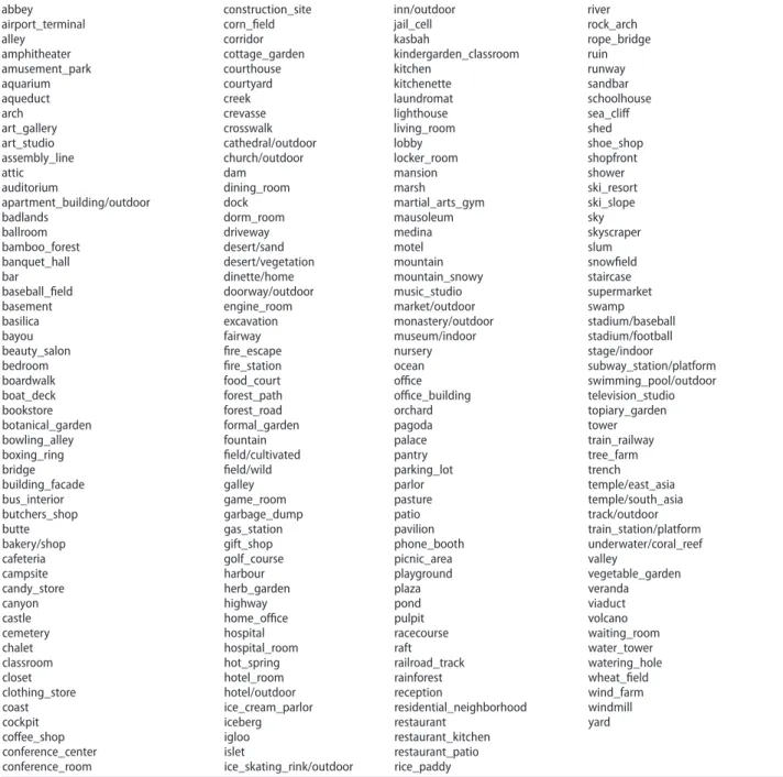
The Places205-AlexNet neural network (Zhou et al. 2014) has nine layers: an input layer, seven hidden lay-ers and an output layer. The output layer consists of 205 scene categories, such as abbey, bedroom or mountain; a full list is provided in Table 1. The model outputs a value for each category, indicating the probability that a photo belongs to a certain class. This capacity is the result of training on MIT’s Places database (http://places.csail. mit.edu/), a set of 2.5 million images, each labelled with a scene category. A novel image classified with this pre-trained network will usually belong to many categories, with varying scores. The last hidden layer of the neural network also provides valuable information about the photo content: a set of 4096 values that, in combination, form a ‘signature’ of the image. They represent high-level (2) Extracting any information which can be
immediately derived about land cover/land use. (3) Relating the neural network outputs to an exist-ing land cover classification, to assess how far accepted classes can be identified from image features.
We drew on past research by Antoniou et al. (2016) and specifically aimed to replicate their rule-based clas-sification of photograph usefulness with an off-the-shelf combination of tools and a simple allocation of weights to tags which could be performed by a domain expert with no particular computational experience. The goal was to achieve a comparable stratification of images with much less investment of expert time, since the original classification of usefulness involved 7 experts each classifying 3 thousand photographs − a slow and tedious task.
Table 1. scene categories from the places205 project (Zhou et al. 2014).
abbey construction_site inn/outdoor river
airport_terminal corn_field jail_cell rock_arch
alley corridor kasbah rope_bridge
amphitheater cottage_garden kindergarden_classroom ruin
amusement_park courthouse kitchen runway
aquarium courtyard kitchenette sandbar
aqueduct creek laundromat schoolhouse
arch crevasse lighthouse sea_cliff
art_gallery crosswalk living_room shed
art_studio cathedral/outdoor lobby shoe_shop
assembly_line church/outdoor locker_room shopfront
attic dam mansion shower
auditorium dining_room marsh ski_resort
apartment_building/outdoor dock martial_arts_gym ski_slope
badlands dorm_room mausoleum sky
ballroom driveway medina skyscraper
bamboo_forest desert/sand motel slum
banquet_hall desert/vegetation mountain snowfield
bar dinette/home mountain_snowy staircase
baseball_field doorway/outdoor music_studio supermarket
basement engine_room market/outdoor swamp
basilica excavation monastery/outdoor stadium/baseball
bayou fairway museum/indoor stadium/football
beauty_salon fire_escape nursery stage/indoor
bedroom fire_station ocean subway_station/platform
boardwalk food_court office swimming_pool/outdoor
boat_deck forest_path office_building television_studio
bookstore forest_road orchard topiary_garden
botanical_garden formal_garden pagoda tower
bowling_alley fountain palace train_railway
boxing_ring field/cultivated pantry tree_farm
bridge field/wild parking_lot trench
building_facade galley parlor temple/east_asia
bus_interior game_room pasture temple/south_asia
butchers_shop garbage_dump patio track/outdoor
butte gas_station pavilion train_station/platform
bakery/shop gift_shop phone_booth underwater/coral_reef
cafeteria golf_course picnic_area valley
campsite harbour playground vegetable_garden
candy_store herb_garden plaza veranda
canyon highway pond viaduct
castle home_office pulpit volcano
cemetery hospital racecourse waiting_room
chalet hospital_room raft water_tower
classroom hot_spring railroad_track watering_hole
closet hotel_room rainforest wheat_field
clothing_store hotel/outdoor reception wind_farm
coast ice_cream_parlor residential_neighborhood windmill
cockpit iceberg restaurant yard
coffee_shop igloo restaurant_kitchen
conference_center islet restaurant_patio
conference_room ice_skating_rink/outdoor rice_paddy
(1) It is simple to apply, requiring only some invest-ment of time by one or more experts and some simple post-processing in a spreadsheet; (2) In theory, it should be proof against overfitting,
since the weights are assigned independently of any image training set;
(3) It should allow land covers which are rare in the training set to be adequately identified, since a user has independently flagged the tags which they consider to be indicative of those land covers.
(4) It allows derivation of a score for all images in the set, unlike a training/validation approach which requires a portion of the data to be set aside.
The more technical approach (referred to as decision tree [DT]) was based on supervised machine learning and involved building and training decision trees on the results from the original classification—an approach which requires little computational resources in com-parison to original network training, but one that still calls for specific expertise. Whereas in the UW approach we orchestrate rules ourselves, in the DT we allow the computer to find an optimal set for us. For the specific algorithm, we selected XGBoost (Chen and Guestrin 2016), an open-source software library that provides a distributed tree boosting framework. By using an ensem-ble of weak prediction models, it can capture general rules governing the system, without having to explicitly define the relationships between or the importance of parameters. The validity of the model was always tested with fivefold stratified cross-validation, while confusion matrices were generated with one of the folds. To avoid strong bias towards the training set, we used penalized classification and restricted the depth of the constructed decision trees (defined as the length of the longest path from a root to a leaf) to five.
For each of our goals, we build three models, one for each of the neural network outputs (scene catego-ries, scene attributes and numbers from the penulti-mate layer). We start by running a pre-trained model (in our case AlexNet) on images we would like to clas-sify and storing its output. The latter becomes input to DT and UW methods. DT, as any supervised method, also requires that we provide labels to the training data set. The advantage over neural network is that far fewer labelled examples are needed for the algorithm to achieve good results and also only a few hyperparameters are left to tune. Our source code repository (https://github.com/ RSPB/CitizenSensor) contains code for classification of images using pre-trained AlexNet model (in particular, file image_classifier.py) and an example of how to run the DT method (classification_example_with_xgb.py).
The contrasting approaches were applied to a series of goals (which define our output), as follows:
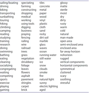
features of the image and it is from these values that scene categories are derived. A user can use this penulti-mate layer to build their own classifiers, and the authors of the Places205 network did just this, creating a set of 102 “scene attributes” which we have also used in our study. The scene attributes consist of classes like ‘ice’, ‘working’ or ‘trees’, with a full list to be found in Table 2. All of the mentioned values i.e. scene categories, scene attributes and the output of the last hidden layer, are used for classification in this work.
Some of the scene categories and attributes have clear relevance to land cover and land use: for example, ‘forest’, ‘rock arch’, and ‘ocean’. Others relate to materials and characteristics from which at least some inference may be made about the surroundings: for example, ‘shrub-bery’, ‘enclosed area’, and ‘concrete’. Many of the labels are related to human activities which might be carried out anywhere, or interpretations of a scene which do not allow any inferences to be drawn: for example, ‘reading’, ‘stressful’ or ‘business’.
In order to assess the value of our approach, we pro-cessed the output of the neural network in two differ-ent ways, in order to assess whether acceptable results could be achieved with a lightweight strategy available to relatively non-technical users. The simple approach (referred to as user-weighting [UW]) involved the allo-cation of binary weights (0 or 1), to each scene category and attribute, representing their relevance to particular categories of user interest (e.g. the land cover ‘agricul-ture’). Using this approach, all the scores for a photo-graph can be weighted and summed to achieve a score for each of the user-defined labels. The rationale for this approach is that:
Table 2. scene attributes from the places205 project (Zhou et al. 2014).
sailing/boating spectating tiles glossy driving farming concrete matte biking constructing metal sterile transporting shopping paper moist sunbathing medical wood dry touring working vinyl dirty hiking using tools plastic rusty climbing digging cloth warm camping business sand cold reading praying rocky natural studying fencing dirt soil man-made training railing marble open area research wire glass semi-enclosed area diving railroad waves enclosed area swimming trees ocean far-away horizon bathing grass running water nohorizon eating vegetation still water rugged
cleaning shrubbery ice vertical components socializing foliage snow horizontal components congregating leaves clouds symmetrical
waiting flowers smoke cluttered competing asphalt fire scary sports pavement natural light soothing exercise shingles sunny stressful playing carpet electric lighting
gaming brick aged
result as a match only if it was exact, i.e. the class found by the model was the same as the class labelled by the expert (in other words, the alternative class was not taken into account here).
(2) Goal 2: filtering photos by usefulness, based on per-ceived land cover
Antoniou et al. (2016) assessed a group of photo-graphs from the London area and asked a group of experts to look for nine different land covers within the photographs, as used within the Geo-Wiki project: tree cover, shrub cover, grassland/herbaceous, cropland, wet-land, artificial surfaces, bare rock/barren surface, snow/ ice and water. Based on the presence or absence of those land covers, the usefulness of the photographs for iden-tifying the classes was determined by experts, applying a set of rules that determined what the answer should be in case of doubts (Table 3).
In the UW approach, weights of 1 or 0 were assigned to associate each of the 205 scene categories and 102 scenes attributes with zero or more of the nine land cov-ers defined in the original study. For example, ‘rainforest’ is associated with the ‘forest’ land cover class, and ‘living room’indicates that a photo was taken within the built environment, but ‘praying’ cannot reliably be associated with any particular land cover or land use. This task was performed by one of the authors, and the resulting weights were multiplied by the image scores and aggre-gated to give a score for each of the aforementioned nine land covers, yielding 0 or more land cover labels for each photo. On the basis of these labels, thresholds and decision rules which mimicked Table 3 were applied to label each photo as ‘useful’, ‘maybe useful’; or ‘not useful’. Results for the London photos were validated against the original expert consensus (Antoniou et al. 2016) and for the Paris set, a subset of 965 photos were labelled by one of the authors as a validation set.
For the DT approach, the land cover identification step was skipped and the same validation labels were used for training in a fivefold cross-validation approach, to assess whether a model could learn the criteria for usefulness directly.
(1) Goal 1: identifying human impact in a landscape For this exercise, we defined five classes as follows: • bi = Built environment, indoors.
• b = Built environment, may be indoors or outdoors. • hf = Human feature (e.g. a bridge, railway line,
fountain, windmill) May be placed in a natural landscape.
• hl = Human land use (e.g. agriculture, gardens, golf course). Landscape may be vegetated but human influence is expected to affect a substantial area of the scene.
• n = Natural environment (and note that
u = unknown)
The reasoning is that these categories could be useful for studies of fragmentation, habitat disturbance, etc. Each scene category and attribute was given a weight of 1 if expected to be indicative of these classes. After summing all weighted scores, the ‘winning classes’ were determined using the following algorithm:
(1) Find classes with score above predefined threshold. The threshold is calculated as nth percentile of the highest scoring class. For our experiments, we used the 70th, 80th and 95th percentiles. The particular values were selected arbitrarily as means to tune the method. (2) If ‘bi’ class was found, ‘b’ was added, as ‘built
environment, indoors’ is a subset of ‘built environment’.
(3) If ‘b’ class was found, ‘hf’ was added, since buildings and other features characteristic of the urban environment are man-made features. One of the authors of this article labelled 965 pho-tographs with classes, while on 242 occasions assigning also an alternative class when it was not clear which class should be assigned to the photograph. In the UW method, we marked prediction as successful if any of the classes predicted by the algorithm was present as either the class or alternative class selected by the human expert. The DT approach was stricter: we considered a
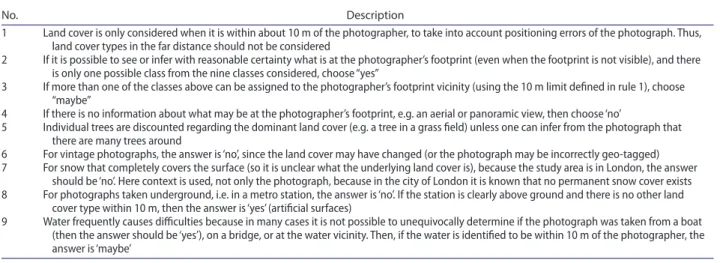
Table 3. rules used to assist in the classification of the photographs as useful, from antoniou et al. (2016).
No. Description
1 land cover is only considered when it is within about 10 m of the photographer, to take into account positioning errors of the photograph. thus, land cover types in the far distance should not be considered
2 if it is possible to see or infer with reasonable certainty what is at the photographer’s footprint (even when the footprint is not visible), and there is only one possible class from the nine classes considered, choose “yes”
3 if more than one of the classes above can be assigned to the photographer’s footprint vicinity (using the 10 m limit defined in rule 1), choose “maybe”
4 if there is no information about what may be at the photographer’s footprint, e.g. an aerial or panoramic view, then choose ‘no’
5 individual trees are discounted regarding the dominant land cover (e.g. a tree in a grass field) unless one can infer from the photograph that there are many trees around
6 for vintage photographs, the answer is ‘no’, since the land cover may have changed (or the photograph may be incorrectly geo-tagged) 7 for snow that completely covers the surface (so it is unclear what the underlying land cover is), because the study area is in london, the answer
should be ‘no’. Here context is used, not only the photograph, because in the city of london it is known that no permanent snow cover exists 8 for photographs taken underground, i.e. in a metro station, the answer is ‘no’. if the station is clearly above ground and there is no other land
cover type within 10 m, then the answer is ‘yes’ (artificial surfaces)
9 Water frequently causes difficulties because in many cases it is not possible to unequivocally determine if the photograph was taken from a boat (then the answer should be ‘yes’), on a bridge, or at the water vicinity. then, if the water is identified to be within 10 m of the photographer, the answer is ‘maybe’
goal aimed to determine if the classes associated with the photographs of the Paris region were correlated with the classes present in UA at the location of the photograph.
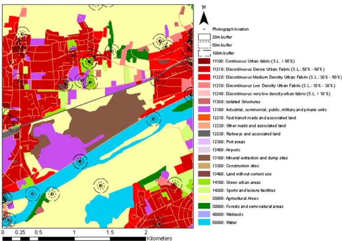
Figure 1 shows the locations of all the photographs harvested from the Paris study region, overlaid on the UA classification.
(4) Goal 4: identifying UA land cover classes in the sur-rounding area
In the process of discussing and evaluating the description of ‘usefulness’’ in the above section, it became even more apparent to us that the goal of identifying land cover at the georeferenced point from (3) Goal 3: identifying land cover as defined by UA
The European Environmental Agency’s Urban Atlas (https://cws-download.eea.europa.eu/local/ua2006/ Urban_Atlas_2006_mapping_guide_v2_final.pdf) is a high-resolution land use or land cover map of regions in Europe with more than 100 000 inhabitants. The created maps can be downloaded freely (https://www. eea.europa.eu/data-and-maps/data/urban-atlas). The created maps have a geometric scale of 1:10,000 and a minimum mapping unit of 0.25 ha for area features and 100 m for linear features. The nomenclature used in UA is organized into four levels of detail for the urban classes. Table 4 shows levels 2 and 4 of this nomen-clature, as these were the ones used in this study. This
Table 4. Ua classes of levels 2 and 4 (european Union, 2011, https://cws-download.eea.europa.eu/local/ua2006/Urban_at-las_2006_mapping_guide_v2_final.pdf).
Level 2 Level 4
Code Class name Code Class name
11 Urban fabric 1110 continuous urban fabric
1120 Discontinuous urban fabric 1121 Discontinuous dense urban fabric 1122 Discontinuous medium density urban fabric 1123 Discontinuous low-density urban fabric 1130 isolated structures
12 industrial, commercial, public, military, private, and transport units 1210 industrial, commercial, public, military and private units 1222 other roads and associated land
1223 railways and associated land 13 mine, dump and construction sites 1340 land without current use 14 artificial non-agricultural vegetated areas 1410 Green urban areas
1420 sports and leisure facilities
20 agricultural areas, semi-natural areas and wetlands 2000 agricultural areas, semi-natural areas and wetlands
30 forests 3000 forests
50 Water 5000 Water
Figure 1. Ua classes for the paris study region, with locations of all photographs overlaid. the abbreviation “s.l” in the legend refers to the proportion of sealed surface which helps to define that class.
which a photograph is taken is highly challenging. For example, a photographer may be standing on a bridge while photographing water, or on a boat while taking a photograph of land. It is vanishingly rare that a pho-tograph shared to a public image library will record a downward view of the location where the photographer is standing: rather, the images tend to represent tran-sects or cones of vision of varying length which record a variety of the features in the neighbourhood, and which could form a useful complement to the ‘plan-view’ aerial photography and satellite imagery used for classical land cover classifications. Without information on depth of field and orientation (such as that explicitly recorded for the European Commission’s LUCAS land cover survey and for the Degree Confluence project), it can be difficult to pin down the features located to exact locations. However, it is highly likely that future mobile phone development will make this easier, and that with sufficient volunteered photos, some useful triangula-tion could be done. In additriangula-tion, the mix of features within a view may itself be informative in identifying land uses which have characteristic mixes of features: for example, built areas which have some level of veg-etation. For this reason, we extended the above UA analysis to consider the land covers identified within 20, 50 and 100 m buffers around the reported location of the photograph. An example of these is shown in Figure 2.
Figure 2. example of 20, 50 and 100 m buffers around spots where photos were taken.
Table 5. frequency of Ua level 2 classes in the data set at the specific location of each photo (point) and in the area around it (buffer).
Class Point (%) buffer (%)20 m buffer (%)50 m buffer (%)100 m
11 28.3 27.9 28.4 26.9 12 37.6 41.3 38.3 33.3 13 1.0 1.1 1.2 2.2 14 9.1 8.4 9.4 10.9 20 10.2 8.0 9.2 10.9 30 3.1 3.2 3.6 4.2 50 10.6 10.1 9.9 11.6
Table 6. frequency of Ua level 4 classes in the data set at the specific location of each photo (point) and in the area around it (buffer).
Class Point (%) buffer (%)20 m buffer (%)50 m buffer (%)100 m
1110 10.8 10.7 10.7 10.9 1121 10.6 10.9 13.6 14.1 1122 4.6 4.6 4.3 5.7 1123 1.7 2.0 2.2 2.0 1130 0.6 0.3 0.3 0.2 1210 20.2 15 14.2 14.7 1221 0 0.2 0.4 0.5 1222 16.4 28.6 26.7 21.8 1223 1.0 2.0 1.6 1.5 1340 1.0 0.7 0.6 1.2 1410 6.9 5.6 5.6 6.4 1420 2.3 1.9 2.6 3.0 2000 10.2 6.5 6.9 7.2 3000 3.1 2.6 2.7 2.8 5000 10.6 8.3 7.4 7.7 Downloaded by [79.110.203.215] at 07:30 27 October 2017
relative paucity of ‘natural’ photos in the training set for the DT approach, meaning that the machine learn-ing algorithm had relatively little information from which to learn the characteristics of this class. This class bias does not affect the UW approach. To some extent this bears out one hypothesized advantage of the UW approach: namely, that through exploiting independent expert opinion on associations between the off-the-shelf scene attributes and categories and the land covers of interest, it should be better at iden-tifying land covers which are not sufficiently well-rep-resented in the training set to be well learnt by the DT approach, and so should be particularly suited for scenarios where some classes are under-represented in the available training data.
3.2.2. Goal 2: filtering photos by usefulness based on perceived land cover
Even in the original study extended by this work, the conclusions were that usefulness defined by the given rules was very difficult to assess and agree upon. The goal of the original study was strictly to identify the land cover at the viewpoint of the photographer, which corresponds to the georeferenced location of the photo-graph. In the great majority of photographs this needs to be inferred with a reasonable certainty from the scene depicted, because the terrain underneath the photogra-pher cannot be seen. This inference is subjective, and may produce variable results depending on the inter-preter, especially since the land cover at the actual acqui-sition location may not correspond to the majority of the land use/cover information shown in the photograph. Therefore, potentially interesting and easily identifiable features within the field of view were often considered to be extraneous, or to lower the usefulness of the picture by adding uncertainty to the class that should be assigned to Some land covers, such as ‘forest’ had very little
rep-resentation within the set of photographs, as shown in Tables 5 and 6. Others, such as ‘urban fabric’, were far more common. The extension of the area of interest around each photograph location by buffering altered the frequencies of the classes represented, but the relative rankings of the different classes remained roughly the same (Tables 5 and 6).
3.2. Result analysis
3.2.1. Goal 1: identifying human impact in a landscape
For the UW approach, performance improved as the threshold was lowered, allowing several alterna-tive classes to be allocated to a photograph. Using a threshold of 0.7, an accuracy of 77.86% was achieved from the scene attributes, and an accuracy of 80.35% from the scene categories. However, this apparent suc-cess was largely an artefact of the lenient classification which, by permitting several class labels to be attached to each photo, increased the probability of a random match. A more stringent assessment of success was achieved when we used a threshold of 0.8, so that very few photos had an ‘alternative class’ and the measure of success was an exact match to the highest scoring class. Under these conditions, the accuracy dropped to 59.25 and 56.76%, respectively. Raising the threshold to 0.95 resulted in a further minor drop in accuracy (approximately 1%).
The DT approach, when trained and cross-validated on 480 labelled photos, performed much better (accu-racy ranging from 74% for models using the penulti-mate layer of the neural network (scene attributes), to 65% with scene categories). An assessment of feature importance identified scene attributes such as ‘open area’, ‘pavement’, ‘man-made’, ‘natural’ and ‘camping’ as influential in the classification. However, there was one specific area where confusions were common using the DT approach: it disproportionately labelled pho-tos of natural areas as having human features (Table 7). Average precision, recall and F1-score are presented in Table 8.
In the ‘unweighted’ variant, we calculate metrics for each label, and find their unweighted mean. This does not take label imbalance into account. By contrast, in the ‘weighted’ variant we calculate metrics for each label, and find their average, weighted by support (the number of true instances for each label).
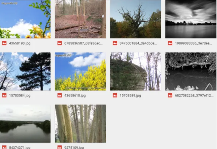
The specific photos which were mislabelled in this way were identified and investigated, and are shown in Figure 3. It can be seen that, while some contain elements such as text or grey-scale colouring which could confuse a scene classifier, others clearly depict natural features such as woodland. On these photo-graphs, the UW approach performed much better, classifying all as natural. A likely explanation is the
Table 7. confusion matrix, precision, recall and f1-score produced on a stratified test set, with number of photographs equal to 25% of all photographs in the paris data set (the remainder were used for training the model) for the Dt approach.
Actual class
Predicted class
Precision Recall F1-score
b bi hf hl n u b 84 0 6 3 0 4 0.79 0.87 0.82 bi 4 10 0 0 0 0 0.71 0.71 0.71 hf 6 0 34 2 1 1 0.57 0.77 0.65 hl 9 0 7 31 0 2 0.86 0.63 0.73 n 0 0 9 0 4 0 0.67 0.31 0.42 u 4 4 4 0 1 12 0.63 0.48 0.55
Table 8. average precision, recall, and f1-score for the Dt approach. Unweighted Weighted precision 0.70 0.73 recall 0.63 0.72 f1-score 0.65 0.72 Downloaded by [79.110.203.215] at 07:30 27 October 2017
which had been labelled ‘useful’, meaning that in total, 427 images were proposed by the model as being use-ful for further interpretation, and only 53 were wrongly rejected.
In this model, we put more weight on ‘useful’ images, thus limiting the number of false negatives, i.e. photo-graphs that were falsely rejected by the algorithm as ‘not useful’. By tuning the weights in the other direction (Table 10), we could reduce the number of images pro-posed by the model for further analysis to 302, but at the cost of rejecting a further 75 photographs which a human had labelled as potentially useful. In this model, the exact location associated to the photograph. We had
similar difficulty in deriving this particular definition of ‘usefulness’ by both classification strategies, since both UW and DT methods are specifically identifying and reporting features which may be at some distance from the photographer.
When trained and cross-validated with a fivefold approach on the London images, the DT approach achieved reasonable results (overall accuracy of 86%) but on the Paris data set it performed badly, with accuracies of 55%. This is unsurprising when we consider that the algorithm was trying to learn and generalize the rules behind several steps of human reasoning, some of them rather subjective. In trying to learn how the experts had classified ‘usefulness’, the DT approach assigned relative weighting to the scene attributes and categories. These generally correspond to highly informative factors in land cover identification: such as ‘plaza’, ‘crosswalk’, ‘sky-scraper’, ‘river’, ‘shopfront’, ‘formal garden’ and ‘field/ wild’ (all of which feature as key deciding factors in the derived classification).
By setting weights on the model, we could manipu-late its sensitivity and specificity, and could control how strict the algorithm should be in rejecting photographs as not useful. In Table 9, we show an example in which we gave ‘useful’ images more weight to limit the incor-rect rejection of pictures. This resulted in the accept-ance for further analysis of 76 pictures which had been considered ‘not useful’ by the human expert, and 351
Figure 3. photographs mislabelled by the Dt method for identifying human impact in a landscape.
Table 9. confusion matrix, and the precision, recall, and f1-score for the “usefulness” prediction with the Dt approach. Actual
Predicted
Precision Recall F1-score
No Yes
no 118 76 0.82 0.87 0.84
Yes 53 351
Table 10. confusion matrix, and the precision, recall, and f1-score for the “usefulness” prediction with the Dt approach by tuning the weights such that we limit the number of false positives (increasing precision at the expense of recall). Actual
Predicted
Precision Recall F1-score
No Yes
no 168 26 0.91 0.68 0.78
Yes 128 276
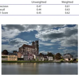
private and transport units’ (class 12), which is hardly surprising given how semantically close they are. Also, higher error rates are present when it comes to misclas-sifying built-up areas as water bodies (class 50). In the majority of cases, this stems from the fact that in many urban photographs whose geolocation indicates a built land cover, a river is the object of interest (Figure 4). This tendency for photographs to include distant objects, which may, in fact, be informative, was the motivation for us to consider classes in the neighbouring vicinity in Goal 4.
Figure 4 was recognized by the DT method as class 50 (Water), though the UA label for the photograph’s location is 12 (Industrial, commercial, public, military, private and transport units). Although the photogra-pher was clearly standing on the bank of the river, the algorithm cannot infer this fact, and makes its classifi-cation based only on information present in the image itself.
3.2.4. Goal 4: identifying UA land cover classes in the surrounding area
One of the potential pitfalls of using labels which are co-located with a given photo is that they will not nec-essarily accurately represent the image’s content. A photo of a forest can be taken from a wetland, which will result in misclassification: the algorithm will, cor-rectly, recognize trees and predict class ‘Forest’ instead of ‘Agricultural areas, semi-natural areas and wetlands’. To address it, we also considered the buffer around the spot from which the picture was shot. If we find that we put more weight on ‘not useful’ images, thus limiting
the number of false positives, i.e. photographs that were incorrectly accepted by the algorithm as ‘useful’.
The UW approach was specifically designed to build in the steps of land cover classification from the original paper and then to derive definitions of ‘usefulness’ from a strict application of the rules in Table 3. This approach performed acceptably on the London images (71.31% accuracy) but did not equal the performance of the DT algorithm. The UW approach performed particularly badly when extended to the Paris data set, with accura-cies of 48% at most. This was little better than random, even when the analysis was reduced to two classes by collapsing the ‘maybe’ photographs into the ‘not useful’ class (Table 11).
3.2.3. Goal 3: identifying land cover as defined by UA
To address this goal, we again looked at scene catego-ries, scene attributes and output of penultimate layer of the neural network. Using the DT approach, we built separate models for level 2 and level 4 UA categories for the Paris region, based on 1880 labelled photographs. In Table 12, we see that the results are quite poor, mostly due to having huge class imbalances and tiny numbers of samples on which to train many of the classes (Tables 5 and 6). Level 2 is better predicted than level 4, largely because of the aggregation of urban classes to higher level masks confusions between the varying mixes of built-up surface. Prediction accuracy of the selected predictors is shown in Table 13, with average precision, recall, and F1-score are presented in Table 14.
In general, the algorithm does a good job at recog-nizing built-up areas (for example, classes 11 to 14 from UA, Table 4) and distinguishing them from other classes. As can be seen from the related confusion matrix (Table 13), most often the algorithm confuses ‘urban fabric’ (class 11) with ‘industrial, commercial, public, military,
Table 11. confusion matrix, precision, recall and f1-score for the “usefulness” prediction with the UW approach.
Actual
Predicted
Precision Recall F1-score
No Yes
no 411 164 0.56 0.53 0.54
Yes 180 206
Table 12. confusion matrix for Ua level 2 and the class prediction based on the scene attributes.
notes: Here, 11 = Urban fabric, 12 = industrial, commercial, public, military, private and transport units, 13 = mine, dump and construction sites, 14 = artifi-cial non-agricultural vegetated areas, 20 = agricultural areas, semi-natural areas and wetlands, 30 = forests, 50 = Water.
Actual class
Predicted class
Precision Recall F1-score
11 12 13 14 20 30 50 11 43 51 0 4 4 1 2 0.54 0.41 0.46 12 27 186 0 8 3 0 4 0.69 0.82 0.75 13 0 2 0 1 0 0 0 0 0 0 14 1 15 0 23 3 2 5 0.53 0.47 0.50 20 4 6 0 5 14 2 4 0.54 0.40 0.46 30 1 2 0 1 0 3 1 0.38 0.38 0.38 50 4 8 0 1 2 0 27 0.63 0.64 0.64
Table 13. prediction accuracy of land cover with the Dt approach on the extraction of Ua classes from photographs, considering level 2 classes (7 classes) and level 4 classes (14 classes). “chance of getting the result at random” is simply the chance of randomly guessing the class, 1/7th and 1/14th respectively.
Predictor Accuracy (%)Level 2 Accuracy (%)Level 4
scene categories 63.19 48.09
scene attributes 62.77 50.43
penultimate layer of the neural
network 64.26 52.13
chance of getting the result at
random 14.29 7.14
shows that they may have different merits and may even complement one other.
When applied to assessing ‘usefulness’, the DT algo-rithm managed to capture essential rules behind the concept of ‘usefulness’ for the training set, but failed to generalize them to an independent set of images from another geographical location. We speculate that the method could still be considered valuable for certain scenarios in which experts classify a relatively small and evenly sampled set and then use it to train a model that is going to be used to filter for ‘usefulness’ a second set from the same area, possibly much larger. However, the rules defining ‘usefulness’ need to take into account the strengths and weaknesses of photographs acquired at ground level: for example, their potential for identify-ing features within a radius, or combinations of land covers which together constitute a specific land use. In addition, there are many cases where an automated algorithm cannot infer anything about the viewpoint of a photographer, while a human observer would be able to extract reasonably accurate information. A valuable cue in identifying these photos is the conflict between existing land cover labels and those assigned by the neu-ral network. Such conflicts can be exploited by preferen-tially presenting these photographs to users for further interpretation.
There are many situations where a photograph can be labelled using an existing land use map, but the accuracy of the photo’s location and the currency of the underly-ing map are in doubt. Ground-acquired photos whose acquisition date is known have a particular potential for identifying recent and dynamic changes which take time to filter into authoritative maps, and which may not be picked up by dynamic crowd sourced resources such as OpenStreetMap. In these cases, both the label assigned by automated overlay with existing maps and the features identified using a neural network could be combined as priors in more sophisticated Bayesian mod-els which identify the key photographs for human inter-pretation, using contextual rules and apparent conflicts. By tuning the DT algorithm, a user can define how strict in rejecting photographs the model should be. This is an important feature, since the risk or cost of false negatives and positives varies between use cases. For example, in a game-oriented photograph-identification application where plentiful pictures are available for a location, it is important to maintain user engagement by presenting them with only the most interesting and rele-vant pictures to interpret. By contrast, in a context where photographs are sparse but each one might contain crit-ical information (for example, on earthquake damage or an invasive species) the cost of wrongly rejecting images as “non-informative” is much higher.
The application of the neural network to identify the land use / land cover classes used in UA on the photo-graphs when only the photograph footprint was con-sidered showed to have accuracies a little higher than the predicted class is among the classes within a buffer,
then we consider it a match. Such approach significantly boosts accuracy, but also adds considerable odds that we will get a correct result purely by chance. However, the results achieved by the DT approach (Table 15) were still significantly above those which could be achieved by chance.
In Table 15, the higher chance of getting the result at random in a larger buffer is due to the larger number of classes that can be present in a given radius. The chance of getting the correct answer at random is calculated using the average number of classes per photo divided by the total number of classes.
3.3. Discussion
In the assessment of human impact, both DT and UW algorithms showed advantages and disadvantages, as they performed differently when applied to photographs from a region other than the one used for training. This
Table 14. average unweighted and weighted average of the precision, recall, and f1-score for the level 2 Ua classes pre-sented in table 11.
Unweighted Weighted
precision 0.47 0.61
recall 0.44 0.63
f1-score 0.45 0.62
Figure 4. the example of urban photographs whose geolocation indicates objects which is not the objects of interest.
Table 15. prediction accuracy of land cover with the Dt ap-proach for levels 2 and 4 of Ua classes within 20, 50, and 100 m buffers defined around the photographs’ locations.
Predictor
UA level 2 UA level 4 20 m 50 m 100 m 20 m 50 m 100 m buffer
(%) buffer (%) buffer (%) buffer (%) buffer (%) buffer (%) scene categories 86.38 91.28 94.04 61.49 68.09 80.00 scene attributes 85.53 90.43 94.04 64.89 70.85 80.43 penultimate layer
of the nn 85.96 90.21 92.98 66.38 73.19 82.13 chance of
get-ting the result at random
25.88 30.69 38.59 16.36 21.62 29.29

![Table 8. average precision, recall, and f1-score for the Dt approach. Unweighted Weighted precision 0.70 0.73 recall 0.63 0.72 f1-score 0.65 0.72 Downloaded by [79.110.203.215] at 07:30 27 October 2017](https://thumb-us.123doks.com/thumbv2/123dok_us/1990338.2795667/12.892.457.802.376.440/average-precision-approach-unweighted-weighted-precision-downloaded-october.webp)