The Predictive Power of Futures Prices and Realized Volatility
Kristian Hoff
Magnus Olsvik
Industrial Economics and Technology Management
Supervisor: Peter Molnar, IØT
Co-supervisor: Ragnar Torvik, ISØ
Department of Industrial Economics and Technology Management Submission date: June 2015
The analysis addresses some of the key questions that arise in forecasting the price of crude oil. Does there exist a methodology which is more accurate than the no-change forecast? Is it possible to extract information from the price of crude oil futures? What other variables may predict future movements in the oil price? Which model provides the greatest directional accuracy?
Assignment given: 12th January 2015 Supervisor: Postdoc Peter Molnar Co-supervisor: Professor Ragnar Torvik
This thesis is written as the conclusion of the Master’s programme in Industrial Economics and Technology Management at the Norwegian University of Science and Technology (NTNU), Trond-heim, during the spring of 2015. We have specialized in Empirical and Quantitative Methods in Finance, writing the thesis within the field of oil price forecasting, due to both personal as well as academic interests.
The analysis is conducted mainly using software such as EViews and Microsoft Excel. The Master’s thesis is written in the form of an article with the purpose of publishing in a scientific journal. We would like to thank our supervisor Postdoc Peter Molnar for providing valuable discussions. Thanks are also directed to co-supervisor Professor Ragnar Torvik who has contributed with useful comments. Responsibility for any errors in this Master’s thesis lies with the authors alone.
Trondheim, June 4th 2015
Denne studien tar for seg predikerbarheten av spotprisen på råolje ved bruk av futurespriser og spot-prisenes realiserte volatilitet. Prognoser basert på dagens spotpris viser seg å være mer nøyaktige på kort sikt enn prognoser basert på futurespriser. Over lengre horisonter er futures-baserte prognoser bedre enn spotpris-prognoser. Både prognoser basert på dagens spotpris og prognoser basert på futurespriser kan forbedres ved å inkludere realisert volatilitet som forklaringsvariabel. Videre kan realisert volatilitet predikere endringer i futurespriser. Samlet viser analysen at realisert volatilitet spiller en viktig rolle ved generering av prognoser for oljepriser.
The Predictive Power of Futures Prices and Realized Volatility
Kristian Hoff
1and Magnus Olsvik
11 Department of Investments, Finance and Economics,
Norwegian University of Science and Technology
E-mail: kristian.hoff@gmail.com, olsvikmagnus@gmail.com
Abstract
This paper studies the predictability of the crude oil spot price using futures prices and realized volatility of spot prices. Over the short-term, the simple no-change forecast works better than forecasts based on futures prices. Across long-term horizons futures-based forecasts perform better than the no-change forecast. Both these types of forecasts, the simple no-change forecast and forecasts based on futures prices, can be improved by incorporating realized volatility as an additional predictor. Moreover, realized volatility can also predict changes in futures prices. Altogether, realized volatility plays an important role in forecasting oil prices.
1
Introduction
Due to the global importance of oil, accurate spot price forecasts are in the interest of numerous agents, not oil-related businesses exclusively. Intuitively, the futures market should provide an idea of the expected future spot price. Market participants commonly assume that futures prices include all available information, thus representing their best available forecast of the spot price. Simple forecasts based on futures prices are often considered satisfactory. The alternative is developing a more advanced prediction model, a relatively time-consuming and resource-intensive exercise, not being guaranteed greater forecast accuracy.
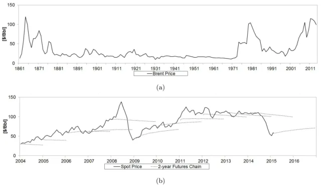
From the early 20th century until the 1970s the price of crude oil was relatively stable. The nature of oil prices shifted in 1973, when volatility increased dramatically. Since then the volatility of crude oil prices has been high. The variability of the Brent spot price is illustrated in Figure 1a, indicating substantial price fluctuations particularly after the establishment of OPEC.
The price of oil is significantly affected by trends in the world economy and geopolitical events. These features renders the oil price inherently unpredictable. Hamilton (2008) describes the price of crude oil in the following manner: “It is sometimes argued that if economists really understand something, they should be able to predict what will happen next. But oil prices are an interesting ex-ample (stock prices are another) of an economic variable which, if we really understand it, we should be completely unable to predict.” The predictive content of futures prices, in terms of predicting unrealized spot prices, is illustrated in Figure 1b. Two-year forward curves are superimposed upon the historical Brent spot price between 2004 and 2015. This figure shows that market expectations rarely are right.
As mentioned, the broad extent of factors impacting the crude oil market increases the efforts of forecasting future prices. Multiplier effects and feedback loops may contribute to further dilute forecasts. All of these uncertainties will affect the estimates differently, depending on the approach undertaken. Several different forecasting methodologies exist, the majority resting on various types of historical time series modelling. These models typically consider price dynamics in the short-run, that is, 1-2 years ahead.
The following explores different models forecasting the price of crude oil, examining the ex-planatory power embedded in prices of futures contracts and in realized volatility. The analysis concentrates on time series modelling, assessing the performance of specific predictors of the Brent spot price. Ultimately, the purpose is determining the forecast model producing the most accurate estimates.
(a)
(b)
Figure 1: (a) Brent price, 1861-2014. (b) Spot price compared to forward curves, 2004-2015.
The analysis addresses some of the key questions that arise in forecasting the price of crude oil. Does there exist a methodology which is more accurate than the no-change forecast? Is it possible to extract information from the price of crude oil futures? What other variables may predict future movements in the oil price? Which model provides the greatest directional accuracy?
This paper makes two main contributions to existing literature. First of all, the analysis extends the study of Alquist and Kilian (2010) by considering a wider range of spreads and relations which may be strong predictors of future spot prices. The study increases the number of contracts by including maturities up to five years. Simultaneously, a larger and more recent data sample spanning from July 1988 to February 2015 is investigated. In accordance with Alquist and Kilian (2010), futures prices are found not to improve no-change forecasts across forecast horizons up to one year. However, for long-term contracts, which were not studied by Alquist and Kilian (2010), the opposite result is attained. Second, the study also considers the forecasting power of realized volatility and finds that it is a useful predictor of oil prices. Realized volatility improves forecasts of not only spot prices, but also returns of futures contracts.
Oil price forecasting is an area of study which has been subject to extensive research over the years. Thus, literature is abundant. The majority of existing literature restricts its scope to
the short-run. Furthermore, most studies perform historical time series analyses applying Vector Autoregression (VAR) methodologies (see e.g. Kilian and Murphy (2012)). Numerous studies make comparisons between historical price evolutions and trends in factors such as economic activity, oil production, oil inventories, and oil reserves (Baumeister et al., 2013; Pagano and Pisani, 2009; French, 2005). Another strand of literature considers long-term dynamics, invoking fundamentals of supply and demand in order to determine the future equilibrium price levels (Arezki et al., 2014; Cooper, 2003; Pindyck, 1999). This approach involves modelling oil prices using the fundamental relationship between price, volume and price elasticity. The relationship between oil reserves, production, and prices is also important in existing research. Since the subsequent analysis particularly focuses on the first of these approaches, the literature under consideration mainly involves short- to mid-term time series analysis, and similar research.
Policy institutions, including several central banks and the International Monetary Fund, com-monly use the price of NYMEX oil futures as a proxy for the market’s expectation of the spot price of crude oil (Baumeister and Kilian, 2012; Svensson, 2005; IMF). For this reason, several authors study whether futures contracts can be considered a good predictor for the spot price. Arezki et al. (2014) finds that futures contracts do not provide much guidance for medium- and long-term prices, since the contracts either do not go out far enough or the markets are not deep enough. About 20 years earlier, Peck (1985) argued that spot and futures prices reflect expectations almost equally. Yet, sev-eral decades before this paper was published, Working (1942) criticized the view that futures prices reflect economists’ expectations while spot prices supposedly do not incorporate all expectations. Hubbard (1986) integrates short-run and long-run approaches to oil price determination, empha-sizing the two-price structure of the world oil market with coexisting short-term spot prices and long-term futures prices. Alquist et al. (2013) compares the futures price forecast to the no-change forecast. This study finds that the no-change forecast of the real price of oil is the predictor with the lowest mean-squared prediction error (MSPE) at horizons longer than one year, while futures prices improve forecasts over shorter horizons. Further, evidence is presented that adjusting the no-change forecast for the real price of oil for expected inflation significantly increases forecast accuracy of the nominal price of oil at horizons of several years. Another paper which investigates the relationship between crude oil futures prices and the no-change forecasts in-depth is Alquist and Kilian (2010). The study suggests that contract prices tend to be less accurate in the MSPE-sense than no-change forecasts. This result is driven by the oil futures spread, that is, the variability of the futures price about the spot price. The spread typically declines as uncertainty about future oil supply shortfalls increases. The following analysis will to a great extent focus on the method introduced by Alquist and Kilian (2010) and extends this analysis to contracts with longer maturities.
Abosedra and Baghestani (2004) studies crude oil futures prices for maturities up to one year. They find that futures prices are unbiased forecasts of the spot at all maturities investigated, and only the 1-month and 12-month contracts outperform the naive (i.e. the no-change) forecast. These findings are opposed by Moosa and Al-Loughani (1994) which claims that futures prices are neither unbiased nor efficient forecasts of spot prices. Further, Gülen (1998) finds the posted spot price to have predictive information only at short horizons, and that futures prices are efficient predictors of the spot price. Extending to futures contracts on other petroleum products (crude oil, heating oil and gasoline), Bopp and Lady (1991) compares forecasts of lagged spot prices and futures prices. Spot prices were found to provide similar forecasting significance as futures prices, but the latter anticipated seasonal patterns more correctly. In order to forecast the future oil price, today’s spot price is concluded to perform equally well as the futures price.
The use of futures prices as a predictor is questioned in Knetsch (2007). Specifically, the assumption of futures prices being an unbiased predictor of oil prices is investigated. The study evaluates forecasts between one and eleven months ahead, and employs forecast accuracy measures such as root-mean-square error (RMSE), mean error and correct direction-of-change prediction. Furthermore, Knetsch (2007) concludes that futures prices should not be used as a direct predictor due to its lack of predictive power. On the other hand, McCallum and Wu (2005) proves that important information is present in futures prices, especially when considering the spread between spot and futures prices. They note, however, the substantial estimation errors produced by both forecasting methods.
Literature on the link between realized volatility and the oil market is scarce. However, this relationship has to a greater extent been studied for the stock market. Ammann et al. (2009) docu-ments a highly significant relation between stock returns and lagged implied volatility. Nevertheless, they find that lagged historical volatility in contrast do not carry the same informational content as implied volatility. Similarly, Bollerslev et al. (2009) provides evidence that stock market returns are predictable by the difference between implied and realized variances, the variance risk premium, with high (low) premia predicting high (low) future returns. Examining the effect of VIX levels on stock market index returns, Banerjee et al. (2007) finds a positive relationship, thus confirming the forecasting power of implied volatility for future returns of stock portfolios. Chevallier and Sévi (2013) builds on the findings of Bollerslev et al. (2009), establishing the predictability of the variance risk premium for crude oil returns. Their results indicate strong explanatory power of this factor on excess returns of oil futures.
The rest of the paper is organized as follows. Section 2 introduces specifications of oil futures contracts and provides a data description. Section 3 evaluates forecasting models for the spot price of
oil. Section 4 considers models using realized volatility to predict changes in futures prices. Section 5 concludes.
2
Data
Futures contracts represent indicators of market expectations for the future spot price of oil. These contracts are financial instruments that lock in a price at a predetermined future date at which to buy or sell a fixed quantity of the commodity. The NYMEX light sweet crude (WTI) contract is the most liquid and largest volume market for crude oil trading (CME Group, 2015-04-13). However, since the Brent oil has increasingly become the benchmark among market actors, and also due to the logistical issues related to Cushing, OH, the delivery hub of WTI, the Brent crude contracts are analyzed in this study.
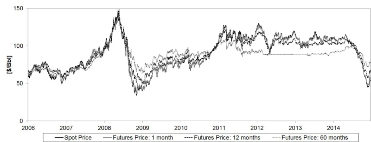
Focus will be on futures traded on the NYMEX (The New York Mercantile Exchange) with monthly price data retrieved from EcoWin. The datasets are constructed from the historical futures chain of each month. Hence, the aggregate of the individual futures chains comprises a time series of monthly futures prices for every contract. The analysis deals with monthly data for oil returns because returns at higher frequencies are too noisy (see e.g. Baumeister and Kilian (2012) or Alquist and Kilian (2010)). The data sample for the first position (the 1-month contract) starts in July 1988 and extends to February 2015 (∼7040 trading days). Contracts of longer maturity are less liquid, with the samples becoming gradually available between July 1988 and March 2006. The contract maturities range up to five years, with maturities exceeding one year becoming available from 2005 onwards. The contract types specifying physical, as opposed to financial, delivery are analyzed here. Trading of the futures contracts ends one business day prior to the termination of the Brent futures contract, that is, two business days before the fifteenth calendar day prior to the first day of the delivery month, as long as the fifteenth calendar day is not a holiday or weekend in London. If the fifteenth calendar day is a holiday or weekend in London, trading shall end three business days prior to the last business day preceding the fifteenth calendar day (CME Group, 2015-03-06). Monthly spot price data are obtained from EcoWin and refer to the price of Brent crude oil available for delivery at Sullom Voe, Scotland. Figure 2 plots the daily prices of crude oil futures contracts for the 1-month, 1-year, and 5-year maturities, along with the spot price starting 24 February 2006. Figure 3 shows daily trading volume of futures contracts with maturities up to three years. Clearly, the markets for contracts of longer maturities are still relatively illiquid. The low trading volume of long-term contracts may imply that forecasts based on longer maturity contracts risk a higher degree of uncertainty.
Figure 2: Historical prices of the Brent spot and Brent futures contracts over the period February 2006 – February 2015.
(a) 1-month futures contract (b) 3-month futures contract (c) 6-month futures contract
(d) 1-year futures contract (e) 2-year futures contract (f) 3-year futures contract
Figure 3: Trading volume of NYMEX crude oil futures contracts for maturities between one month and three years. The 4-year and 5-year contracts are exempt due to few data points. Note the different scales on axes.
This paper utilizes the realized volatility of Brent prices. Daily spot price returns of the preced-ing month provide spot-based estimates of realized volatility. Likewise, realized volatility of futures is constructed from the daily returns of the respective contract over the preceding month. The estimator of realized volatility at timetis defined as in equation (i).
RVt = n
X
i=1
r2i, (i)
whereri are daily returns and nis the number of trading days of the preceding month. Thus, the
sum of ex-ante daily squared returns provides the estimates for realized volatility of spot prices and eight different futures contracts.
3
Spot Price Forecasting
This section examines different methods of forecasting the spot price of crude oil. First, the predictive power of futures prices is investigated. Next, the analysis considers an expansion of the models to include realized volatility as an explanatory variable.
3.1
Predictive Power of Futures Prices
The futures price of oil is often considered a proxy for the expected price of oil in the future. Some also believe futures contracts are better predictors than econometric forecasts, especially contracts that are actively traded. The notion that the futures price might be the optimal forecast for the spot price is a by-product of the financial market efficiency hypothesis: the requirement that the average forecasting error is zero is consistent with both efficiency in financial markets and the unbiasedness property of the forecast (Pagano and Pisani, 2009).
A price forecasting model is presented where eighteen unique relations explaining the future spot price of crude oil are tested using an OLS regression model. The performance of each model is tested by calculating prediction accuracy measures used in literature, such as root-mean-square error (Knetsch, 2007; Inoue and Kilian, 2006) and bias (Alquist and Kilian, 2010). Comparisons of the relations to the no-change model are based on the DM-test of Diebold and Mariano (2002), providing statistical significance levels for the error estimation. The sign test given by the success ratio indicates the directional accuracy of the forecasts.
Alquist and Kilian (2010) compares the no-change forecast for the 1-month, 6-month, 9-month and 12-month forecasting horizon with forecasts based on futures prices. They conclude that the no-change forecast outperforms the rest. This section builds upon Alquist and Kilian (2010), extending
the analysis by three new models, (7)-(9), given in the equation set below. In addition, the models are extended to include contracts of longer maturities and a larger sample size. The added contracts include maturities of two, three, four and five years, while the data samples are extended until February 2015.
Let Et[St+h|t] represent the expected future spot price h periods ahead. Thus, Sˆt+h|t is the
estimated future spot price at datet+h, conditional on information available at timet. Denote by Ft(h)the current timetnominal price of futures contracts that mature inhmonths, whileStdenotes
the current spot price of oil. The maturities, h, range from one month to five years. In line with Alquist and Kilian (2010), the equation set includes the following forecasting models:
ˆ St+h|t = St, h = 1,3,6,12,24,36,48,60 (1) ˆ St+h|t = F (h) t , h = 1,3,6,12,24,36,48,60 (2) ˆ St+h|t = St(1 + ˆα + ˆβ ln(F (h) t /St)), h = 1,3,6,12,24,36,48,60 (3) ˆ St+h|t = St(1 + ˆβ ln(F (h) t /St)), h = 1,3,6,12,24,36,48,60 (4) ˆ St+h|t = St(1 + ˆα+ln(F (h) t /St)), h = 1,3,6,12,24,36,48,60 (5) ˆ St+h|t = St(1 +ln(F (h) t /St)), h = 1,3,6,12,24,36,48,60 (6)
In addition, the following extension is made:
ˆ St+h|t = ˆα + ˆβ F (h) t + ˆγ St, h = 1,3,6,12,24,36,48,60 (7) ˆ St+h|t = ˆα + ˆβ ln(F (h) t /St), h = 1,3,6,12,24,36,48,60 (8) 8
ˆ
St+h|t = ˆα + ˆγ St, h = 1,3,6,12,24,36,48,60 (9)
The first model considered is the no-change forecast, equation (1). The analysis also examines models based on the price of oil futures, first by testing the futures price as a direct predictor of the spot price, see (2). Next, equations (3)-(6) represent a more relaxed set of models. Similarly, equations (7) and (8) state that the future spot price is represented by the sum of a constant,αˆ, and a slope term multiplied by the explanatory variable. Finally, equation (9) serves as a relaxed version of the no-change model.
Table 1 presents in-sample coefficient estimates from the regression model, covering the whole sample. The most liquid contracts, that is, the 1-month, 3-month and the 6-month contracts, are presented in this table. Apparently, not every coefficient is statistically significant, still, these estimates are good compared to alternative models tested. Particularly equations (7)-(9) generate significant results, indicating that these are reliable models. The regression results are adjusted by the Newey-West procedure for autocorrelation and heteroskedasticity (Newey and West, 1986). The Akaike Information Criterion (AIC) is also reported in Table 1. Given a set of candidate models for the data, the preferred model is the one with the minimum AIC value (Alexander, 2009).
For the purpose of comparing forecasts, the root-mean-square errors (RMSE) are calculated for all eight contracts. The simple no-change forecast is specified as a benchmark model. The RMSE of a prediction is given by the square root of the mean of the squared deviations (Knetsch, 2007), as presented in equation (ii). The bias is another error measure which is defined as the average amount by which the true value,St+h, exceeds the prediction, see equation (iii). All p-values refer to pairwise
DM-tests where the null hypothesis is a zero difference in forecasting errors between the no-change benchmark and the forecast. The DM-test indicates whether the difference in errors is significantly different from zero. The success ratio is defined as the fraction of forecasts that correctly predict the sign of change in the price of crude oil. Hence, the success ratio gives an indication of the directional accuracy of the predictions.
RM SE = v u u t n P t=1 ( ˆSt+h|t− St+h)2 n (ii) Bias = n P t=1 (St+h− Sˆt+h|t) n (iii)
T able 1: In-sample co efficien t estimates for the 1-mon th, 3-mon th and 6-mon th con tracts. The AIC is pro vided for eac h maturit y . *, ** denote statistical signific ance at resp ectiv ely the 5% and 1% lev els. h = 1 h = 3 h = 6 ˆ S t + h | t α β γ AIC α β γ AIC α β γ AIC (1) S t (2) F ( h ) t (3) S t(1+ ˆ α + ˆ β ln( F ( h ) t / S t)) 0.00 -0.50 6.13 -0.01 -0.74 7.48 -0.01 0.26 8.30 (4) S t(1+ ˆ β ln( F ( h ) t / S t)) -0.49 6.13 -0 .72 7.48 0.30 8.30 (5) S t(1+ ˆ α +ln( F ( h ) t / S t)) 0.00 6.21 -0.01 7.63 -0.01 8.31 (6) S t(1+ln( F ( h ) t / S t)) (7) ˆ α + ˆ β F ( h ) t + ˆ γ S t 0.79* -0.56 1.54* 6.13 2.63* -0.78 1.73* 7.46 5.23* 0.23 0.69 8.26 (8) ˆ α + ˆ β ln( F ( h ) t / S t) 46.36** -105.70 9.98 46.52** 12.02 9.99 48.24** 28.25 10.00 (9) ˆ α + ˆ γ S t 0.65* 0.99** 6.1 3 2.51* 0.96** 7.49 5.28* 0.91** 8.25 10
Panel A of Table 2 presents the RMSE for the relations described above. Generally, the differ-ences in RMSE appear relatively small for all equations. The no-change forecast performs best in the short-run, while forecasts based on futures (or a combination of the no-change and futures) are better for longer horizons. Including maturities exceeding 12-months reveals that the no-change fore-cast is outperformed by futures models over longer forefore-cast horizons. Most of these results are also statistically significant. Partially different from the findings of Alquist and Kilian (2010), the results suggest that the no-change forecasts over the 1-month and 3-month horizons generate lower RMSE than forecasts using futures contracts as input. For longer forecasting horizons futures contracts, or models combining futures contracts and the no-change forecast, emerge as better predictors of the future spot price of crude oil. Nevertheless, in accordance with Alquist and Kilian (2010), the RMSE measure indicates that none of the models provide better forecasts than the simple no-change model for horizons up to three months. At horizons ranging from 12 to 36 months, the predictive power of futures models is better than the no-change model, with equation (7) generating the smallest errors. Equation (8) produces the smallest RMSE for the 4-year contract, while relation (7) again is the most accurate forecast for the 5-year maturity. Regarding horizons exceeding one year, models applying futures prices as input are significantly better compared with the no-change forecast. Note that as maturities increase, the liquidity of contracts generally decrease. Overall, less restrictive models (e.g. comparing equation (7) with equation (2)) produce better forecasts.
The bias estimates are displayed in panel A of Table 3. The overweight of positive values suggests that the realized spot price is higher than the forecasted spot price in the majority of cases. This is analogous to Alquist and Kilian (2010) which presents small negative bias results solely for the 1-month contract, all others being positive with absolute values similar to those presented here. The futures model given by equation (5) is the best predictor of future spot prices for forecasting across horizons of 1-month, 3-months, 1-year, 2-years, and 3-years, according to the bias estimates. The bias implies that the most accurate forecast with regards to the 6-month maturity is provided by relation (3). Over the 4-year and 5-year horizon the bias is minimized by applying equation (7). Hence, regarding the bias measure of forecasting errors, it can be concluded that the simple no-change forecast underperforms relative to models incorporating both the no-change and futures forecasts. Alquist and Kilian (2010) finds that the no-change model generates the smallest bias across the 6-month and 12-month horizons, while for the 1-month and 3-month contracts they reach the same conclusion as above.
The success ratio measures the directional accuracy of forecasts. It represents an indicator of the extent to which the forecasting models are able to predict the direction of change, taking a value between zero and one. Panel A of Table 4 presents the success ratio for the different models and
maturities. The greatest performance in terms of directional accuracy is provided by the futures forecast (2) and the relationship given by equation (6), for all horizons except the 5-year maturity. Concerning the 5-year contract, equation (8) provides the best prediction of the direction of future price changes. The differences among models are somewhat greater relative to Alquist and Kilian (2010), but the absolute values for corresponding models and horizons are consistent with the findings of Table 2.
Models combining the futures and no-change forecasts demonstrate the best performance as predictors of future spot prices. These results represent both similarities and differences relative to previous research. Alquist and Kilian (2010) finds that the no-change forecast tends to be the most accurate forecasting method. Other studies have found futures-based forecasts to provide better forecasts at horizons of 3-, 6- and 12-months (Chernenko et al., 2004). Nevertheless, more consistent with the findings presented here, McCallum and Wu (2005) finds that spread regressions, i.e. models incorporating both the futures and the no-change forecast, have lower MSPE than the simple no-change forecast at short horizons.
The no-change forecast tends to be relatively accurate for horizons up to twelve months. This is consistent with existing literature and the view among agents in the oil market. As stated in the introduction, Hamilton (2008) suggests that oil prices are completely unpredictable. Although presenting different results, the no-change model being favoured by Alquist and Kilian (2010), Cher-nenko et al. (2004) favouring the futures model, and the spread regression being favoured by Mc-Callum and Wu (2005), these studies do not contradict each other nor the findings above. The divergence in forecast accuracy can mainly be explained by differences in the sample period. The estimates presented in this section are based on a larger sample size compared to the mentioned studies. Oil price predictability is also affected by a range of factors and the tie to the spot price of oil is, to put it mildly, complicated (Zagaglia, 2010). Thus, the connection between the oil price and macroeconomic determinants is important to bear in mind.
Although futures prices bring a lot to the table, the value of the futures price as a predictor of the expected future spot price may be disputed. As suggested by the historical futures chains superimposed upon the historical spot prices in Figure 1b, futures prices are highly questionable as a direct predictor of future crude oil spot prices. One might argue that the simple no-change forecast in several cases provides a satisfactory forecast of the expected spot prices compared to more complicated models. Nonetheless, spreads combining the futures and no-change forecasts emerge from this analysis as strong predictors of the future spot price.
Various explanatory variables for the price of crude oil have been considered in this study, some by inspiration from existing literature while others are proposed by authors. In addition to
T able 2: RMSE of sp o t price forecasts for differen t equations and maturities. Significan t imp ro v emen t from the no-c hange (1) is giv en b y asterisks, while daggers ( † ) indicate significan t impro v emen t for the pairwise test of (10 )-(18) to w ards the mo dels (1)-(9). */ † , **/ †† denote statistical significance at resp ectiv ely the 5% and 1% lev els. RMSE P anel A h = 1 h = 3 h = 6 h = 12 h = 24 h = 36 h = 48 h = 60 (1) St 5.08 10.10 15.11 20.18 30. 04 29.98 27.96 28.46 (2) F ( h ) t 5.28 10.80 15.34 19.02** 25.39** 24.87** 22.75** 25.19** (3) St (1+ ˆ α + ˆβln( F ( h ) t / St )) 5.23 10.74 15.91 20.22 15.30** 15.87** 18.86** 22.85 (4) St (1+ ˆβln( F ( h ) t / St )) 5.14 10.42 15.33 19.06** 15.82** 17.50** 17.44** 26.11 (5) St (1+ ˆ α +ln( F ( h ) t / St )) 5.39 11.12 15.97 19.57** 18.08** 17.17** 19.57** 22.21** (6) St (1+ln( F ( h ) t / St )) 5.28 1 0.78 15. 35 19.10** 25.66** 25.44** 23.55** 25.81** (7) ˆ α + ˆβ F ( h ) t + ˆ γ St 5.26 10.23 14.71 17.93** 15.31** 15.15** 11.55** 10.06** (8) ˆ α + ˆβln( F ( h ) t / St ) 17.15 16.08 16.31 18.7 7 15.86** 16.28** 11.37** 10.55** (9) ˆ α + ˆ γ St 5.25 10.34 15.12 18.62* 16.37** 16.63** 11.44** 10.83** P anel B h = 1 h = 3 h = 6 h = 12 h = 24 h = 36 h = 48 h = 60 (10) St + ˆδR Vt 5.14 10.34 15.86 20.92 23. 59 24.82 23.11 22.81* † (11) F ( h ) t + ˆδR Vt 5.35 11.08 16.14 19.75 18.36** 17.31** 18.68** 21.33* (12) St (1+ ˆ α + ˆβln( F ( h ) t / St ))+ ˆδR Vt 5.32 10.88 16.56 19.43 †† 14.04** †† 16.26** 19.70** 23.33 (13) St (1+ ˆβln( F ( h ) t / St ))+ ˆδR Vt 5.19 10.78 16.04 20.17 16.58** 16.85** † 18.29** 22.00* † (14) St (1+ ˆ α +ln( F ( h ) t / St ))+ ˆδR Vt 5.42 10.96 16.77 19.79 18.66** 18.58** 20.41* 22.70 (15) St (1+ln( F ( h ) t / St ))+ ˆδR Vt 5.35 11.06 16.16 19.84 18.71** 17.95** 19.35** 21.62* (16) ˆ α + ˆβF ( h ) t + ˆ γ St + ˆδR Vt 5.06 9.04 †† 11.02** †† 15.10** †† 10.09** †† 11.99** †† 9.14** †† 7.51** †† (17) ˆ α + ˆβln( F ( h ) t / St )+ ˆδR Vt 15.60 †† 15.33 †† 15.21 †† 16.45** †† 10.32** †† 10.01** †† 9.00** †† 8.43** †† (18) ˆ α + ˆ γ St + ˆδR Vt 5.04 8.64** †† 10.87** †† 14.97** †† 10.62** †† 11.24** †† 8.56** †† 9.47** †
T able 3: Bias of sp ot price forecasts for differen t equations and maturities. Bias P anel A h = 1 h = 3 h = 6 h = 12 h = 24 h = 36 h = 48 h = 60 (1) S t 0.13 0.37 1.08 3.48 7.80 11.52 14. 37 14.37 (2) F ( h ) t 0.04 0.30 1.21 4.14 7.16 10.24 10. 89 11.53 (3) S t(1+ ˆ α + ˆ β ln( F ( h ) t / S t)) -0.1 7 -0.56 0.18 2.12 5.77 1.28 -3.60 -7.00 (4) S t(1+ ˆ β ln( F ( h ) t / S t)) -0.05 0.50 1.61 4.78 6.64 6.52 4.21 8.68 (5) S t(1+ ˆ α +ln( F ( h ) t / S t)) -0.02 -0.03 0.26 0.66 3 .81 -0.28 -2.68 -5.88 (6) S t(1+ln( F ( h ) t / S t)) 0.05 0.34 1.29 4.39 7.62 10. 78 11.45 12.11 (7) ˆ α + ˆ β F ( h ) t + ˆ γ S t 0.16 0.25 1.33 3.58 6.62 6.06 0.19 -2. 10 (8) ˆ α + ˆ β ln( F ( h ) t / S t) 7. 94 6.44 6.24 8.47 7.11 6.87 0.97 -3.03 (9) ˆ α + ˆ γ S t 0.24 0.70 2.29 4.97 6.89 5.67 -0.80 -2.85 P anel B h = 1 h = 3 h = 6 h = 12 h = 24 h = 36 h = 48 h = 60 (10) S t+ ˆ δ R V t 0.24 0.58 1.15 1.77 4.29 4.01 1.50 -1.81 (11) F ( h ) t + ˆ δ R V t 0.30 0.74 1.37 2.00 4.66 3.31 -1.11 -4.47 (12) S t(1+ ˆ α + ˆ β ln( F ( h ) t / S t))+ ˆ δ R V t -0.38 -0.80 -2.83 1.07 5.35 0.72 -2.85 -5.99 (13) S t(1+ ˆ β ln( F ( h ) t / S t))+ ˆ δ R V t 0.01 -0.10 1.66 3.40 6.60 4.45 -1. 44 -4.31 (14) S t(1+ ˆ α +ln( F ( h ) t / S t))+ ˆ δ R V t -0.39 -1.20 -3.19 -0.24 3.55 -1.46 -2.54 -5.21 (15) S t(1+ln( F ( h ) t / S t))+ ˆ δ R V t 0.30 0.74 1.38 2.05 4.93 3.67 -0.77 -4.05 (16) ˆ α + ˆ β F ( h ) t + ˆ γ S t+ ˆ δ R V t 0.22 0.17 0.04 1.05 2.63 3.46 -0.39 -1.88 (17) ˆ α + ˆ β ln( F ( h ) t / S t)+ ˆ δ R V t 7.13 6.41 5.23 5.81 2.32 2.07 -0.74 -3.00 (18) ˆ α + ˆ γ S t+ ˆ δ R V t 0.25 0.06 -0.46 2.66 3.82 2.46 -2. 78 -3.00 14
T able 4: Success ratio of sp ot price forecasts for differen t equations and maturities . V alues represen t the fraction of forecasts that correctly pr e dict the direction of price changes. Success Ratio P anel A h = 1 h = 3 h = 6 h = 12 h = 24 h = 36 h = 48 h = 60 (1) St n.a. n.a. n. a. n.a. n.a. n. a. n.a. n.a. (2) F ( h ) t 0.53 0.50 0.56 0.58 0.62 0.50 0.39 0.23 (3) St (1+ ˆ α + ˆβln( F ( h ) t / St )) 0.04 0.08 0.09 0.21 0.29 0.29 0.50 0.5 0 (4) St (1+ ˆβln( F ( h ) t / St )) 0.03 0.08 0.03 0.21 0.31 0.25 0.05 0.10 (5) St (1+ ˆ α +ln( F ( h ) t / St )) 0.05 0.10 0.12 0.19 0.09 0.16 0. 33 0.45 (6) St (1+ln( F ( h ) t / St )) 0.53 0.50 0.56 0.58 0.62 0.50 0.39 0.23 (7) ˆ α + ˆβF ( h ) t + ˆ γ St 0.07 0.15 0.16 0.31 0.27 0.29 0.19 0.55 (8) ˆ α + ˆβln( F ( h ) t / St ) 0 .40 0.31 0.21 0.26 0.29 0. 24 0.19 0.60 (9) ˆ α + ˆ γ St 0.06 0.13 0.18 0.22 0.27 0.18 0.21 0.57 P anel B h = 1 h = 3 h = 6 h = 12 h = 24 h = 36 h = 48 h = 60 (10) St + ˆδR Vt 0.02 0.04 0.06 0.03 0.02 0.04 0.17 0.29 (11) F ( h ) t + ˆδR Vt 0.06 0.13 0.13 0.16 0.16 0.15 0.10 0.40 (12) St (1+ ˆ α + ˆβln( F ( h ) t / St ))+ ˆδR Vt 0.06 0.12 0.17 0.22 0.27 0.31 0.33 0.45 (13) St (1+ ˆβln( F ( h ) t / St ))+ ˆδR Vt 0.03 0.09 0.09 0.18 0.31 0.29 0.29 0.36 (14) St (1+ ˆ α +ln( F ( h ) t / St ))+ ˆδR Vt 0.08 0.14 0.16 0.14 0.09 0.18 0.24 0.40 (15) St (1+ln( F ( h ) t / St ))+ ˆδR Vt 0.46 0.48 0.53 0.68 0.89 0.82 0.83 0.83 (16) ˆ α + ˆβF ( h ) t + ˆ γ St + ˆδR Vt 0.09 0.18 0.18 0.26 0.33 0.42 0.52 0.64 (17) ˆ α + ˆβln( F ( h ) t / St )+ ˆδR Vt 0.40 0.30 0.22 0.22 0.33 0.31 0.60 0.69 (18) ˆ α + ˆ γ St + ˆδR Vt 0.10 0.19 0.17 0.19 0.31 0.31 0.55 0.69
considering spot and futures prices at different lags, the predictive features of U.S. oil inventories (French, 2005), implied volatility of Brent futures options, skewness of Brent spot prices (analogous to the electricity analysis of Haugom and Ullrich (2012)), and realized volatility of Brent spot prices have become subject to study. Realized volatility of the oil futures market is for example used to predict future volatility in Martens and Zein (2004). Due to more significant results, realized volatility is chosen as the variable in focus for the continuing analysis.
3.2
Predictive Power of Realized Volatility
Several of the models studied in section 3.1 indicate strong explanatory power, yielding low forecast errors and good directional accuracy. The following section expands the analysis conducted above by including the historical realized volatility of crude oil spot prices. The following nine equations are studied, all of which incorporate realized volatility as an explanatory variable:
ˆ St+h|t = St + ˆδ RVt, h = 1,3,6,12,24,36,48,60 (10) ˆ St+h|t = F (h) t + ˆδ RVt, h = 1,3,6,12,24,36,48,60 (11) ˆ St+h|t = St(1 + ˆα + ˆβ ln(F (h) t /St)) + ˆδ RVt, h = 1,3,6,12,24,36,48,60 (12) ˆ St+h|t = St(1 + ˆβ ln(F (h) t /St)) + ˆδ RVt, h = 1,3,6,12,24,36,48,60 (13) ˆ St+h|t = St(1 + ˆα+ln(F (h) t /St)) + ˆδ RVt, h = 1,3,6,12,24,36,48,60 (14) ˆ St+h|t = St(1 +ln(F (h) t /St)) + ˆδ RVt, h = 1,3,6,12,24,36,48,60 (15) ˆ St+h|t = ˆα + ˆβ F (h) t + ˆγ St+ ˆδ RVt, h = 1,3,6,12,24,36,48,60 (16) 16
ˆ St+h|t = ˆα + ˆβ ln(F (h) t /St) + ˆδ RVt, h = 1,3,6,12,24,36,48,60 (17) ˆ St+h|t = ˆα + ˆγ St+ ˆδ RVt, h = 1,3,6,12,24,36,48,60 (18)
The equations given above, (10)-(18), are identical to equations (1)-(9) presented in section 3.1, only differing in that an extra term is added; the realized volatility of the Brent spot price. The explanatory features of realized volatility are investigated in order to determine whether this factor can enhance forecasting models.
As mentioned in section 3.1, other variables are also included in the forecasting models, such as inventories, by inspiration from Pagano and Pisani (2009) which uses utilized capacity in U.S. manufacturing as an explanatory variable and Chevallier (2013) which considers inventories as a predictor of futures returns. However, inventories do not improve the results. The explanatory power of implied volatility of Brent options futures has been tested in the models, examining the CBOE Crude Oil Volatility Index (OVX) ETF, but the results favour the use of realized volatility. Another benefit from using realized volatility as opposed to implied volatility is that this does not restrict the data sample size, as OVX index data is only available from 2007. Adding the skewness of spot prices to the models have also been tested by means of improving forecasts. Still, the value of skewness as a predictor for future spot prices has proved insignificant. For the sake of brevity, these results are not reported in this paper.
In-sample estimates for the 1-month, 3-month and 6-month contracts over the entire sample are presented in Table 5. As mentioned, the termˆδRVt is added to the equations given in section 3.1.
Similar to Table 1, the estimates suggest that not all coefficients are statistically significant. Among the models yielding significant coefficients are equation (16), (17) and (18), that is, the most flexible models. The AIC is also provided in Table 5, where the criterion suggests that the best model fit is obtained from relation (16) and (18) for the most liquid contracts.
Table 2 illustrates the results from adjusting the models in section 3.1. The RMSE for relations (10)-(18) are shown in panel B of Table 2. A dagger (†) indicates significant improvement in RMSE by including historical realized volatility in the relations describing future spot prices. Thus, daggers specify that adding realized volatility as an explanatory variable reduces forecast errors. Considering horizons beyond six months, forecasts are improved by adding realized volatility to the majority of models, with a notable number of error reductions being significant. Examining equations (7)-(9) reveal that adding historical realized volatility to these models unambiguously improve the forecasts
able 5: In-sample co efficie n t estimates for the 1-m o n th, 3-mon th and 6-mon th con tracts. The AIC is pro vided for eac h maturit y . ** den o te statistical significance at resp ectiv ely the 5 % and 1% lev els. h = 1 h = 3 h = 6 ˆ S t + h | t α β γ δ AIC α β γ δ AIC α β γ δ AIC (10) S t + ˆ δ R V t -2.85 6.13 -6.33 7.50 -7.53 8.29 (11) F ( h ) t + ˆ δ R V t -4.13 6.21 -8.63 7.63 -7.58 8.31 (12) S t (1+ ˆ α + ˆ β ln( F ( h ) t / S t ))+ ˆ δ R V t 0.00 -0.47 -1.89 6.13 -0.01 -0.73 -1.24 7.49 -0.01 0.27 -4.10 8.30 (13) S t (1+ ˆ β ln( F ( h ) t / S t ))+ ˆ δ R V t -0.46 -2.31 6.13 -0.70 -5.15 7.48 0.29 -7.27 8.30 (14) S t (1+ ˆ α +ln( F ( h ) t / S t ))+ ˆ δ R V t 0.00 -5.66 6.21 0.00 -9. 52 7.63 0.00 -7.23 8.32 (15) S t (1+ln( F ( h ) t / S t ))+ ˆ δ R V t -4.01 6.21 -8.03 7.62 -6.65 8.31 (16) ˆ α + ˆ β F ( h ) t + ˆ γ S t + ˆ δ R V t 3.11** -0.40 1.38* -21.41** 6.10 8.48** -0.51 1.45* -54.94* 7.40 16.85* 0.50 0.40 -109.51 8.14 (17) ˆ α + ˆ β ln( F ( h ) t / S t )+ ˆ δ R V t 64.48** -55.64 -189.53** 9.92 65.72** 38.01 -199.01** 9.92 69.19** 39.8 6 -215.38** 9.92 (18) ˆ α + ˆ γ S t + ˆ δ R V t 3.19** 0.98** -22.95** 6.10 9.12* 0.94** -61.67 7.41 16.35 0.89** -103.95 8.15 18
for all horizons. Equation (18) provides the lowest error for horizons up to one year. Across the two year and five year horizon, equation (16) generates the lowest errors. Finally, model (17) is favored over long-term horizons of three and four years.
As illustrated by Table 2, models incorporating realized volatility typically perform better. Similar to the findings of section 3.1, models combining futures and no-change forecasts over a given horizon generate the smallest errors. Generally, the simple no-change model is outperformed by these more advanced models. The less restrictive models given by (16)-(18) provide better forecasts than most of the remaining models.
Bias estimates are presented in panel B of Table 3, suggesting that the prediction is higher than the realized spot price for the overweight of models at horizons of four and five years. For maturities over the short- and medium-term the realized spot price is on average higher than the estimated forecast. Comparing the bias estimates to the RMSE, similar conclusions can be drawn; models combining no-change and futures forecasts generally perform better. Nevertheless, the simple no-change forecast is actually preferred across the 5-year horizon. In accordance with the discussion above, realized volatility in most cases contributes to the models by reducing the absolute bias. This implies that the forecasted estimates of models applying information from realized volatility are closer to the realized price compared to models not utilizing this information. The bias estimates do not point out a single best model among equations (10)-(18), as the model generating the minimum bias varies over different horizons. However, equation (16) performs relatively well across all horizons. Indeed, Table 2 confirms significant reductions in RMSE by this model.
Significantly reduced error terms, attained through utilizing the explanatory power of realized volatility, should have an equivalent impact on the success ratio. Panel B of Table 4 indicates mixed results regarding improvements in directional accuracy, relative to the findings presented in panel A. Actually, incorporating realized volatility reduces the success ratio for some models, adopting a 1-month perspective. The same applies to the simple futures model (11) at all maturities except the 5-year horizon. Realized volatility enhances success ratios when forecasting over the medium- and long-term, relative to equivalent models in panel A of Table 4. Considering horizons of one year and above, the model specified by equation (15) stands out by providing superior directional accuracy at more than 80%. The extended futures model (11) provides a higher degree of accuracy in predicting the direction of future price changes, compared to the extended no-change model (10), across the short- to medium-term. In general, all models display improving success ratios as maturities increase. To summarize, there is reason to conclude that predictive information is present in the historical realized volatility of Brent spot prices. To the authors’ best knowledge, this finding on the predictive power of realized volatility is unique and complements existing literature. A direct comparison
between the models in existing research and corresponding models incorporating realized volatility suggests that this extension leads to improved forecasts of the crude oil spot price.
4
Realized Volatility as a Predictor of Futures Returns
Oil futures contracts are typically financial contracts, therefore, this section follows the standard finance literature and turns away from price forecasting and focus instead on predicting the relative movements of futures prices. That is, the analysis considers returns by holding futures contracts of various maturities. Realized volatility is also used by Martens and Zein (2004), although to predict future volatility. Further, Chevallier (2013) uses returns of futures contracts as the dependent variable, this being analyzed with U.S. oil stocks as one of the explanatory variables.
The left hand side of the equations modelled is now the futures return in the next time step,
ˆ
rF(h) t+h|t
, rather than the future spot price as in the previous section. The return variable is calculated as the log-difference between the monthly prices. In an efficient market the futures price should be unpredictable, as opposed to the somewhat predictable spot price, illustrated by the results in section 3. The spot price is likely to be less efficient as transaction costs reduce arbitrage opportunities in the physical market. The futures market is expected to be more efficient since these contracts are both financially and physically settled. Speculation and financial trading may help stabilize futures prices and contribute to an efficient market. Another view is that speculation by financial investors drives futures prices more than spot prices, the latter being more driven by fundamentals, although Singleton (2013) finds that financial activities through holding futures contracts tend to move the spot price away from fundamental values. The consecutive analysis will explore if this intuition is valid.
Forecasting accuracy will be assessed using the RMSE-measure applied in section 3. Significance levels still refer to the pairwise DM-test, providing an indication whether the error improvements are significantly different from zero. The null hypothesis states that the difference in forecasting errors between the zero-return benchmark, (19), and the estimated forecast is zero.
Denote byrˆF(h) t+h|t
the estimated return at timetby holding a futures contract with delivery inh months. RVt,spotdenotes the realized volatility of the Brent spot price, whileRV
(h)
t,f uturesdenotes the
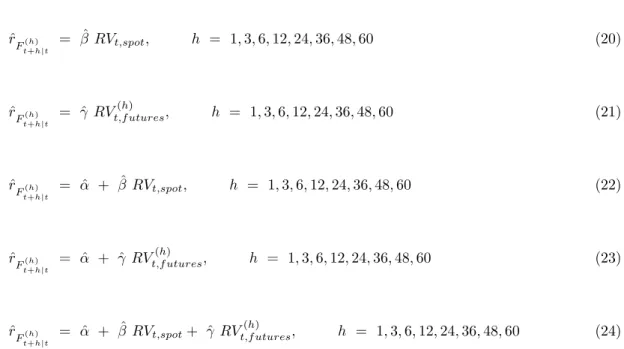
realized volatility of the respective futures contract price. The equation set includes the following forecasting models: ˆ rF(h) t+h|t = 0, h = 1,3,6,12,24,36,48,60 (19) 20
ˆ rF(h) t+h|t = ˆβ RVt,spot, h = 1,3,6,12,24,36,48,60 (20) ˆ rF(h) t+h|t = ˆγ RVt,f utures(h) , h = 1,3,6,12,24,36,48,60 (21) ˆ rF(h) t+h|t = ˆα + ˆβ RVt,spot, h = 1,3,6,12,24,36,48,60 (22) ˆ rF(h) t+h|t = ˆα + ˆγ RVt,f utures(h) , h = 1,3,6,12,24,36,48,60 (23) ˆ rF(h) t+h|t = ˆα + ˆβ RVt,spot+ ˆγ RV (h) t,f utures, h = 1,3,6,12,24,36,48,60 (24)
The first model studied is the zero-return benchmark. Further, the analysis considers two relatively rigid models, equations (20) and (21), stating that historical realized volatility directly predicts contract returns, scaled by a slope term. Equations (22) and (23) represent a more relaxed set of models. Equation (24) is a multivariate model, applying the realized volatility of both spot and futures prices as regressors. This is not expected to be a better performing model, the purpose rather being to determine which factor (realized volatility based on spot prices or based on futures prices) is the most relevant. Hence, the models under assessment are, in addition to the zero-return benchmark, five unique relations applying realized volatility as a predictor of futures returns.
Table 6 shows in-sample estimates, spanning the entire sample size, for the return models applying realized volatility. The least liquid contracts, i.e. the 4-year and 5-year contracts, are omitted in this table. These estimates reveal that, the more relaxed models, (22)-(24), in general perform well across all horizons. Particularly, models (22) and (24) demonstrate the most significant in-sample estimates. The Newey-West procedure for autocorrelation and heteroskedasticity is used to adjust significance levels. In-sample parameters suggest that, in terms of regression significance, models (23) and (22) are favoured for horizons up to and above six months, respectively. The minimum AIC indicates the preferred model, suggesting that model (23) is preferred over horizons shorter than one year. Across horizons of one year and longer the AIC signals that equation (22) outperforms the rest. The estimated slope parameters are negative, implying that higher realized volatility leads to lower returns.
6: In-sample co efficien t estimates for con tract maturities up to 36 mon ths. The AIC is pro vided for eac h maturit y . *, ** statistical significance at resp ectiv e ly the 5% and 1% lev els. h = 1 h = 3 h = 6 F ( h ) t + h | t α β γ AIC α β γ AIC α β γ AIC 0 ˆ β R V t,spot -0.0563 -1.8001 -0.0483 -1.9778 -0.0494 -2. 1502 ˆ γ R V ( h ) t,f utur es -0.0729 -1.8022 -0.0772 -1.9811 -0.0846 -2.1543 ˆ α + ˆ β R V t,spot 0.0486** -0.4653* -1 .8417 0.0452* -0.4283* -2.0213 0.0410* -0.3925 -2.1925 ˆ α + ˆ γ R V ( h ) t,f utur es 0.0509** -0.5127* -1. 8534 0.0480** -0.5296* -2.0390 0.0392* -0.4696 -2. 2053 ˆ α + ˆ β R V t,spot + ˆ γ R V ( h ) t,f utur es 0.0503** 0.0520 -0.5602 -1.8472 0.0475** 0.0247 -0.5527 -2.0327 0.0416* -0.0882 -0.3 901 -2.1995 h = 12 h = 24 h = 36 F ( h ) t + h | t α β γ AIC α β γ AIC α β γ AIC 0 ˆ β R V t,spot -0.0086 -2.6721 -0.0527 -2.5206 -0.0364 -2. 6263 ˆ γ R V ( h ) t,f utur es -0.0025 -2.6719 -0.0552 -2.5181 -0.0155 -2.6236 ˆ α + ˆ β R V t,spot 0.0412** -0.3 703** -2.7285 0.0466** -0.4908** -2.5928 0.0449** -0.4588** -2.7015 ˆ α + ˆ γ R V ( h ) t,f utur es 0.0340* -0.4401 -2.7107 0.0384* -0.5689 -2.5630 0.0304 -0.4441 -2.6506 ˆ α + ˆ β R V t,spot + ˆ γ R V ( h ) t,f utur es 0.0431** -0.3080 -0.1218 -2.7220 0.0468* -0.4793* -0.0198 -2.5760 0.0425** -0.5936** 0.2473 -2.6894 22
Table 7 provides the root-mean-square errors for the eight separate maturities being subject to analysis. The RMSE represents forecasting errors in predicting the crude oil futures returns by applying realized volatility. Significantly improved error terms relative to the zero-return benchmark, (19), are indicated by asterisks. In general, the error decreases with increasing maturity for all models. A possible explanation for this is that long-term futures prices tend to move less than the more volatile spot and short-term futures prices.
The empirical findings suggest that models incorporating realized volatility based on futures prices, (21) and (23), constitute the most valuable predictors. That is, equation (23) proves good predictive features for contracts up to six months. The model applying spot-based realized volatility, (22), outperforms the remaining models at the 1-year horizon. Across horizons beyond one year, equation (21) provides the most accurate forecasts. These are significantly better than those gener-ated by the zero-return model for the 2-year, 3-year and 4-year horizons. The differences between the spot- and the futures-based models are marginal, the latter performing slightly better over all horizons except for the 5-year maturity. The multivariate model (24) displays the smallest forecast improvement upon the zero-return benchmark. Note that the limitation induced by low liquidity for contracts of longer maturities is also present in this analysis.
Forecasting the returns of futures contracts, relative to forecasting spot prices, amounts to more useful purposes. This is due to the fact that the crude oil spot is limited to physical trading, while futures contracts are specified with both physical and financial settlement. The results of this section, along with the findings of section 3, imply that realized volatility indeed contain information that may enhance forecasts in the oil market.
Summarizing the findings of this section, there is reason to conclude that realized volatility improves forecasts of unrealized futures returns, in the same way as it improves spot price forecasts. Moreover, the challenges associated with trading the spot make futures trading most relevant for financial investors. The finding that the realized volatility is able to explain a proportion of Brent crude oil returns is new, and supplements that offered by oil-specific and financial predictor variables. Oil prices typically respond to factors affecting the market, e.g. geopolitical events and extreme weather. Normally, crude oil prices increase in response to events causing supply disruptions, in-creased supply uncertainty, or uncertainty about future demand. Therefore, the realized volatility over the preceding month, as assessed in this paper, may explain market expectations of future spot prices and thus help improve forecasts. Note however that the effects of the market factors discussed here generally are relatively short-lived. Prices tend to revert back in the long-run. Previous research have found both realized and implied volatility to have predictive power; Chevallier and Sévi (2013) finds that the variance risk premium explains oil futures prices, while Haugom et al. (2014) finds
T able 7: RMSE of futures returns forecasts for differen t equations and maturities. Significan t impro v emen t to w ards (19) is giv en b y asterisks. *, ** denote statistical significance at resp ectiv ely the 5% and 1% lev els. RMSE h = 1 h = 3 h = 6 h = 12 h = 24 h = 36 h = 48 h = 60 (19) 0 0.0860 0.0762 0.0685 0.0640 0.0687 0.0649 0.0598 0.0583 (20) ˆ β R V t,spot 0.0875 0.0775 0.0694 0.0619* 0. 0355** 0.0311* 0.0253* 0.0234* (21) ˆ γ R V ( h ) t,f utur es 0.0877 0.0776 0.0695 0.0621 0.0353 * 0.0308* 0.0250* 0.0230 (22) ˆ α + ˆ β R V t,spot 0.0848 0.0746 0.0672 0.0594 0.037 8* 0. 0336** 0.0282** 0.0262** (23) ˆ α + ˆ γ R V ( h ) t,f utur es 0.0843 0.0737 0.0670 0.0599 0.0376** 0.0330* 0.0291** 0.0277** (24) ˆ α + ˆ β R V t,spot + ˆ γ R V ( h ) t,f utur es 0.0860 0.0751 0.0686 0.0607 0.0389** 0.0347** 0.0298** 0.0276** 24
implied volatility to improve forecasts of future volatility. The findings presented above indicate that realized volatility performs better than implied volatility, with respect to improving forecast errors. These results may be explained by the smaller sample of data available for implied volatility, since OVX index data are unavailable until 2007. Hence, the results from the two volatility measures are not directly comparable.
Since realized volatility exhibits significant predictive power for both the spot and the futures market, the results presented in this study are relevant for market participants in both these markets. Financial actors, as well as other actors such as oil producers that need to store and trade oil physically in addition to perform financial trading, may find these results interesting and worth further notice.
5
Conclusion
This paper presents a total of 24 multi-period models predicting future spot prices and futures returns in the crude oil market. Recognizing the limitations of oil price forecasts based on futures prices, we explore the predictive power of realized volatility and looks at different models for oil price forecasting. Complementing existing literature, this study establishes the use of realized volatility as a predictor of movements in both the spot and the futures market.
The analysis shows that the no-change forecasts are better than futures-based forecasts in the short-run, while futures-based forecasts are better over longer horizons. In the search for oil price predictors which can reduce forecast errors, we find realized volatility in the Brent crude oil market an interesting variable to investigate. This study provides evidence that realized volatility contains predictive information which may significantly improve forecasts of the future spot price compared to forecasts based on futures prices alone.
A parallel statement to the spot price analysis can be drawn for futures returns. There are possibilities of predicting futures returns by utilizing historical realized volatility. Significant ex-planatory power is indicated across all horizons. This increases the robustness of the initial finding that realized volatility contains predictive information.
Further research should extend the analysis to a larger sample, since some of the contracts investigated in this paper only recently became available. There are also possibilities of making several modifications to the model framework. Continuing the study on alternative explanatory variables can as well be an interesting follow-up.
Acknowledgements
We are grateful to Peter Molnar who has, with his extensive knowledge, shown enthusiasm and provided many fruitful discussions. The depth and relevance of this paper would not have been the same without him. A warm thanks to Ragnar Torvik for providing useful comments and his engagement which has contributed to the learning process in writing the paper. Appreciation is also given to the Department of Industrial Economics and Technology Management at NTNU for providing conductive conditions and the facilities required.
References
Salah Abosedra and Hamid Baghestani. On the predictive accuracy of crude oil futures prices. Energy policy, 32(12):1389–1393, 2004.
Carol Alexander. Market Risk Analysis, Value at Risk Models, volume 4. John Wiley & Sons, 2009.
Ron Alquist and Lutz Kilian. What do we learn from the price of crude oil futures? Journal of Applied Econometrics, 25(4):539–573, 2010.
Ron Alquist, Lutz Kilian, and Robert J Vigfusson. Forecasting the price of oil.Handbook of Economic Forecasting, 2:427–507, 2013.
Manuel Ammann, Michael Verhofen, and Stephan Süss. Do implied volatilities predict stock returns? Journal of Asset Management, 10(4):222–234, 2009.
Rabah Arezki, Prakash Loungani, Rick van der Ploeg, and Anthony J. Venables. Understanding international commodity price fluctuations. Journal of International Money and Finance, 42:1–8, 2014.
Prithviraj S Banerjee, James S Doran, and David R Peterson. Implied volatility and future portfolio returns. Journal of Banking & Finance, 31(10):3183–3199, 2007.
Christiane Baumeister and Lutz Kilian. Real-time forecasts of the real price of oil. Journal of Business & Economic Statistics, 30(2):326–336, 2012.
Christiane Baumeister, Lutz Kilian, and Xiaoqing Zhou. Are product spreads useful for forecasting the price of oil? 2013.
Tim Bollerslev, George Tauchen, and Hao Zhou. Expected stock returns and variance risk premia. Review of Financial Studies, 22(11):4463–4492, 2009.
Anthony E Bopp and George M Lady. A comparison of petroleum futures versus spot prices as predictors of prices in the future. Energy Economics, 13(4):274–282, 1991.
Sergey Chernenko, Krista Schwarz, and Jonathan H Wright. The information content of forward and futures prices: Market expectations and the price of risk. FRB International Finance discussion paper, (808), 2004.
Julien Chevallier. Price relationships in crude oil futures: New evidence from CFTC disaggregated data. Environmental Economics and Policy Studies, 15(2):133–170, 2013.
Julien Chevallier and Benoît Sévi. A fear index to predict oil futures returns. 2013.
CME Group. Brent crude oil futures contract specs, 2015-03-06. URLhttp://www.cmegroup.com/ trading/energy/crude-oil/brent-crude-oil_contract_specifications.html.
CME Group. Crude oil futures quotes, 2015-04-13. URL http://www.cmegroup.com/trading/ energy/crude-oil/light-sweet-crude.html.
John CB Cooper. Price elasticity of demand for crude oil: estimates for 23 countries. OPEC review, 27(1):1–8, 2003.
Francis X Diebold and Robert S Mariano. Comparing predictive accuracy. Journal of Business & economic statistics, 20(1), 2002.
Mark W French. Why and when do spot prices of crude oil revert to futures price levels? 2005. S Gürcan Gülen. Efficiency in the crude oil futures market. Journal of Energy Finance &
Develop-ment, 3(1):13–21, 1998.
James D. Hamilton. Understanding crude oil prices. Technical report, National Bureau of Economic Research, 2008.
Erik Haugom and Carl J Ullrich. Market efficiency and risk premia in short-term forward prices. Energy Economics, 34(6):1931–1941, 2012.
Erik Haugom, Henrik Langeland, Peter Molnár, and Sjur Westgaard. Forecasting volatility of the US oil market. Journal of Banking & Finance, 47:1–14, 2014.
R. Glenn Hubbard. Supply shocks and price adjustment in the world oil market. The Quarterly Journal of Economics, pages 85–102, 1986.
IMF. World economic outlook, april 2011. Technical report. URLhttp://www.imf.org/external/ pubs/ft/weo/2011/01/pdf/text.pdf.
Atsushi Inoue and Lutz Kilian. On the selection of forecasting models. Journal of Econometrics, 130(2):273–306, 2006.
Lutz Kilian and Daniel P. Murphy. Why agnostic sign restrictions are not enough: Understanding the dynamics of oil market VAR models. Journal of the European Economic Association, 10(5): 1166–1188, 2012.
Thomas A Knetsch. Forecasting the price of crude oil via convenience yield predictions. Journal of Forecasting, 26(7):527–549, 2007.
Martin Martens and Jason Zein. Predicting financial volatility: High-frequency time-series forecasts vis-à-vis implied volatility. Journal of Futures Markets, 24(11):1005–1028, 2004.
Andrew H McCallum and Tao Wu. Do oil futures prices help predict future oil prices? FRBSF Economic Letter, (2005-38), 2005.
Imad A Moosa and Nabeel E Al-Loughani. Unbiasedness and time varying risk premia in the crude oil futures market. Energy economics, 16(2):99–105, 1994.
Whitney K Newey and Kenneth D West. A simple, positive semi-definite, heteroskedasticity and autocorrelationconsistent covariance matrix, 1986.
Patrizio Pagano and Massimiliano Pisani. Risk-adjusted forecasts of oil prices. The BE Journal of Macroeconomics, 9(1), 2009.
Anne E Peck. The economic role of traditional commodity futures markets. Futures Markets: Their Economic Role. Washington, DC: American Enterprise Institute for Public Policy Research, pages 1–81, 1985.
Robert S. Pindyck. The long-run evolution of energy prices. The Energy Journal, pages 1–27, 1999.
Kenneth J Singleton. Investor flows and the 2008 boom/bust in oil prices. Management Science, 60 (2):300–318, 2013.
Lars EO Svensson. Oil prices and ECB monetary policy. Princeton University, CEPR, and NBER, 2005.
Holbrook Working. Quotations on commodity futures as price forecasts. Econometrica: Journal of the Econometric Society, pages 39–52, 1942.
Paolo Zagaglia. Macroeconomic factors and oil futures prices: a data-rich model.Energy Economics, 32(2):409–417, 2010.