Categorical Inputs, Sensitivity Analysis, Optimization and Importance Tempering with tgp Version 2, an R Package for Treed Gaussian Process Models

February 2010, Volume 33, Issue 6. http://www.jstatsoft.org/

Categorical Inputs, Sensitivity Analysis,

Optimization and Importance Tempering with

tgp

Version 2, an

R

Package for Treed Gaussian Process

Models

This document describes the new features in version 2.x of the tgp package for R, implementing treed Gaussian process (GP) models. The topics covered include methods for dealing with categorical inputs and excluding inputs from the tree or GP part of the model; fully Bayesian sensitivity analysis for inputs/covariates; sequential optimization of black-box functions; and a new Monte Carlo method for inference in multi-modal pos-terior distributions that combines simulated tempering and importance sampling. These additions extend the functionality oftgpacross all models in the hierarchy: from Bayesian linear models, to classification and regression trees (CART), to treed Gaussian processes with jumps to the limiting linear model. It is assumed that the reader is familiar with the baseline functionality of the package, outlined in the first vignette (Gramacy 2007).

Keywords: treed Gaussian process, categorical inputs, sensitivity analysis, experiment design,

optimization, importance sampling, simulated tempering, Bayesian model averaging,R.

1. Introduction

The tgp package contains implementations of seven related Bayesian regression frameworks which combine treed partition models, linear models (LM), and stationary Gaussian process (GP) models. GPs are flexible (phenomenological) priors over functions which, when used for regression, are usually relegated to smaller applications for reasons of computational expense. Trees, by contrast, are a crude but efficient divide-and-conquer approach to non-stationary re-gression. When combined they are quite powerful, and provide a highly flexible nonparametric and non-stationary family of regression tools. These treed GP models have been successfully

used in a variety of contexts, in particular in the sequential design and analysis of computer experiments.

The models, and the (base) features of the package, are described in the vignette for version 1.x of the package (Gramacy 2007). This document is intended as a follow-on, describing four new features that have been added to the package in version 2.x. As such, it is divided into four essentially disjoint sections: on categorical inputs (Section 2), sensitivity analysis (Section3), statistical optimization (Section 4), and importance tempering (Section 5). The ability to deal with categorical inputs greatly expands the sorts of regression problems which

tgpcan handle. It also enables the partition component of the model to more parsimoniously describe relationships that were previously left to the GP part of the model, at a great computational expense and interpretational disadvantage. The analysis of sensitivity to inputs via the predictive variance enables the user to inspect, and understand, the first-order and total effects of each of the inputs on the response. The section on statistical optimization expands the sequential design feature set described in (Gramacy 2007). We now provide a skeleton which automates the optimization of black-box functions by expected improvement, along with tools and suggestions for assessing convergence. Finally, the addition of tempering-based MCMC methods leads to more reliable inference via a more thorough exploration of the highly multi-modal posterior distributions that typically result from tree based models, which previously could only be addressed by random restarts. Taken all together, these four features have greatly expanded the capabilities of the package, and thus the variety of statistical problems which can be addressed with thetgpfamily of methods.

Each of the four sections to follow will begin with a short mathematical introduction to the new feature or methodology and commence with extensive examples in R on synthetic and real data. This document has been authored in Sweave (Leisch 2002); try help(Sweave). This means that the code quoted throughout is certified byR, and theStanglecommand can be used to extract it. As withGramacy (2007), theR code in each of the sections to follow is also available as a demo in the package. Note that this tutorial was not meant to serve as an instruction manual. For more detailed documentation of the functions contained in the package, see the package help-manuals. At anRprompt, typehelp(package = "tgp"). This vignette may be obtained asvignette("tgp2", package = "tgp"). The package itself, and its full PDF documentation, is available from the ComprehensiveR Archive Network at

http://CRAN.R-project.org/package=tgp.

Each section starts by seeding the random number generator with set.seed(0). This is done to make the results and analyses reproducible within this document (assuming identical architecture – 64-bit Linux – and version of R– 2.10.1), and in demo form. We recommend you try these examples with different seeds and see what happens. Usually the results will be similar, but sometimes (especially when the data (X,Z) is generated randomly) they may be quite different.

2. Non-real-valued, categorical and other inputs

Early versions oftgpworked best with real-valued inputsX. While it was possible to specify ordinal, integer-valued, or even binary inputs, tgp would treat them the same as any other real-valued input. Two new arguments totgp.default.params, and thus the ellipses (...) argument to the b* functions, provide a more natural way to model with non-real valued

inputs. In this section we shall introduce these extensions, and thereby illustrate how the current version of the package can more gracefully handle categorical inputs. We argue that the careful application of this new feature can lead to reductions in computational demands, improved exploration of the posterior, increased predictive accuracy, and more transparent interpretation of the effects of categorical inputs.

Classical treed methods, such as CART (Breimanet al.1984), can cope quite naturally with categorical, binary, and ordinal, inputs. Categorical inputs can be encoded in binary, and splits can be proposed with rules such asxi<1. Once a split is made on a binary input, no further process is needed, marginally, in that dimension. Ordinal inputs can also be coded in binary, and thus treated as categorical, or treated as real-valued and handled in a default way. GP regression, however, handles such non-real-valued inputs less naturally, unless (perhaps) a custom and non-standard form of the covariance function is used (Qianet al.2009). When inputs are scaled to lie in [0,1], binary-valued inputsxi are always a constant distance apart—

at the largest possible distance in the range. A separable correlation function width parameter

di will tend to infinity (in the posterior) if the output does not vary withxi, and will tend to

zero if it does. Clearly, this functionality is more parsimoniously achieved by partitioning, e.g., using a tree. However, trees with fancy regression models at the leaves pose other problems, as discussed below.

Consider as motivation, the following modification of the Friedman data (Friedman 1991) (see also Section 3.5 of Gramacy (2007)). Augment 10 real-valued covariates in the data (x={x1, x2, . . . , x10}) with one categorical indicator I ∈ {1,2,3,4} that can be encoded in

binary as

1≡(0,0,0) 2≡(0,0,1) 3≡(0,1,0) 4≡(1,0,0).

Now let the function that describes the responses (Z), observed with standard Normal noise, have a mean E(Z|x, I) =        10 sin(πx1x2) ifI = 1 20(x3−0.5)2 ifI = 2 10x4+ 5x5 ifI = 3 10x1+ 5x2+ 20(x3−0.5)2+ 10 sin(πx4x5) ifI = 4 (1)

that depends on the indicator I. Notice that when I = 4 the original Friedman data is recovered, but with the first five inputs in reverse order. Irrespective of I, the response depends only on {x1, . . . , x5}, thus combining nonlinear, linear, and irrelevant effects. When

I = 3 the response is linearx.

A new function has been included in the tgp package which facilitates generating random realizations from (1). Below we obtain 500 such random realizations for training purposes, and a further 1000 for testing.

R> fb.train <- fried.bool(500) R> X <- fb.train[, 1:13] R> Z <- fb.train$Y R> fb.test <- fried.bool(1000) R> XX <- fb.test[, 1:13] R> ZZ <- fb.test$Ytrue

I.3 <> 0 I.1 <> 0 I.2 <> 0 X.1 <> 0.251935 ● 0.006 29 obs 1 X.2 <> 0.369038 ● 0.005 29 obs 2 ● 0.0049 62 obs 3 X.4 <> 0.49894 X.5 <> 0.459505 ● 0.008 29 obs 4 ● 0.0037 33 obs 5 ● 0.0055 47 obs 6 X.4 <> 0.531042 ● 0.024 63 obs 7 X.2 <> 0.551314 ● 0.016 42 obs 8 ● 0.0149 17 obs 9 ● 0.0052 149 obs 10 height=6, log(p)=487.303

Figure 1: Diagrammatic depiction of the maximum a posteriori (MAP) tree for the boolean indicator version of the Friedman data in Equation1using Bayesian CART.

A separation into training and testing sets will be useful for later comparisons by RMSE. The names of the data frame show that the first ten columns encodexand columns 11–13 encode the boolean representation of I.

R> names(X)

[1] "X.1" "X.2" "X.3" "X.4" "X.5" "X.6" "X.7" "X.8"

[9] "X.9" "X.10" "I.1" "I.2" "I.3"

One, na¨ıve approach to fitting this data would be to fit a treed GP LLM model ignoring the categorical inputs. But this model can only account for the noise, giving high RMSE, and so is not illustrated here. Clearly, the indicators must be included. One simple way to do so would be to posit a Bayesian CART model.

R> fit1 <- bcart(X = X, Z = Z, XX = XX, verb = 0) R> rmse1 <- sqrt(mean((fit1$ZZ.mean - ZZ)^2)) R> rmse1

[1] 2.731519

In this case the indicators are treated appropriately (as indicators), but in some sense so are the real-valued inputs as only constant models are fit at the leaves of the tree. Figure 1shows that the tree does indeed partition on the indicators, and the other inputs, as expected. The code used to produce the figure is below.

X.2 <> 0.444145 ● 0.0096 246 obs 1 ● 0.0104 254 obs 2 height=2, log(p)=432.36

Figure 2: Diagrammatic depiction of the maximum a posteriori (MAP) tree for the boolean indicator version of the Friedman data in Equation1using a Bayesian treed linear model.

One might expect a much better fit from a treed linear model to this data, since the response is linear in some of its inputs.

R> fit2 <- btlm(X = X, Z = Z, XX = XX, verb = 0) R> rmse2 <- sqrt(mean((fit2$ZZ.mean - ZZ)^2)) R> rmse2

[1] 2.562486

Unfortunately, this is not the case—the RMSE obtained is similar to the one for the CART model. Figure2shows that the tree does indeed partition, but not on the indicator variables. R> tgp.trees(fit2, "map")

When a linear model is used at the leaves of the tree the boolean indicators cannot be partitioned upon because doing so would cause the design matrix to become rank-deficient at the leaves of the tree (there would be a column of all zeros or all ones). A treed GP would have the same problem.

A new feature intgpmakes dealing with indicators such as these more natural, by including them as candidates for treed partitioning, but ignoring them when it comes to fitting the models at the leaves of the tree. The argumentbasemax totgp.default.params, and thus the ellipses (...) argument to theb*functions, allows for the specification of the last columns of X to be considered under the base (LM or GP) model. In the context of our example, specifyingbasemax = 10ensures that only the first 10 inputs, i.e., Xonly (excludingI), are used to predict the response under the GPs at the leaves. Both the columns of X and the

I.1 <> 0 I.2 <> 0 I.3 <> 0 X.2 <> 0.374565

●

●

●

●

●

●

Figure 3: Diagrammatic depiction of the maximum a posteriori (MAP) tree for the boolean indicator version of the Friedman data in Equation 1 using a Bayesian treed linear model with the settingbasemax = 10.

columns of the boolean representation of the (categorical) indicatorsI are (still) candidates for partitioning. This way, whenever the boolean indicators are partitioned upon, the design matrix (for the GP or LM) will not contain the corresponding column of zeros or ones, and therefore will be of full rank.

Let us revisit the treed LM model withbasemax = 10.

R> fit3 <- btlm(X = X, Z = Z, XX = XX, basemax = 10, verb = 0) R> rmse3 <- sqrt(mean((fit3$ZZ.mean - ZZ)^2))

R> rmse3

[1] 1.645225

Figure3 shows that the MAP tree does indeed partition on the indicators in an appropriate way—as well as on some other real-valued inputs—and the result is the lower RMSE we would expect.

R> tgp.trees(fit3, "map")

A more high-powered approach would clearly be to treat all inputs as real-valued by fitting a GP at the leaves of the tree. Binary partitions are allowed on all inputs, X and I, but treating the boolean indicators as real-valued in the GP is clearly inappropriate since it is known that the process does not vary smoothly over the 0 and 1 settings of the three boolean indicators representing the categorical inputI.

R> fit4 <- btgpllm(X = X, Z = Z, XX = XX, verb = 0) R> rmse4 <- sqrt(mean((fit4$ZZ.mean - ZZ)^2))

R> rmse4

[1] 1.265190

Since the design matrices would become rank-deficient if the boolean indicators are partitioned upon, there was no partitioning in this example.

R> fit4$gpcs

grow prune change swap

1 0 NA NA NA

Since there are large covariance matrices to invert, the MCMC inference isvery slow. Still, the resulting fit (obtained with much patience) is better that the Bayesian CART and treed LM (withbasemax = 10) ones, as indicated by the RMSE.

We would expect to get the best of both worlds if the settingbasemax = 10were used when fitting the treed GP model, thus allowing partitioning on the indicators by guarding against rank deficient design matrices.

R> fit5 <- btgpllm(X = X, Z = Z, XX = XX, basemax = 10, verb = 0) R> rmse5 <- sqrt(mean((fit5$ZZ.mean - ZZ)^2))

R> rmse5

[1] 1.220387

And indeed this is the case.

The benefits go beyond producing full rank design matrices at the leaves of the tree. Loosely speaking, removing the boolean indicators from the GP part of the treed GP gives a more parsimonious model, without sacrificing any flexibility. The tree is able to capture all of the dependence in the response as a function of the indicator input, and the GP is the appropriate non-linear model for accounting for the remaining relationship between the real-valued inputs and outputs. We can look at the maximum a posteriori (MAP) tree, to see that only (and all of) the indicators were partitioned upon in Figure4, obtained as follows.

R> h <- fit1$post$height[which.max(fit1$posts$lpost)] R> tgp.trees(fit5, "map")

Further advantages to this approach include speed (a partitioned model gives smaller co-variance matrices to invert) and improved mixing in the Markov chain when a separable covariance function is used. Note that using a non-separable covariance function in the pres-ence of indicators would result in a poor fit. Good range (d) settings for the indicators would not necessarily coincide with good range settings for the real-valued inputs.

A complimentary setting, splitmin, allows the user to specify the first column of the inputs

I.1 <> 0 I.3 <> 0 I.2 <> 0 ● 0.0862 120 obs 1 ● 0.0011 109 obs 2 ● 0.0765 149 obs 3 ● 0.0807 122 obs 4 height=4, log(p)=809.479

Figure 4: Diagrammatic depiction of the maximum a posteriori (MAP) tree for the boolean indicator version of the Friedman data in Equation1using basemax = 10.

concluded that the original formulation of Friedman data was stationary, and thus treed partitioning is not required to obtain a good fit. The same would be true of the response in (1) after conditioning on the indicators. Therefore, the most parsimonious model would use

splitmin = 11, in addition to basemax = 10, so that only X are under the GP, and only I

under the tree. Fewer viable candidate inputs for treed partitioning should yield improved mixing in the Markov chain, and thus lower RMSE.

R> fit6 <- btgpllm(X = X, Z = Z, XX = XX, basemax = 10, splitmin = 11, + verb = 0)

R> rmse6 <- sqrt(mean((fit6$ZZ.mean - ZZ)^2)) R> rmse6

[1] 0.3845652

Needless to say, it is important that the inputXhave columns which are ordered appropriately before the basemaxandsplitminarguments can be properly applied. Future versions oftgp

will have a formula-based interface to handle categorical (factors) and other inputs more like otherRregression routines, e.g., lmand glm.

The tree and binary encodings represent a particularly thrifty way to handle categorical inputs in a GP regression framework, however it is by no means the only or best approach to doing so. A disadvantage to the binary coding is that it causes the introduction of several new variables for each categorical input. Although they only enter the tree part of the model, and not the GP (where the introduction of many new variables could cause serious problems), this may still be prohibitive if the number of categories is large. Another approach that may be worth considering in this case involves designing a GP correlation function which can explicitly

handle a mixture of qualitative (categorical) and quantitative (real-valued) factors (Qianet al.

2009). An advantage of our treed approach is that it is straightforward to inspect the effect of the categorical inputs by, e.g., counting the number of trees (in the posterior) which contain a particular binary encoding. It is also easy to see how the categorical inputs interact with the real-valued ones by inspecting the (posterior) parameterizations of the correlation parameters in each partition on a binary encoding. Both of these are naturally facilitated by gathering traces (trace = TRUE), as described in the 1.x vignette (Gramacy 2007). In Section 3 we discuss a third way of determining the sensitivity of the response to categorical and other inputs.

3. Analysis of sensitivity to inputs

Methods for understanding how inputs, or explanatory variables, contribute to the outputs, or response, of simple statistical models are by now classic in the literature and frequently used in practical application. For example, in linear regression one can perform F-tests to ascertain the relevance of a predictor, or inspect the leverage of a particular input setting, or use Cooks’ distance, to name a few. Unfortunately, such convenient statistics/methods are not available for more complicated models, such as those in thetgpfamily of nonparametric models. A more advanced tool is needed.

Sensitivity analysis (SA) is a resolving of the sources of output variability by apportioning elements of this variation to different sets of input variables. It is applicable in wide generality. The edited volume by Saltelliet al. (2000) provides an overview of the field. Valuable recent work on smoothing methods is found inStorlie and Helton(2008);Da Veigaet al.(2009), and

Storlieet al.(2009) provide a nice overview of nonparametric regression methods for inference

about sensitivity. The analysis of response variability is useful in a variety of different settings. For example, when there is a large number of input variables over which an objective function is to be optimized, typically only a small subset will be influential within the confines of their uncertainty distribution. SA can be used to reduce the input space of such optimizations

(Taddy et al. 2009). Other authors have used SA to assess the risk associated with dynamic

factors affecting the storage of nuclear waste (Homma and Saltelli 1996), and to investigate the uncertainty characteristics of a remote sensing model for the reflection of light by surface vegetation (Morris et al. 2008). The sens function adds to tgp a suite of tools for global sensitivity analysis, and enables “out-of-the-box” estimation of valuable sensitivity indices for any regression relationship that may be modeled by a member of the tgpfamily.

The type of sensitivity analysis provided bytgpfalls within the paradigm of global sensitivity analysis, wherein the variability of the response is investigated with respect to a probability distribution over the entire input space. The recent book by Saltelliet al. (2008) serves as a primer on this field. Global SA is inherently a problem of statistical inference, as evidenced by the interpolation and estimation required in a study of the full range of inputs. This is in contrast with the analytical nature of local SA, which involves derivative-based investigation of the stability of the response over a small region of inputs. We will ignore local SA for the remainder of this document.

The sensitivity of a response z to a changing input x is always considered in relation to a specified uncertainty distribution, defined by the densityu(x), and the appropriate marginal densitiesui(xi). What is represented by the uncertainty distribution changes depending upon

the context. The canonical setup has that z is the response from a complicated physics or engineering simulation model, with tuning parameters x, that is used to predict physical phenomena. In this situation, u(x) represents the experimentalist’s uncertainty about real-world values of x. In optimization problems, the uncertainty distribution can be used to express prior information from experimentalists or modelers on where to look for solutions. Finally, in the case of observational systems (such as air-quality or smog levels), u(x) may be an estimate of the density governing the natural occurrence of the x factors (e.g., air-pressure, temperature, wind, and cloud cover). In this setup, SA attempts to resolve the natural variability ofz.

The most common notion of sensitivity is tied to the relationship between conditional and marginal variance for z. Specifically, variance-based methods decompose the variance of the objective function, with respect to the uncertainty distribution on the inputs, into variances of conditional expectations. These are a natural measure of the output association with specific sets of variables and provide a basis upon which the importance of individual inputs may be judged. The other common component of global SA is an accounting of the main effects for each input variable,Euj[z|xj], which can be obtained as a by-product of the variance analysis.

Our variance-based approach to SA is a version of the method of Sobol’, wherein a de-terministic objective function is decomposed into summands of functions on lower dimen-sional subsets of the input space. Consider the function decomposition f(x1, . . . , xd) =

f0+Pd_j=1fj(xj) +P₁≤i<j≤dfij(xj, xi) +. . .+f1,...,d(x1, . . . , xd). When the response f is

modeled as a stochastic processz conditional on inputsx, we can develop a similar decompo-sition into the response distributions which arise whenzhas been marginalized over one subset of covariates and the complement of this subset is allowed to vary according to a marginalized uncertainty distribution. In particular, we can obtain the marginal conditional expectation

E[z|xJ ={xj :j ∈ J}] =

R

Rd−dJ E[z|x]u(x)dx−J, where J ={j1, . . . , jdJ} indicates a subset

of input variables, x−j = {xj : j /∈ J}, and the marginal uncertainty density is given by uJ(xJ) =

R

Rd−dJ u(x)d{xi : i /∈ J}. SA concerns the variability of E[z|xJ] with respect to

changes in xJ according to uJ(xJ) and, if u is such that the inputs are uncorrelated, the

variance decomposition is available as

VAR(E[z|x]) = d X j=1 Vj + X 1≤i<j≤d Vij+. . .+V1,...,d, (2)

whereVj =VAR(E[z|xj]),Vij =VAR(E[z|xi, xj])−Vi−Vj, and so on. Clearly, when the inputs

are correlated this identity no longer holds (although a “less-than-or-equal-to” inequality is always true). But it is useful to retain an intuitive interpretation of the VJ’s as a portion of the overall marginal variance.

Our global SA will focus on the related sensitivity indices SJ = VJ/VAR(z) which, as can be seen in the above equation, will sum to one over all possibleJ and are bounded to [0,1]. TheseSJ’s provide a natural measure of theimportanceof a set J of inputs and serve as the

basis for an elegant analysis of sensitivity. Thesens function allows for easy calculation of two very important sensitivity indices associated with each input: the 1st order for the jth input variable,

Sj =

VAR(E[z|xj])

and the total sensitivity for inputj,

Tj =

E[VAR(z|x−_j)]

VAR(z) . (4)

The 1st order indices measure the portion of variability that is due to variation in the main effects for each input variable, while the total effect indices measure the portion of vari-ability that is due to total variation in each input. From the identity E[VAR(z|x−j)] =

VAR(z)−VAR(E[z|x−_j]), it can be seen that Tj measures theresidual variability remaining

after variability in all other inputs has been apportioned and that, for a deterministic re-sponse and uncorrelated input variables, Tj = P

J:j∈JSJ. This implies that the difference

betweenTj andSj provides a measure of the variability inzdue to interaction between input jand the other input variables. A large difference may lead the investigator to consider other sensitivity indices to determine where this interaction is most influential, and this is often a key aspect of the dimension-reduction that SA provides for optimization problems.

3.1. Monte Carlo integration for sensitivity indices

Due to the many integrals involved, estimation of the sensitivity indices is not straightforward. The influential paper byOakley and O’Hagan(2004) describes an empirical Bayes estimation procedure for the sensitivity indices, however some variability in the indices is lost due to plug-in estimation of GP model parameters and, more worryingly, the variance ratios are only possible in the form of a ratio of expected values. Marrel et al. (2009) provide a more complete analysis of the GP approach to this problem, but their methods remain restricted to estimation of the first order Sobol indices. Likelihood based approaches have also been proposed (Welch et al. 1992; Morris et al. 2008). The technique implemented in tgp is, in contrast, fully Bayesian and provides a complete accounting of the uncertainty involved. Briefly, at each iteration of an MCMC chain sampling from the treed GP posterior, output is predicted over a large (carefully chosen) set of input locations. Conditional on this predicted output, the sensitivity indices can be calculated via Monte Carlo integration. By conditioning on the predicted response (and working as though it were the observed response), we obtain a posterior sample of the indices, incorporating variability from both the integral estimation and uncertainty about the function output. In particular, thesens function includes amodel

argument which allows for SA based on any of the prediction models (the b* functions) in

tgp.

Our Monte Carlo integration is based uponSaltelli(2002) efficient Latin hypercube sampling (LHS) scheme for estimation of both 1st order and total effect indices. We note that the esti-mation is only valid for uncorrelated inputs, such thatu(x) =Qd

j=1uj(xj). Thesensfunction

only allows for uncertainty distributions of this type (in fact, the marginal distributions also need to be bounded), but this is a feature of nearly every “out-of-the-box” approach to SA. Studies which concern correlated inputs will inevitably require modeling for this correlation, whereas most regression models (including those intgp) condition on the inputs and ignore the joint density forx. Refer to the work of Saltelli and Tarantola (2002) for an example of SA with correlated inputs.

We now briefly describe the integration scheme. The 2nd moment is a useful intermediate quantity in variance estimation, and we define

DJ =EE2[z|xJ] = Z RdJ E2[z|xJ]uJ(xJ)d(xJ).

Making use of an auxiliary variable, DJ = Z RdJ Z Rd−J E[z|x_J,x−J]u−J(x−J)dx−J Z Rd−J E z|x_J,x0_−J u−J(x0−J)dx0−J uJ(xJ)xJ = Z Rd+d−J E[z|x_J,x−J]E z|x_J,x0_−J u−J(x−J)u−J(x0−J)uJ(xJ)dxdx0J.

Thus, in the case of independent inputs,

DJ = Z Rd+d−J E[z|x]Ez|x_J,x0−J u−J(x0−J)u(x)dx0−Jdx.

Note that at this point, if the inputs had been correlated, the integral would have been instead with respect to the joint densityu(x)u(x0_−J|xJ), leading to a more difficult integral estimation

problem.

Recognizing thatSj = (Dj−E2[z])/VAR(z) and Tj = 1− D−j−E2[z]

/VAR(z), we need estimates ofVAR(z), E2[z], and{(Dj, D−j) :j= 1, . . . , d}to calculate the sensitivity indices.

Given a LHSM proportional tou(x), M =    s11 · · · s1d .. . sm1 · · · smd   , it is possible to estimate Ed[z] = 1 m Pm k=1E[z|sk] and VAR\[z] = 1 mET[z|M]E[z|M]−Ed[z]Ed[z],

where the convenient notationE[z|M] is taken to mean [E[z|s1]· · ·E[z|sm]]T. All that remains

is to estimate the D’s. Define a second LHSM0 proportional tou of the same size asM and say that NJ isM0 with the J columns replaced by the corresponding columns ofM. Hence,

Nj =    s0₁₁· · ·s1j· · ·s 0 1d .. . s0_m1· · ·smj· · ·s 0 md    and N−j =    s11· · ·s 0 1j· · ·s1d .. . sm1· · ·s 0 mj· · ·smd   .

The estimates are then ˆDj =ET[z|M]E[z|Nj]/(m−1) and ˆD−j = ET[z|M0]E[z|Nj]/(m−1)

≈ ET[z|M]E[z|N−j]/(m−1). Along with the variance and expectation estimates, these can

be plugged into equations for Sj and Tj in (3–4) to obtain ˆSj and ˆTj. Note that Saltelli recommends the use of the alternative estimate _E[2_{[z] =} 1

n−1E

T_[z|M]E[z|M0_{] in calculating 1st} order indices, as this brings the index closer to zero for non-influential variables. However, it has been our experience that these biased estimates can be unstable, and so tgp uses the standard _E[2_{[z] = Ed[z]Ed[z] throughout. As a final point, we note that identical MCMC}

sampling-based integration schemes can be used to estimate other Sobol indices (e.g., second order, etc) for particular combinations of inputs, but that this would require customization of thetgpsoftware.

The set of input locations which need to be evaluated for each calculation of the indices is {M, M0, N1, . . . , Nd}, and if m is the sample size for the Monte Carlo estimate this scheme

requiresm(d+ 2) function evaluations. Hence, at each MCMC iteration of the model fitting, the m(d+ 2) locations are drawn randomly according the LHS scheme, creating a random prediction matrix, XX. By allowing random draws of the input locations, the Monte Carlo

error of the integral estimates will be included in the posterior variability of the indices and the posterior moments will not be dependent upon any single estimation input set. Using predicted output over this input set, a single realization of the sensitivity indices is calculated through Saltelli’s scheme. At the conclusion of the MCMC, we have a representative sample from the posterior forS andT. The averages for these samples are unbiased estimates of the posterior mean, and the variability of the sample is representative of the complete uncertainty about model sensitivity.

Since a subset of the predictive locations (M and M0) are actually a LHS proportional to the uncertainty distribution, we can also estimate the main effects at little extra computational cost. At each MCMC iteration, a one-dimensional nonparametric regression is fit through the scatterplot of [s1j, . . . , smj, s

0

1j, . . . , s

0

mj] vs. [E[z|M],E[z|M

0_{]] for each of thej= 1, . . . , dinput} variables. The resultant regression estimate provides a realization ofE[z|xj] over a grid ofxj

values, and therefore a posterior draw of the main effect curve. Thus, at the end of the MCMC, we have not only unbiased estimates of the main effects through posterior expectation, but also a full accounting of our uncertainty about the main effect curve. This technique is not very sensitive to the method of non-parametric regression, since 2m will typically represent a very large sample in one-dimension. The estimation in tgp uses a moving average with squared distance weights and a window containing the span·2m nearest points (the span

argument defaults to 0.3). 3.2. Examples

We illustrate the capabilities of the sens function by looking at the Friedman function con-sidered earlier in this vignette. The function that describes the responses (Z), observed with standard Normal noise, has mean

E(Z|x) = 10 sin(πx1x2) + 20(x3−0.5)2+ 10x4+ 5x5. (5)

A sensitivity analysis can be based upon any of the available regression models (e.g., btlm,

bgp, orbtgp); we choose to specifymodel = btgpllmfor this example. The size of each LHS used in the integration scheme is specified throughnn.lhs, such that this is equivalent tomin the above algorithm description. Thus the number of locations used for prediction—the size of the random XX prediction matrix—is nn.lhs * (ncol(X) + 2). In addition, the window for moving average estimation of the main effects is span *2 * nn.lhs(independent of this,

an ngridargument with a default setting ofngrid = 100dictates the number of grid points

in each input dimension upon which main effects will be estimated). R> f <- friedman.1.data(250)

This function actually generates 10 covariates, the last five of which are completely un-influential. We’ll include one of these (x6) to show what the sensitivity analysis looks like for

unrelated variables. R> Xf <- f[, 1:6] R> Zf <- f$Y

R> sf <- sens(X = Xf, Z = Zf, nn.lhs = 600, model = bgpllm, verb = 0)

The progress indicators printed to the screen (forverb > 0) are the same as would be obtained under the specified regression model—bgpllmin this case—so we suppress them here. All of

−0.4 −0.2 0.0 0.2 0.4 −0.1 0.0 0.1 0.2 Main Effects scaled input response X1 X2 X3 X4 X5 X6 ● ● ● ● ● ● ● ● ● ● ● ● ● ● ● ● ● ● ● ● ● ● ● ● ● ● ● ● ● ● ● ● ● ● ● ● ● ● ● ● ● ● ● ● ● ● ● ● ● ● ● X1 X2 X3 X4 X5 X6 0.0 0.1 0.2 0.3 0.4 0.5

1st order Sensitivity Indices

input variables ● ● ● ● ● ● ● ● ● ● ● ● ● ● ● ● ● ● ● ● ● ● ● X1 X2 X3 X4 X5 X6 0.0 0.1 0.2 0.3 0.4 0.5

Total Effect Sensitivity Indices

input variables

Figure 5: Full sensitivity analysis results for the Friedman function.

the same options (e.g.,BTE,R, etc.) apply, although if using thetracecapabilities one should be aware that theXXmatrix is changing throughout the MCMC. Thesensfunction returns a

"tgp"-class object, and all of the SA related material is included in the senslist within this

object.

R> names(sf$sens)

[1] "par" "Xgrid" "ZZ.mean" "ZZ.q1" "ZZ.q2" "S" "T"

The object provides the SA parameters (par), the grid of locations for main effect prediction

(Xgrid), the mean and interval estimates for these main effects (ZZ.mean,ZZ.q1, andZZ.q2),

and full posterior via samples of the sensitivity indices (Sand T).

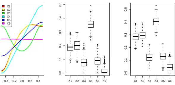
The plot function for "tgp" objects now provides a variety of ways to visualize the results of a sensitivity analysis. This capability is accessed by specifying layout = "sens" in the standard plot command. By default, the mean posterior main effects are plotted next to boxplot summaries of the posterior sample for eachSj andTj index, as in Figure5. The code used to create the figure is as follows.

R> plot(sf, layout = "sens", legendloc = "topleft")

A further note on the role played by nn.lhs: As always, the quality of the regression model estimate depends on the length of the MCMC. But now, the quality of sensitivity analysis is directly influenced by the size of the LHS used for integral approximation; as with any Monte Carlo integration scheme, the sample size (i.e.,nn.lhs) must increase with the dimensionality of the problem. In particular, it can be seen in the estimation procedure described above that the total sensitivity indices (theTj’s) are not forced to be non-negative. If negative values

0.0 0.4 0.8 −0.20 −0.10 0.00 0.05 0.10 X1 0.0 0.4 0.8 −0.20 −0.10 0.00 0.05 0.10 X2 response 0.0 0.4 0.8 −0.05 0.00 0.05 0.10 X3 response 0.0 0.6 −0.2 −0.1 0.0 0.1 0.2 X4 response 0.0 0.4 0.8 −0.10 −0.05 0.00 0.05 0.10 X5 response 0.0 0.4 0.8 −0.02 0.00 0.02 0.04 X6 response

Main effects: mean and 90 percent interval

Figure 6: Friedman function main effects, with posterior 90% intervals.

● ● ● ● ● ● ● ● ● ● ● ● ● ● ● ● ● ● ● ● ● ● ● ● ● ● ● ● ● ● ● ● ● ● ● ● ● ● ● ● ● ● ● ● ● ● ● ● ● ● ● X1 X2 X3 X4 X5 X6 0.0 0.1 0.2 0.3 0.4 0.5

1st order Sensitivity Indices

input variables ● ● ● ● ● ● ●●● ● ● ● ● ● ● ● ● ● ● ● ● ● ● X1 X2 X3 X4 X5 X6 0.0 0.1 0.2 0.3 0.4 0.5

Total Effect Sensitivity Indices

input variables

Figure 7: Sensitivity indices for the Friedman function.

occur it is necessary to increase nn.lhs. In any case, the plot method changes any of the negative values to zero for purposes of illustration.

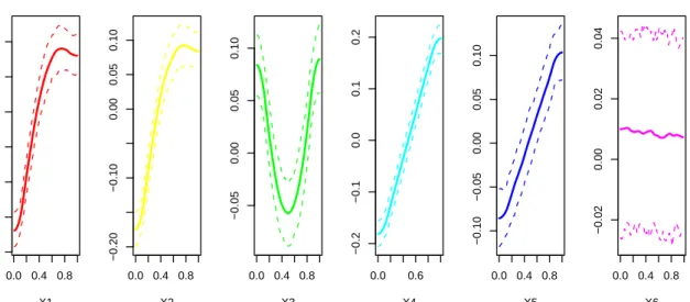
Themaineffargument can be used to plot either selected main effects (Figure6), or just the

sensitivity indices (Figure7).

R> plot(sf, layout = "sens", maineff = t(1:6)) R> plot(sf, layout = "sens", maineff = FALSE)

Note that the posterior intervals shown in these plots represent uncertainty about both the function response and the integration estimates; this full quantification of uncertainty is not presently available in any alternative SA procedures. These plots may be compared to what

we know about the Friedman function (refer to Equation 5) to evaluate the analysis. The main effects correspond to what we would expect: sine waves forx1 andx2, a parabola forx3,

and linear effects forx4 and x5. The sensitivity indices showx1 and x2 contributing roughly

equivalent amounts of variation, while x4 is relatively more influential than x5. Full effect

sensitivity indices forx3,x4, and x5 are roughly the same as the first order indices, but (due

to the interaction in the Friedman function) the sensitivity indices for the total effect of x1

and x2 are significantly larger than the corresponding first order indices. Finally, our SA is

able to determine thatx6 is unrelated to the response.

This analysis assumes the default uncertainty distribution, which is uniform over the range of input data. In other scenarios, it is useful to specify an informativeu(x). In thesensfunction, properties of u are defined through the rect, shape, and mode arguments. To guarantee integrability of our indices, we have restricted ourselves to bounded uncertainty distributions. Hence, rect defines these bounds. In particular, this defines the domain from which the LHSs are to be taken. We then use independent scaled beta distributions, parameterized by

theshapeparameter and distributionmode, to define an informative uncertainty distribution

over this domain.

As an example of sensitivity analysis under an informative uncertainty distribution, consider

theairquality data available with the base distribution of R. This data set contains daily

readings of mean ozone in parts per billion (Ozone), solar radiation (Solar.R), wind speed (Wind), and maximum temperature (Temp) for New York City, between May 1 and Septem-ber 30, 1973. Suppose that we are interested in the sensitivity of air quality to natural changes

inSolar.R,Wind, andTemp. For convenience, we will build our uncertainty distribution while

assuming independence between these inputs. Hence, for each variable, the input uncertainty distribution will be a scaled beta withshape = 2, andmode equal to the data mean.

R> X <- airquality[, 2:4] R> Z <- airquality$Ozone

R> rect <- t(apply(X, 2, range, na.rm = TRUE)) R> mode <- apply(X, 2, mean, na.rm = TRUE) R> shape <- rep(2, 3)

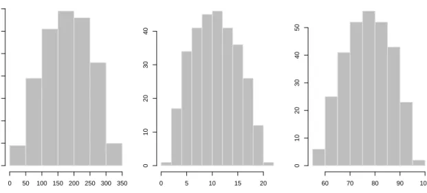
LHS samples from the uncertainty distribution are shown in Figure8, obtained as follows. R> Udraw <- lhs(300, rect = rect, mode = mode, shape = shape)

R> par(mfrow = c(1, 3), mar = c(4, 2, 4, 2))

R> for(i in 1:3) hist(Udraw[, i], breaks = 10, xlab = names(X)[i], + main = "", ylab = "", border = grey(0.9), col = 8)

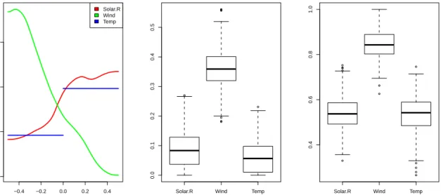
Due to missing data (discarded in the current version oftgp), we suppress warnings for the sensitivity analysis. We shall use the defaultmodel = btgp.

R> s.air <- suppressWarnings(sens(X = X, Z = Z, nn.lhs = 300, + rect = rect, shape = shape, mode = mode, verb = 0)) Figure9 shows the results from this analysis.

Solar.R 0 50 100 150 200 250 300 350 0 10 20 30 40 50 60 70 Wind 0 5 10 15 20 0 10 20 30 40 Temp 60 70 80 90 100 0 10 20 30 40 50

Figure 8: A sample from the marginal uncertainty distribution for the airquality data.

−0.4 −0.2 0.0 0.2 0.4 −0.15 −0.10 −0.05 0.00 0.05 0.10 Main Effects scaled input response Solar.R Wind Temp ● ● ● ● ● ● ● ●

Solar.R Wind Temp

0.0 0.1 0.2 0.3 0.4 0.5

1st order Sensitivity Indices

input variables ● ● ● ● ● ● ● ● ●

Solar.R Wind Temp

0.2

0.4

0.6

0.8

Total Effect Sensitivity Indices

input variables

Figure 9: Sensitivity of NYC airquality to natural variation in wind, sun, and temperature. Through use of thepredictmethod for"tgp"objects, it is possible to quickly re-analyze with respect to a new uncertainty distribution without running new MCMC. We can, for example, look at sensitivity for air quality on only low-wind days. We thus alter the uncertainty distribution (assuming that things remain the same for the other variables)

R> rect[2, ] <- c(0, 5) R> mode[2] <- 2

R> shape[2] <- 2

and build a set of parameterssens.p with the sensfunction by setting model = NULL. R> sens.p <- suppressWarnings(sens(X = X, Z = Z, nn.lhs = 300,

−0.4 −0.2 0.0 0.2 0.4 0.00 0.05 0.10 0.15 0.20 0.25 Main Effects scaled input response Solar.R Wind Temp ● ● ● ● ● ● ● ● ● ● ● ● ● ● ● ● ● ● ● ● ● ● ● ● ● ● ● ● ● ● ● ● ● ● ● ●

Solar.R Wind Temp

0.0 0.1 0.2 0.3 0.4 0.5 0.6

1st order Sensitivity Indices

input variables ● ● ● ● ● ● ● ● ● ● ● ● ● ● ● ● ● ●

Solar.R Wind Temp

0.0 0.2 0.4 0.6 0.8 1.0

Total Effect Sensitivity Indices

input variables

Figure 10: Air quality sensitivity on low-wind days.

−0.4 −0.2 0.0 0.2 0.4 −0.2 −0.1 0.0 0.1 Main Effects scaled input response Solar.R Wind Temp ● ● ● ● ● ● ● ●

Solar.R Wind Temp

0.0 0.1 0.2 0.3 0.4 0.5

1st order Sensitivity Indices

input variables ● ● ● ● ● ● ● ● ● ● ● ●

Solar.R Wind Temp

0.4

0.6

0.8

1.0

Total Effect Sensitivity Indices

input variables

Figure 11: Sensitivity of NYC airquality to natural variation in wind, sun, and a binary temperature variable (for a threshold of 79 degrees).

Figures9and10both show total effect indices which are much larger than the respective first order sensitivities. Figure10 was obtained as follows.

R> s.air2 <- predict(s.air, BTE = c(1, 1000, 1), sens.p = sens.p, verb = 0) R> plot(s.air2, layout = "sens")

As one would expect, the effect on airquality is manifest largely through an interaction between variables.

Finally, it is also possible to perform SA with binary covariates, included in the regression model as described in Section 1. In this case, the uncertainty distribution is naturally

charac-terized by a Bernoulli density. Settingshape[i] = 0informs sensthat the relevant variable is binary (perhaps encoding a categorical input as in Section 2), and that the Bernoulli uncertainty distribution should be used. In this case, the mode[i] parameter dictates the probability parameter for the Bernoulli, and we must have rect[i,] = c(0,1). As an ex-ample, we re-analyze the original air quality data with temperature included as an indicator variable (set to one if temperature>79, the median, and zero otherwise).

R> X$Temp[X$Temp > 70] <- 1 R> X$Temp[X$Temp > 1] <- 0

R> rect <- t(apply(X, 2, range, na.rm = TRUE)) R> mode <- apply(X, 2, mean, na.rm = TRUE) R> shape <- c(2, 2, 0)

R> s.air <- suppressWarnings(sens(X = X, Z = Z, nn.lhs = 300,

+ rect = rect, shape = shape, mode = mode, verb = 0, basemax = 2)) Figure11 shows the results from this analysis.

R> plot(s.air, layout = "sens")

4. Statistical search for optimization

There has been considerable recent interest in the use of statistically generated search patterns (i.e., locations of relatively likely optima) for optimization. A popular approach is to estimate a statistical (surrogate) model, and use it to design a set of well-chosen canidates for further evaluation by a direct optimization routine. Such statistically designed search patterns can be used either to direct the optimization completely (e.g.,Joneset al.1998;Regis and Shoemaker 2007) or to work in hybrid with local pattern search optimization (as inTaddyet al.2009). An bonus feature of the statistical surrogate approach is that it may be used to tackle problems of optimization under uncertainty, wherein the function being optimized is observed with noise. In this case the search is for input configurations which optimize the response with high probability. Direct-search methods would not apply in this scenario without modification. However, a sensible hybrid could involve inverting the relationship between the two approaches so that direct-search is used on deterministic predictive surfaces from the statistical surrogate model. This search can be used to find promising candidates to compliment space-filling ones at which some statistical improvement criterion is evaluated.

Towards situatingtgpas a promising statistical surrogate model for optimization (in both con-texts) the approach developed byTaddyet al.(2009) has been implemented to produce a list of input locations that is ordered by a measure of the potential for new optima. The procedure uses samples from the posterior predictive distribution of treed GP regression models to esti-mate improvement statistics and build an ordered list of search locations which maximize ex-pected improvement. The single location improvement is definedI(x) = max{fmin−f(x),0}, wherefmin is the minimum evaluated response in the search (refer toSchonlau et al. (1998)

for extensive discussion on general improvement statistics and initial vignette (Gramacy 2007) for details of a base implementation in tgp). Thus, a high improvement corresponds to an input location that is expected to be much lower than the current minimum. The criterion

is easily changed to a search for maximum values through negation of the response. The im-provement is always non-negative, as points which do not turn out to be new minimum points still provide valuable information about the output surface. Thus, in the expectation, candi-date locations will be rewarded for high response uncertainty (indicating a poorly explored region of the input space), as well as for low mean predicted response. Our tgp generated search pattern will consist ofmlocations that recursively maximize (over a discrete candidate set) a sequential version of the expected multi-location improvement developed bySchonlau

et al.(1998), defined as E[Ig(x1, . . . ,xm)] where

Ig(x1, . . . ,xm) = (max{(fmin−f(x1)), . . . ,(fmin−f(xm)),0})g. (6)

Increasing g ∈ {0,1,2,3, . . .} increases the global scope of the criteria by rewarding in the expectation extra variability at x. For example, g = 0 leads to E[I0(x)] = P(I(x) > 0) (assuming the convention 00= 0), g= 1 yields the standard statistic, andg= 2 explicitly re-wards the improvement variance sinceE[I2_{(x)] =VAR[I(x)] +E[I(x)]}2_{. For further discussion}

on the role ofg, see Schonlauet al. (1998) .

Finding the maximum expectation of (6) is practically impossible for the full posterior dis-tribution of Ig(x1, . . . ,xm), and would require conditioning on a single fit for the model

parameters (for example, static imputation of predictive GP means can be used to recursively build the improvement set (Ginsbourgeret al. 2009)). However, tgp just seeks to maximize over a discrete list of predictive locations. In fact, the default is to return an ordering for the entire XX matrix, thus defining a ranking of predictive locations by order of decreasing expected improvement. There is no restriction on the form for XX.1 The structure of this scheme will dictate the form forXX. If it is the case that we seek simply to explore the input space and map a list of potential locations for improvement, using LHS to choose XX will suffice.

The discretization of decision space allows for a fast iterative solution to the optimization of

E[Ig(x1, . . . ,xm)]. This begins with evaluation of the simple improvementIg(˜xi) over ˜xi∈X˜

at each ofT =BTE[2] - BTE[1]MCMC iterations (each corresponding to a single posterior realization of tgp parameters and predicted response after burn-in) to obtain the posterior sample I =      Ig(˜x1)1 . . . Ig(˜xm)1 .. . Ig(˜x1)T . . . Ig(˜xm)T      .

Recall that intgpparlance, and as input to the b*functions: ˜X≡XX.

We then proceed iteratively to build an ordered collection of m locations according to an iteratively refined improvement: Designate x1 = argmax_˜x∈_X˜E[Ig(˜x)], and for j = 2, . . . , m,

given thatx1, . . . ,xj−1 are already included in the collection, the next member is

xj = argmax_x˜∈_X˜E[max{Ig(x1, . . . ,xj−1), Ig(˜x)}]

= argmax_x˜∈X˜E[(max{(fmin−f(x1)), . . . ,(fmin−f(xj−1)),(fmin−f(˜x)),0})g]

= argmax_x˜∈X˜E[Ig(x1, . . . ,xj−1,x˜)].

1

A full optimization routine would require that the search pattern is placed within an algorithm iterating towards convergence, as inTaddy et al. (2009). However, we concentrate here on the statistical problem of choosing the next samples optimally. We shall touch on issues of convergence in Section4.2where we describe a skeleton scheme for optimization extendingR’s internaloptimfunctionality.

Thus, after each jth additional point is added to the set, we have the maximum expected

j-location improvement conditional on the first j−1 locations. This is not necessarily the unconditionally maximal expected j-location improvement; instead, point xj is the location

which will cause the greatest increase in expected improvement over the given (j−1)-location expected improvement.

The posterior sample I acts as a discrete approximation to the true posterior distribution for improvement at locations within the candidate set XX. Based upon this approximation, iterative selection of the point set is possible without any re-fitting of thetgpmodel. Condi-tional on the inclusion of ˜xi1, . . . ,x˜il−1 in the collection, a posterior sample of the l-location improvement statistics is calculated as

Il =      Ig(˜xi1, . . . ,x˜il−1,˜x1)1 . . . I g_(˜x i1, . . . ,x˜il−1,x˜m)1 .. . Ig(˜xi1, . . . ,x˜il−1,x˜1)T . . . I g_(˜x i1, . . . ,x˜il−1,x˜m)T      ,

where the element in thetth row andjth column of this matrix is calculated as max{Ig(˜xi1,

. . . ,x˜il−1)t,I

g_(˜x

j)t}and thelth location included in the collection corresponds to the column

of this matrix with maximum average. Since the multi-location improvement is always at least as high as the improvement at any subset of those locations, the same points will not be chosen twice for inclusion. In practice, very few iterations (about 10% of the total candidate size under the default inference and regression model(s)) through this ordering process can be performed before the iteratively updated improvement statistics become essentially zero. Increasing the number of MCMC iterations (BTE[2] - BTE[1]) can mitigate this to a large extent.2 We refer the reader to Taddy et al. (2009) for further details on this approach to multi-location improvement search.

4.1. A simple example

We shall use the Rosenbrock function to illustrate the production of an ordered collection of (possible) adaptive samples to maximize the expected improvement withintgp. Specifically, the two dimensional Rosenbrock function is defined as

R> rosenbrock <- function(x) { + x <- matrix(x, ncol = 2)

+ 100 * (x[, 1]^2 - x[, 2])^2 + (x[, 1] - 1)^2 + }

and we shall bound the search space for adaptive samples to the rectangle: −1≤xi ≤5 for i= 1,2. The single global minimum of the Rosenbrock function is at (1,1).

R> rosenbrock(c(1, 1))

[1] 0

This function involves a long steep valley with a gradually sloping floor, and is considered to be a difficult problem for local optimization routines.

2

Once a zero (maximal) iterative improvement is attained the rest of the ranking is essentially arbitrary, at which pointtgpcuts off the process prematurely.

We begin by drawing an LHS of 40 input locations within the bounding rectangle, and eval-uating the function at these locations.

R> rect <- cbind(c(-1, -1), c(5, 5)) R> X <- lhs(40, rect)

R> Z <- rosenbrock(X)

We will fit abgpmodel to this data to predict the Rosenbrock response at unobserved (can-didate) input locations in XX. The improv argument may be used to obtain an ordered list of places where we should be looking for new minima. In particular, specifying improv =

c(1,10) will return the 10 locations which maximize the iterative multi-location expected

improvement function, withg= 1 (i.e., Equation6). Note that improv = TRUE is also possi-ble, in which casegdefaults to one and the entire list of locations is ranked. Our candidate set is just a space filling LHS design. In other situations, it may be useful to build an informative LHS design (i.e., to specifyshape and mode arguments for the lhsfunction) to reflect what is already known about the location of optima.

R> XX <- lhs(200, rect)

R> rfit <- bgp(X, Z, XX, improv = c(1, 10), verb = 0)

Upon return, the"tgp"-class object rfit includes the matriximprov, which is a list of the expected single location improvement for the 200XX locations, and the top 10 ranks. Note that theranks for those points which are not included in the top 10 are set to nrow(XX) =

200. Here are the top 10:

R> cbind(rfit$improv, XX)[rfit$improv$rank <= 10, ] improv rank 1 2 4 0.0006420693 4 1.41243478 2.15174711 12 0.0006589185 8 0.04339625 0.09489153 15 0.0006277068 7 -0.25358237 0.14341675 20 0.0006525640 5 1.31313812 1.87566387 21 0.0006212942 9 1.60593438 2.38150541 119 0.0006140362 6 1.61718015 2.39090831 154 0.0006927117 1 0.13792447 -0.01324855 164 0.0006110359 10 0.05915976 -0.27341950 182 0.0006233682 3 2.22019217 4.76719757 200 0.0006598981 2 2.04231115 3.99968412

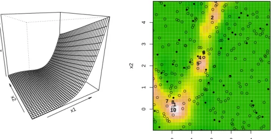
This iterative algorithm may produce ranks that differ significantly from a straightforward ordering of expected improvement. This leads to a list that better explores the input space, since the expected improvement is naturally balanced against a desire to search the domain. We plot the results with the usual function, by settingas = "improv", in Figure 12.

R> plot(rfit, as = "improv")

The banana-shaped region of higher expected improvement corresponds to the true valley floor for the Rosenbrock function, indicating the thatbgpmodel is doing a good job of prediction.

x1 x2 z z mean 0 1 2 3 4 0 1 2 3 4 z Improv stats (g=1) x1 x2 ● ● ● ● ● ● ● ● ● ● ● ● ● ● ● ● ● ● ● ● ● ● ● ● ● ● ● ● ● ● ● ● ● ● ● ● ● ● ● ● ● ● ● ● ● ● ● ● ● ● ● ● ● ● ● ● ● ● ● ● ● ● ● ● ● ● ● ● ● ● ● ● ● ● ● ● ● ● ● ● ● ● ● ● ● ● ● ● ● ● ● ● ● ● ● ● ● ● ● ● ● ● ● ● ● ● ● ● ● ● ● ● ● ● ● ● ● ● ● ● ● ● ● ● ● ● ● ● ● ● ● ● ● ● ● ● ● ● ● ● ● ● ● ● ● ● ● ● ● ● ● ● ● ● ● ● ● ● ● ● ● ● ● ● ● ● ● ● ● ● ● ● ● ● ● ● ● ● ● ● ● ● ● ● ● ● ● ● ● ● ● ● ● ● ● ● ● ● ● ● ● ● ● ● ● ● ● ● ● ● ● ● ● ● ● ● ● ● ● ● ● ● ● ● ● ● ● ● ● ● ● ● ● ● ● ● ● ● ● ● 4 8 7 5 96 1 10 3 2

Figure 12: The left panel shows the mean predicted Rosenbrock function response, and on

theright we have expected single location improvement with the top 10 points (labelled by

rank) plotted on top.

Also, we note that the ordered input points are well dispersed throughout the valley—a very desirable property for adaptive sampling candidates.

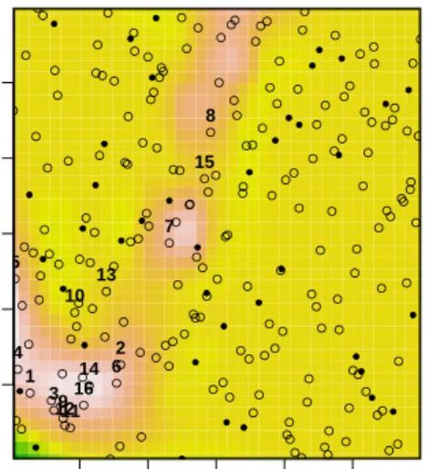
It is straightforward, with thepredict method for "tgp" objects, to obtain a new ordering for the more globalg = 5(or any new g).

R> rfit2 <- predict(rfit, XX = XX, BTE = c(1, 1000, 1), improv = c(5, 20), + verb = 0)

R> plot(rfit2, layout = "as", as = "improv")

Figure 13 shows the resulting plot, which indicates a more diffuse expected improvement surface and a substantially different point ordering. In practice, we have found that g = 2

provides a good compromise between local and global search. 4.2. A skeleton optimization scheme

The capabilities outlined above are useful in their own right, as a search list or candidate set ranked by expected improvement gain provides concrete information about potential optima. However, a full optimization framework requires that the production of these sets of search locations are nested within an iterative search scheme. The approach taken by Taddy et al. (2009) achieves this by taking thetgpgenerated sets of locations and using them to augment a local optimization search algorithm. In this way, the authors are able to achieve robust solutions which balance the convergence properties of the local methods with the global scope provided by tgp. Indeed, any optimization routine capable of evaluating points provided by an outside source could benefit from a tgpgenerated list of search locations.

In the absence of this sort of formal hybrid search algorithm, it is still possible to devise robust optimization algorithms based aroundtgp. A basic algorithm is as follows: first, use a

0 1 2 3 4 0 1 2 3 4 z Improv stats (g=5) x1 x2 ● ● ● ● ● ● ● ● ● ● ● ● ● ● ● ● ● ● ● ● ● ● ● ● ● ● ● ● ● ● ● ● ● ● ● ● ● ● ● ● ● ● ● ● ● ● ● ● ● ● ● ● ● ● ● ● ● ● ● ● ● ● ● ● ● ● ● ● ● ● ● ● ● ● ● ● ● ● ● ● ● ● ● ● ● ● ● ● ● ● ● ● ● ● ● ● ● ● ● ● ● ● ● ● ● ● ● ● ● ● ● ● ● ● ● ● ● ● ● ● ● ● ● ● ● ● ● ● ● ● ● ● ● ● ● ● ● ● ● ● ● ● ● ● ● ● ● ● ● ● ● ● ● ● ● ● ● ● ● ● ● ● ● ● ● ● ● ● ● ● ● ● ● ● ● ● ● ● ● ● ● ● ● ● ● ● ● ● ● ● ● ● ● ● ● ● ● ● ● ● ● ● ● ● ● ● ● ● ● ● ● ● ● ● ● ● ● ● ● ● ● ● ● ● ● ● ● ● ● ● ● ● ● ● ● ● ● ● ● ● 4 7 1 3 11 9 12 6 2 5 8 14 16 15 10 13

Figure 13: The expected improvement surface and top 20 ordered locations, for g = 5.

LHS to explore the input space (see thelhsfunction included intgp). Repeatedly fit one of theb* models withimprov != FALSEto the evaluated iterates to produce a search set, then evaluate the objective function over this search set, as described earlier. Then evaluate the objective function over the highest ranked locations in the search set. Continue until you are confident that the search has narrowed to a neighborhood around the true optimum (a good indicator of this is when all of the top-ranked points are in the same area). At this point, the optimization may be completed byoptim, R’s general purpose local optimization algorithm in order to guarentee convergence. The optim routine may be initialized to the best input location (i.e., corresponding the most optimal function evaluation) found thus far bytgp. Note that this approach is actually an extreme version of a template proposed by Taddy

et al.(2009) where the influence of global (i.e., tgp) search is downweighted over time rather than cut off. In either case, a drawback to such approaches is that they do not apply when the function being optimized is deterministic. An alternative scheme is to employ bothtgp

search and a local optimization at each iteration. The idea is that a mix of local and global information is provided throughout the entire optimization, but with an added twist. Rather than applyoptim on the stochastic function directly, which would not converge due to the noise, it can be applied on a deterministic (MAP) kriging surface provided by tgp. The local optima obtained can be used to augment the candidate set of locations where the improvement statistic is gathered—which would otherwise be simple LHS. That way the search pattern produced on output is likely to have a candidate with high improvement.

To fix ideas, and for the sake of demonstration, the tgppackage includes a skeleton function for performing a single iteration in the derivative-free optimization of noisy black-box func-tions. The function is called optim.step.tgp, and the name is intended to emphasize that it performs a single step in an optimization by trading off local optim-based search of tgp

predictive (kriging surrogate) surfaces, with the expected posterior improvement. In other words, it is loosely based on some the techniques alluded to above, but is designed to be aug-mented/adjusted as needed. GivenN pairs of inputs and responses (X,Z),optim.step.tgp

suggests new points at which the function being optimized should be evaluated. It also returns information that can be used to assess convergence. An outline follows.

Theoptim.step.tgpfunction begins by constructing a set of candidate locations, either as a

space filling LHS over the input space (the default) or from a treedD-optimal design, based on a previously obtained"tgp"-class model. R’soptimcommand is used on the MAP predictive surface contained within the object to obtain an estimate of the current best guessx-location of the optimal solution. A standalone subroutine called optim.ptgpf is provided for this specific task, to be used within optim.step.tgp or otherwise. Within optim.step.tgp,

optim.ptgpfis initialized with the data location currently predicted to be the best guess of

the minimum. The optimalx-location found is then added into the set of candidates as it is likely that the expected improvement would be high there.

Then, a new"tgp"-class object is obtained by applying ab*function to (X,Z) whilst sampling from the posterior distribution of the improvement statistic. The best one, two, or several locations with highest improvement ranks are suggested for addition into the design. The values of the maximum improvement statistic are also returned in order to track progress in future iterations. The "tgp"-class object returned is used to construct candidates and initialize theoptim.ptgpf function in future rounds.

To illustrate, consider the 2-d exponential data from the initial vignette (Gramacy 2007) as our noisy functionf.

R> f <- function(x) exp2d.Z(x)$Z

Recall that this data is characterized by a mean value of

f(x) =x1exp(−x21−x22)

which is observed with a small amount of Gaussian noise (with sd = 0.001). Elementary calculus gives that the minimum off is obtained at x= (−p1/2,0).

The optim.step.tgp function requires that the search domain be defined by a bounding

rectangle, and we require an initial design to start things off. Here we shall use [−2,6]2 _with

an LHS design therein.

R> rect <- rbind(c(-2, 6), c(-2, 6)) R> X <- lhs(20, rect)

R> Z <- f(X)

The following code proceeds with several rounds of sequential design towards finding the minimum of f.

R> out <- progress <- NULL R> for(i in 1:20) {

+ out <- optim.step.tgp(f, X = X, Z = Z, rect = rect, prev = out, verb = 0) + X <- rbind(X, out$X)

+ Z <- c(Z, f(out$X))

+ progress <- rbind(progress, out$progress) + }

5 10 15 20 −2.0 −1.5 −1.0 −0.5 0.0 0.5 1.0 x progress rounds x[,1:2] x1 x2 5 10 15 20 −10 −8 −6 −4

max log improv

rounds

max log(impro

v)

Figure 14: Progress in iterations of optim.step.tgp shown by tracking the x-locations of the best guess of the minimum (left) and the logarithm of the maximum of the improvement statistics at the candidate locations (right)

The progress can be tracked through the rows of a data.frame, as constructed above,

containing a listing of the input location of the current best guess of the minimum for each round, together with the value of the objective at that point, as well as the maximum of the improvement statistic. In addition to printing this data to the screen, plots such as the ones in Figure 14 can be valuable for assessing convergence. The plots were obtained as follows. R> par(mfrow = c(1, 2))

R> matplot(progress[, 1:2], main = "x progress", xlab = "rounds", + ylab = "x[,1:2]", type = "l", lwd = 2)

R> legend("topright", c("x1", "x2"), lwd = 2, col = 1:2, lty = 1:2) R> plot(log(progress$improv), type = "l", main = "max log improv", + xlab = "rounds", ylab = "max log(improv)")

As can be seen in the figure, the final iteration gives an x-value that is very close to the correct result, and is (in some loose sense) close to convergence.

R> out$progress[1:2]

x1 x2

1 -0.713727 -0.003497789

As mentioned above, if it is known that the function evaluations are deterministic then, at any time, R’s optim routine can be invoked—perhaps initialized by the x-location in

out$progress—and convergence to a local optimum thus guaranteed. Otherwise, the

used in each round, above, (T = BTE[2] - BTE[1]) tends to infinity. Such arguments to theb*functions can be set via the ellipses (...) arguments to optim.step.tgp.3 A heuris-tic stopping criterion can be based on the maximum improvement statisheuris-tic obtained in each round as long as the candidate locations become dense in the region asT → ∞. This can be adjusted by increasing theNNargument tooptim.step.tgp.

The internal use ofoptimwithinoptim.step.tgp on the posterior predictive (kriging surro-gate) surface viaoptim.ptgpf may proceed with any of the usual method arguments. I.e., R> formals(optim)$method

c("Nelder-Mead", "BFGS", "CG", "L-BFGS-B", "SANN")

however the default ordering is switched inoptim.ptgpf and includes one extra method. R> formals(optim.ptgpf)$method

c("L-BFGS-B", "Nelder-Mead", "BFGS", "CG", "SANN", "optimize")

Placing"L-BFGS-B"in the default position is sensible since this method enforces a rectangle of constraints as specified by rect. This guarentees that the additional candidate found by

optim.ptfpf will be valid. However, the other optim methods generally work well despite

that they do not enforce this constraint. The final method, "optimize", applies only when the inputs tofare 1-d. In this case, the documentation foroptimsuggests using theoptimize

function instead.

5. Importance tempering

It is well-known that MCMC inference in Bayesian treed methods suffers from poor mixing. For example Chipman et al. (1998,2002) recommend periodically restarting the MCMC to avoid chains becoming stuck in local modes of the posterior distribution (particularly in tree space). The treed GP models are or no exception, although it is worth remarking that using flexible GP models at the leaves of the tree typically results in shallower trees, and thus less pathalogical mixing in tree space. Version 1.x provided some crude tools to help mitigate the effects of poor mixing in tree space. For example, the R argument to the b* functions facilitates the restarts suggested by Chipman et al.

A modern Monte Carlo technique for dealing with poor mixing in Markov chain methods is to employtemperingto flatten the peaks and raise the troughs in the posterior distribution so that movements between modes is more fluid. One such method, calledsimulated tempering

(ST) (Geyer and Thompson 1995), is essentially the MCMC analogue of the popular simulated annealing algorithm for optimization. The ST algorithm helps obtain samples from a multi-modal densityπ(θ) where standard methods, such as Metropolis–Hastings (MH) (Metropolis

et al.1953;Hastings 1970) and Gibbs Sampling (GS) (Geman and Geman 1984), fail. 3_{This runs contrary to how the ellipses are used by}

optimin order to specify static arguments tof. If setting static arguments tofis required withinoptim.step.tgp, then they must be set in advance by adjusting the default arguments viaformals.