Solving the Quadratic Assignment Problem with
Cooperative Parallel Extremal Optimization
Danny Munera, Daniel Diaz, Salvador Abreu
To cite this version:
Danny Munera, Daniel Diaz, Salvador Abreu. Solving the Quadratic Assignment Problem
with Cooperative Parallel Extremal Optimization. 16th European Conference on Evolutionary
Computation in Combinatorial Optimization, EvoCOP 2016, Mar 2016, Porto, Portugal. 2016,
<
10.1007/978-3-319-30698-8 17
>
.
<
hal-01332524
>
HAL Id: hal-01332524
https://hal.archives-ouvertes.fr/hal-01332524
Submitted on 16 Jun 2016
HAL
is a multi-disciplinary open access
archive for the deposit and dissemination of
sci-entific research documents, whether they are
pub-lished or not.
The documents may come from
teaching and research institutions in France or
abroad, or from public or private research centers.
L’archive ouverte pluridisciplinaire
HAL
, est
destin´
ee au d´
epˆ
ot et `
a la diffusion de documents
scientifiques de niveau recherche, publi´
es ou non,
´
emanant des ´
etablissements d’enseignement et de
recherche fran¸
cais ou ´
etrangers, des laboratoires
publics ou priv´
es.
Solving the Quadratic Assignment Problem with
Cooperative Parallel Extremal Optimization
Danny Munera1, Daniel Diaz1and Salvador Abreu2,1
1
University of Paris 1-Sorbonne/CRI, France
2 Universidade de ´Evora/LISP, Portugal
Abstract. Several real-life applications can be stated in terms of the
Quadratic Assignment Problem. Finding an optimal assignment is com-putationally very difficult, for many useful instances. We address this problem using a local search technique, based on Extremal Optimiza-tion and present experimental evidence that this approach is competi-tive. Moreover, cooperative parallel versions of our solver improve per-formance so much that large and hard instances can be solved quickly.
Keywords: QAP, extremal optimization, heuristics, parallelism, cooperation
1
Introduction
The Quadratic Assignment Problem (QAP) was introduced in 1957 by Koop-mans and Beckmann [1] as a model of a facilities location problem. This problem consists in assigning a set ofnfacilities to a set ofnspecific locations minimizing the cost associated with theflows of items among facilities and thedistance be-tween them. This combinatorial optimization problem has many other real-life applications: scheduling, electronic chipset layout and wiring, process commu-nications, turbine runner balancing, data center network topology, to cite but a few [2,3]. Unfortunately this problem is known to be NP-hard and finding efficient algorithms to solve it has attracted a lot of research in recent years.
Exact (or complete) methods like dynamic programming, cutting plane tech-niques and branch & bound procedures have been successfully applied to medium-size QAP instances but cannot solve larger instances (e.g. when n > 20). To tackle these problems, one must resort to incomplete methods which are de-signed to quickly provide good, albeit sub-optimal, solutions. This is the case of approximation algorithms, i.e. algorithms running in polynomial time yet able to guarantee solutions within a constant factor of the optimum. Unfortunately, it is known that there is no-approximation algorithm for the QAP [4]. Another class of incomplete methods is provided by meta-heuristics. Since 1990 several meta-heuristics have been successfully applied to the QAP: tabu search, simu-lated annealing, genetic algorithms, GRASP, ant-colonies [3]. The current trend is to specialize existing heuristics, to compose different meta-heuristics (hybrid procedures) and to use parallelism.
In this paper we propose EO-QAP: an Extremal Optimization (EO) proce-dure for QAP. EO is a nature-inspired general-purpose meta-heuristics to solve combinatorial optimization problems [5]. This local search procedure, a priori, has several advantages: it is easy to implement, it does not get confounded by local minima and takes only one adjustable parameter. We experimentally demonstrate that EO-QAP performs well on the set of QAPLIB benchmark in-stances. It is, however, known that it is difficult with EO to have fine control on the trade-off between search intensification anddiversification: some strate-gies have been proposed to overcome this limitation [6], but they entail a more complex tuning process. In this paper we put forth two other approaches which contribute to a more effective handling of QAP using EO: firstly, we propose a simple extension to the original EO which allows the user to have more control over the stochastic behavior of the algorithm. Secondly, we propose to use coop-erative parallelism to promote more intensification and/or diversification. Our implementation uses a parallel framework [7] written in X10 [8,9]. We show that the cooperative parallel version behaves very well on the hardest instances.
The rest of the paper is organized as follows. Section 2 discusses QAP and provides the necessary background. Section 3 presents our EO algorithm for QAP and proposes an extension to the original EO. Several experimental results are laid out and discussed in section 4 and we conclude in Section 5.
2
Background
Before introducing the main object of this paper, we need to recall some back-ground topics: the Quadratic Assignment Problem (QAP), Extremal Optimiza-tion (EO) and Cooperative Parallel Local Search (CPLS).
2.1 QAP
Since its introduction in 1957, QAP has been widely studied and several surveys are available [10,2,11,3].
A QAP problem of sizenconsists of twon×nmatrices (aij) and (bij). Let
Π(n) be the set of all permutations of{1,2, . . . n}, the goal of QAP is to find a permutationπ∈Π(n) which minimizes the following objective function:
F(π) = n X i=1 n X j=1 aij·bπiπj (1)
For instance, in facility location problems, the a matrix represents inter-facility flows and b encodes the inter-location distances. In that context, both matrices are generally symmetric: ∀i,j aij = aji and bij = bji. However, in other settings the matrices can become asymmetric. Indeed, QAP can be used to model scheduling, chip placement and wiring on a circuit board, to design typewriter keyboards, for process communications, for turbine runner balancing among many other applications [2,12].
The computational difficulty of QAP stems form the fact that the objective function contains products of variables (hence the term quadratic) and in the fact that the theoretical search space of an instance of sizenis the set of all per-mutationsΠ(n) whose cardinality isn!. In 1976, Sahni and Gonzalez proved that QAP is NP-hard [4] (the famous traveling salesman problem can be formulated as a QAP). Moreover, the same authors proved that there is no-approximation algorithm for QAP (unless P=NP). In practice QAP is one of the most difficult combinatorial optimization problems with many real-life applications.
QAP can be (optimally) solved with exact methods like dynamic program-ming, cutting plane techniques and branch & bound algorithms (together with efficient lower bound methods). Constraint Programming does not work well on QAP and, surprisingly, SAT solvers have not been extensively used for QAP. However, general problems of medium size (e.g. n > 20) are out of reach for these methods (even if some particular larger instances can be solved). It is thus natural to use heuristics to solve QAP. In the last decades several meta-heuristics were successfully applied to QAP: tabu search, simulated annealing, genetic al-gorithms, GRASP, ant-colonies [13]. In this paper we propose to use Extremal Optimization to attack QAP problems.
2.2 Extremal Optimization
In 1999, Boettcher and Percus proposed the Extremal Optimization (EO) proce-dure [5,14,15] as a meta-heuristics to solve combinatorial optimization problems. EO is inspired by self-organizing processes often found in nature. It based on the concept ofSelf-Organized Criticality(SOC) initially proposed by Bak [16,17] and in particular by the Bak-Sneppen model of SOC [18]. In this model of bio-logical evolution, specieshave afitness ∈[0,1] (0 representing the worst degree of adaptation). At each iteration, the species with the worst fitness value is up-dated, i.e. its fitness is replaced by a new random value. This change also affects all other species connected to this “culprit” element and their fitness value also gets updated. This results in anextremal process which progressively eliminates the least fit species (or forces them to mutate). Repeating this process eventually leads to a state where all species have a good fitness value, i.e. a SOC. EO follows this line: it inspects the current configuration (assignment of variables), selects the worst variable (the one having the lowest fitness) and replaces its value by a random value. However, always selecting the worst variable can lead to a de-terministic behavior and the algorithm can stay blocked in a local minimum. To avoid this, the authors propose an extended algorithm which first ranks the variables in increasing order of fitness (the worst variable has thus a rankk= 1) and then resorts to a Probability Distribution Function(PDF) over the ranks k
in order to introduce uncertainty in the search process:
P(k) =k−τ (1≤k≤n) (2)
This power-law probability distribution takes a single parameterτ which is problem-dependent. Depending on the value ofτ, EO provides a wide variety of
search strategies from pure random walk (τ= 0) to deterministic (greedy) search (τ→ ∞). With an adequate value forτ, EO cannot be trapped in local minima since any variable is susceptible to mutate (even if the worst are privileged). This parameter can be tuned by the user. Moreover, the original paper proposes a default value depending onn:τ= 1 + ln1(n).
EO displays several a priori advantages: it is a simple meta-heuristic (it can be easily programmed), it is controlled by only one free parameter (a fine tuning of several parameters becomes quickly tedious) and it does not need to be aware about local minima. Nevertheless, EO has been successfully applied to large-scale optimization problems like graph bi-partitioning, graph coloring, Spin Glasses or the traveling salesman problem [14]. Boettcher and Percus point out, however, that depending on the problem,“a drawback of the EO method is that a general definition of fitness for the individual variables may prove ambiguous or even impossible” [19]. To overcome this, De Sousa and Ramos proposed an exten-sion called Generalized Extremal Optimization [20,21]. Zhou and al. proposed a variant called Continuous Extremal Optimization to deal with continuous opti-mization problems [22]. It has been also argued that one main issue with EO is that is does not provide a fine control of the intensification. Randall and Lewis propose some intensification strategies to improve EO [6]. We present two alter-natives to overcome this limitation: we propose a simple extension to improve the stochastic capabilities of EO and we show how cooperative parallelism can help to achieve intensification or diversification through communications.
2.3 Cooperative Parallel Local Search
Parallel local search methods have been proposed in the past [23,24,25]. In this article we are interested in multi-walk methods (also called multi-start) which consist in a concurrent exploration of the search space, either independently or cooperatively via communication between processes. TheIndependent Multi-Walks method (IW) [26] is the easiest to implement since the solver instances do not communicate with each other. However, the resulting gain tends to flatten when scaling over a hundred of processors [27], and can be improved upon. In the Cooperative Multi-Walks (CW) method [28], the solver instances exchange infor-mation (through communication), hoping to hasten the search process. However, implementing an efficient cooperative method is a very complex task: several choices have to be made about the communication which influence each other and which are problem-dependent [28].
We build on the framework for Cooperative Parallel Local Search (CPLS) proposed in [29,7]. This framework, available as an open source library in the X10 programming language, allows the programmer to tune the search process through an extensive set of parameters which, in the present version, statically condition the execution. CPLS augments the IW strategy with a tunable commu-nication mechanism, which allows for the cooperation between the multiple in-stances to seek either an intensification or diversification strategy for the search. At present, the tuning process is done manually: we have not yet experimented with parameter self-adaptation (still an experimental feature).
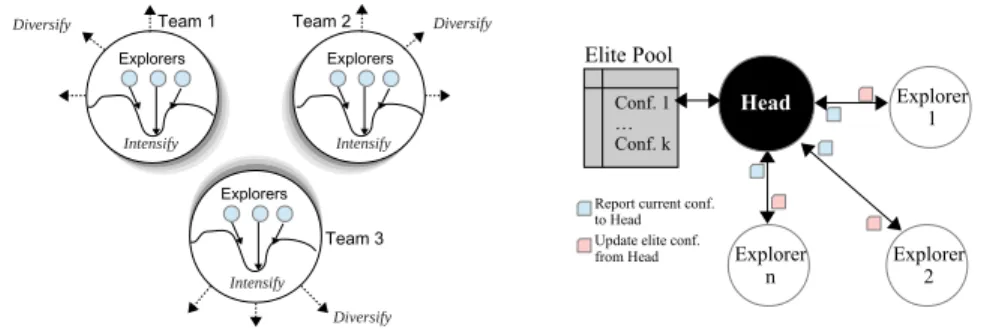
The basic component of CPLS is theexplorer node which consists in a local search solver instance. The point is to use all the available processing units by mapping eachexplorer node to a physical core. Explorer nodes are grouped into teams, of size N P T (see Figure 1). This parameter is directly related to the trade-off between intensification and diversification.N P T can take values from 1 to the maximum number of nodes (frequently linked to maximum number of available cores in the execution). When N P T is equal to 1, the framework coincides with the IW strategy, it is expected that each 1-node team be working on a different region of the search space, without seek parallel intensification.
WhenN P T is equal to the maximum number of nodes (creating only 1 team in
the execution), the framework has the maximum level of parallel intensification, but it is not possible to enable parallel diversification between teams.
Intensify Team 2 Diversify Explorers Intensify Explorers Intensify Explorers Diversify Diversify Team 1 Team 3 Explorer n Elite Pool Head Conf. 1 … Conf. k Report current conf. to Head Update elite conf. from Head
Explorer 1
Explorer 2
Fig. 1: CPLS framework structure
Each team seeks tointensify the search in the most promising neighborhood found by any of its members. The parameters which guide the intensification are the Report Interval (R) andUpdate Interval (U): every R iterations, each explorer node sends its current configuration and the associated cost to itshead node. The head node is the team member which collects and processes this in-formation, retaining the best configurations in an Elite Pool (EP) whose size |EP|is parametric. EveryU iterations, explorer nodes randomly retrieve a con-figuration from the EP, in the head node. An explorer node may adopt the configuration from theEP, if it is “better” than its own current configuration with a probabilitypAdopt. Simultaneously, the teams implement a mechanism to cooperativelydiversify the search, i.e. they try to extend the search to different regions of the search space.
Typically, each problem benefits from intensification and diversification on some level. Therefore, the tuning process of the CPLS parameters seeks to pro-vide the appropriate balance between the use of the intensification and diver-sification mechanisms, in hope of reaching better performance than the non-cooperative parallel solvers (e.g. Independent Multi-Walks). A detailed descrip-tion of this framework may be found in [7].
3
EO-QAP: an EO Procedure for QAP
3.1 General Procedure
Our EO-QAP algorithm starts from a random permutationπ∈Π(n), with an associated cost given byF(π). To ensure we only consider proper permutations, we only performswap operations on pairs of elements from any given one: this is how value assignment is classically implemented in permutation problems, thereby eschewing the costly explicitly encoding of anall-differentconstraint. We define the permutation resulting from swappingπi andπj:
πi↔j =µ|µi=πj, µj =πi, µk=πk ∀k6∈ {i, j} (3)
The neighborhood ofπi is the setN(πi) of the permutations obtained from
πby swappingπi with any another value. By extension, the neighborhood ofπ is the setN(π) of all permutations obtained by swapping any two values:
N(πi) ={πi↔j |1≤j≤n, j6=i} (4) N(π) = n [ i=1 N(πi) (5)
Most local search procedures (in particularhill climbing) would select, among all elements ofN(π),the best neighborµ, i.e. the one minimizing the next global cost function. By doing so, they have to deal with the problem of being trapped in a local minimum. Instead, EO defines afitnessvalueλifor each valueπi, with the understanding that a value with a low fitness is more likely to mutate, i.e. to get swapped. We define the fitness valueλi as the best possible improvement of the costF when moving to aπi’s neighbor.
λi = min
µ∈N(πi)
F(µ)−F(π) (6)
A negativeλthus represents an improvement of the cost. At each iteration, the n fitness values are evaluated and ranked, with rank k = 1 for the worst fitness. EO-QAP will thus favor the mutation of a value which improves (de-creases) the objective function. The value to mutate is chosen stochastically from a probability distribution over the rank order. This comes down to pick a value at rankk(1≤k≤n) with a probabilityP(k) =k−τ. Letπr be the value measured by the kthfitness value, thenπrwill be deemed the “culprit” and be forced to mutate. For this we need to choose a target valueπsfor the swap. Sev-eral possibilities exist: one is to chooseπsrandomly. Another, as in the original EO article, is to pick a random value using the same probability distribution. We propose a third possibility applying themin-conflict heuristic [30]: select the best possible value, that is, the value which minimizes the objective function of the next configuration. The algorithm then swaps πr andπs(thus moving to a neighbor) and iterates with this new configuration. The process stops when a some condition is reached (e.g. a time limit or a given cost is reached). The best solution found so far is then returned (see Algorithm 1).
Algorithm 1 EO-QAP: an EO procedure for QAP
1: functionEO-QAP
2: π←a random permutation∈Π(n) 3: bestsol←π
4: bestCost←F(π)
5: whiletermination criterion is not reacheddo .e.g. a timeout
6: compute all fitness valuesλofπ
7: sort allλin ascending order
8: letkbe a random rank with a probabilityP(k) 9: letλr be thekth fitness value (πr must mutate)
10: consider all possible moves fromπr and
11: choose a valueπs minimizing the cost of the next configuration
12: π←πr↔s .swapπr andπs 13: if F(π)< bestCostthen 14: bestCost←F(π) 15: bestSol←π 16: end if 17: end while
18: return< bestSol, bestCost >
19: end function
Implementation Commentary and Complexity Analysis. A permutation
π can be encoded by an array ofn integers sol[] (with sol[i] =πi). Line 6 computes the fitness λi for each value πi. Thanks to Taillard and his famous Robust Taboo Search (RoTS), we know how to compute the evolution of the global cost after a swap incrementally, instead of recomputing it each time from scratch – see equations (1) and (2) which define ∆(µ, ., .) in [31]. This results in an evaluation of all λ in O(n2), while a na¨ıve algorithm is in O(n3). The
simplest data structure to manageλis just an arrayfit[]whose elements are pairs of the form <index,lambda>. Initially we have fit[i]=<i, λi >. Line 7 sorts the fit[] array on the second field (λ), in ascending order, this can be done in O(n log2(n)). Line 8 picks a value at position k with a probability
P(k). Since the PDF and τ are constant along the execution of the algorithm, it is more efficient to pre-compute the n samples of P(k),(1 ≤ k ≤ n) and store then in an arrayprob[]. To pick a randomk, we can use a roulette-wheel selection on prob[]inO(n) theoretically (but closer toO(1) in practice due to the PDF). It is also possible to use a a binary search in O(log2(n)) storing the
cumulative PDF (prob[k]=Pk
i=1P(i)). Line 9: the variable to mutate is given
by sol[fit[k].index]. Line 10 selects the other variable for the swap, as per
the min-conflict heuristic; this is done in O(n). However, as this variable had already been found when computingλ(Line 6), one just has to record it. To this end, the elements of thefit[]array are refactored as<index,lambda,index2>, whereindex2 contains the index of the variable which minimizes the cost. The second variable for the swap is then simply given bysol[fit[k].index2]. The overall complexity of each iteration (i.e. of the main loop body) is thusO(n2).
3.2 Extending Extremal Optimization
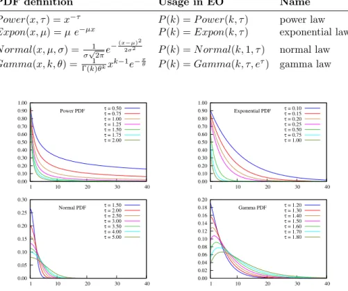
Because it relies on just one parameter, EO is comparatively very simple to use (tuning many local search parameters can become very laborious). As we show in section 4, the results of EO-QAP are very good on many instances of QAPLIB. However, some harder instances need a fine control of the trade-off between intensification and diversification. EO handles these two strategies with the same tool: the probability distribution P(k) = k−τ. Depending on the returned value, either the current path continues to be improved (with a high probability) or, in the extreme case, completely abandoned (with a low probability). Every variable has a non-zero chance of being selected and EO is not affected by local extrema. The choice of the probability distributionP has thus a great impact, also determined by its parameterτ, which must be selected by the user. Tuning τ for some hard problems (e.g. tai40a) turned out to be difficult. We therefore decided toextendEO so as to accept different probability distribution functions (PDF). The user can thus choose the most appropriate PDF. For simplicity, all proposed PDFs take a single input parameter τ, the other parameters (if any) being either constant or functionally dependent on τ. We now discuss a few interesting PDFs, and how they are influenced by the singleτ parameter:
PDF definition Usage in EO Name
P ower(x, τ) =x−τ P(k) =P ower(k, τ) power law
Expon(x, µ) =µ e−µx P(k) =Expon(k, τ) exponential law
N ormal(x, µ, σ) = 1
σ√2πe
−(x−µ)2
2σ2 P(k) =N ormal(k,1, τ) normal law
Gamma(x, k, θ) = Γ(k1)θkx
k−1e−x
θ P(k) =Gamma(k, τ, eτ) gamma law
0.00 0.10 0.20 0.30 0.40 0.50 0.60 0.70 0.80 0.90 1.00 1 10 20 30 40 Power PDF τ = 0.50 τ = 0.75 τ = 1.00 τ = 1.25 τ = 1.50 τ = 1.75 τ = 2.00 0.00 0.10 0.20 0.30 0.40 0.50 0.60 0.70 0.80 0.90 1.00 1 10 20 30 40 Exponential PDF ττ = 0.10 = 0.15 τ = 0.20 τ = 0.25 τ = 0.50 τ = 0.75 τ = 1.00 0.00 0.05 0.10 0.15 0.20 0.25 0.30 1 10 20 30 40 Normal PDF τ = 1.50 τ = 2.00 τ = 2.50 τ = 3.00 τ = 3.50 τ = 4.00 τ = 5.00 0.00 0.02 0.04 0.06 0.08 0.10 0.12 0.14 0.16 0.18 0.20 1 10 20 30 40 Gamma PDF τ = 1.20 τ = 1.30 τ = 1.40 τ = 1.50 τ = 1.60 τ = 1.70 τ = 1.80
The EO algorithm behaves very differently, depending on the PDF and the chosen value forτ. Figure 2 shows the curves associated with these PDFs for a size n= 40, picking different values forτ. Clearly, with the power law, the first ranked variable has a very high probability to be selected, the probability then decreases very fast but the variables with a high rank (i.e.“good” variables) are very likely to mutate (e.g. when τ = 0.5). This results in less intensification, and suits some problems perfectly. If this behavior is unwanted, a larger value forτ may be used, nevertheless, this rapidly puts too strong a pressure on the besk ranked variables which, for some problems, will be selected too frequently. It can be difficult to find a good trade-off. On the other hand, the exponential law skews probabilities a little bit more in favor of lower ranked variables. This is clear from the shapes of the PDFs (see Figure 2). The normal (Gaussian) law is also interesting because the curve decreases slowly for the very first ranks, then more rapidly and then more slowly again: the first ranked “worst” variables will then be selected with a high but comparable priority. Finally, we found the gamma law interesting because it is not strictly decreasing and can, for instance, give more priority to the second or third variable than to the first one. With this PDF we obtained good results fortai40awithτ = 1.5. It is worth noticing that a shifted normal law can also be used as a non-stricly decreasing function, e.g. using P(k) = N ormal(k,2, eτ). It is worth noticing that the best PDF and τ combination is not the same when EO-QAP is run sequentially or in parallel.
Clearly, allowing different PDFs enhances the power of EO which can attack more problems efficiently. The user now has more precise control over the behav-ior of the algorithm, which remains simple with only two tunable parameters: the PDF and its τ value. It is even possible allow the user to provide his own customized PDF as a file ofnvaluesP1, . . . Pn. At run-time, theprob[] array
above mentionned is populated as follows:prob[k]= Pk
Pn
i=1Pi (each value being
divided by the sum of all values to ensure the whole PDF = 1).
4
Experimental Evaluation
In this section we present experimental results on the entire QAPLIB test set. To do this, we developed an X10 implementation of EO-QAP.3 Because EO is a stochastic procedure, we ran each problem 10 times and averaged the results. The number of possible experiments is very high: with different PDFs andτ values, varying the timeout, testing sequential or parallel runs, with different topologies and communication strategies, etc. We thus adopted a 3-stage protocol:
1. Attempt to solve all QAPLIB problems (134 instances) with a basic version of EO-QAP (i.e. without any tuning) and a very short timeout (in order to be able to try 10 runs for each of the 134 instances). All problems for which the Best Known Solution (BKS) was reached for every execution are definitively classified assolved. The others (solved less than 10 times) form the test set of the next stage.
3
2. To attack the remaining problem we ran EO-QAP (with same parameters and timeout) in independent parallel multi-walks, without communication, on 32 cores of a single machine. As previously, we collected the fully solved instances which need no longer be considered. The remaining instances form the input set for the next stage.
3. The remaining problems are the hardest ones: for these, we used a coopera-tive parallel version of EO-QAP on 128 cores, tuning the PDF andτ value, and using a larger timeout of 10 minutes.
4.1 Stage 1: Sequential Execution
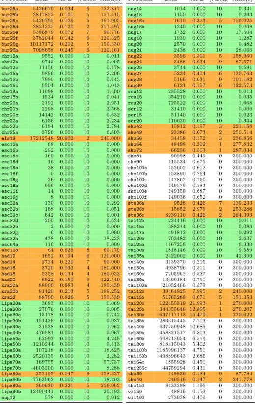
In this first stage, the input test set consists of the 134 QAPLIB instances, which are run sequentially on an AMD Opteron 6376 clocked at 2.3 GHz, using a single core. This is the basic version of EO-QAP with the original power-law PDF and default value forτ(see Section 2.2). For each problem we report the BKS (which is sometimes the optimum), the number of times the BKS is reached (#BKS), i.e. the number of times the problem is solved, the average execution time (in seconds) and the the Average Percentage Deviation (APD) which is the average of the 10 relative deviationpercentages computed as follows: 100F(solBKS)−BKS. We use a short timeout of 5 minutes. Even if the solver stops as soon as the BKS is reached a limited timeout is needed to be able to run the 134 instances 10 times. Table 1 presents the whole results. Surprisingly, even with this straightfor-ward and suboptimal setting, EO-QAP performs quite well: more than 50% of the instances get totally solved. More precisely: 68 instances are fully solved (in green), and among the remaining 66, only 25 are never solved. On average, the 41 others are solved 4.6 times (in orange). The average APD for the 66 instances not fully solved is about 2.2%.
4.2 Stage 2: Independent Parallelism
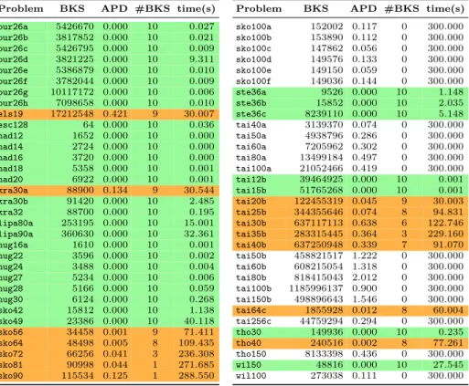
In this stage, we ran the EO-QAP algorithm in parallel without communication with the same settings as in the first stage (default PDF, default τ, timeout 5 min). The machine was the same: a quad AMD Opteron 6376 clocked at 2.3 GHz, but using 32 cores. These parameters make it possible to assess what im-provement we can easily obtain by means of parallel execution. Indeed, this from of parallelism (sometimes called embarrassingly parallelism) works by perform-ing multiple independent walks to explore the search space. Each worker blindly explores a region of the search space, looking for a solution. The process ends as soon as any solver reaches a solution. Since all EO solvers start from a ran-dom point, we can expect that they will all visit different regions of the search space (i.e. ensuring a form of diversification), thus increasing the chance to find a solution. Such a parallelization of an algorithm is easy to implement and often behaves very well (see Section 2.3).
The results of this experiment are summarized in Table 2. This form of parallelism brings a significant improvement in performance and reach. Exactly
Problem BKS APD #BKS time(s) bur26a 5426670 0.034 6 122.817 bur26b 3817852 0.101 5 151.415 bur26c 5426795 0.126 5 161.905 bur26d 3821225 0.120 2 251.497 bur26e 5386879 0.072 7 90.776 bur26f 3782044 0.142 6 120.325 bur26g 10117172 0.202 5 150.330 bur26h 7098658 0.245 6 120.161 chr12a 9552 0.000 10 0.011 chr12b 9742 0.000 10 0.005 chr12c 11156 0.000 10 0.178 chr15a 9896 0.000 10 2.206 chr15b 7990 0.000 10 0.143 chr15c 9504 0.000 10 1.043 chr18a 11098 0.000 10 1.400 chr18b 1534 0.000 10 0.041 chr20a 2192 0.000 10 2.951 chr20b 2298 0.000 10 3.568 chr20c 14142 0.000 10 0.632 chr22a 6156 0.000 10 2.234 chr22b 6194 0.000 10 2.784 chr25a 3796 0.000 10 6.803 els19 17212548 20.902 2 240.000 esc16a 68 0.000 10 0.000 esc16b 292 0.000 10 0.000 esc16c 160 0.000 10 0.000 esc16d 16 0.000 10 0.000 esc16e 28 0.000 10 0.000 esc16f 0 0.000 10 0.000 esc16g 26 0.000 10 0.000 esc16h 996 0.000 10 0.000 esc16i 14 0.000 10 0.000 esc16j 8 0.000 10 0.000 esc32a 130 0.000 10 0.292 esc32b 168 0.000 10 0.051 esc32c 642 0.000 10 0.001 esc32d 200 0.000 10 6.634 esc32e 2 0.000 10 0.000 esc32g 6 0.000 10 0.000 esc32h 438 0.000 10 18.223 esc64a 116 0.000 10 0.009 esc128 64 0.625 8 60.175 had12 1652 0.194 6 120.000 had14 2724 0.220 7 90.000 had16 3720 0.032 4 180.000 had18 5358 0.134 4 180.033 had20 6922 0.150 6 122.549 kra30a 88900 0.983 4 180.439 kra30b 91420 0.213 5 189.252 kra32 88700 0.826 5 150.539 lipa20a 3683 0.000 10 0.069 lipa20b 27076 0.000 10 0.005 lipa30a 13178 0.000 10 0.742 lipa30b 151426 0.000 10 0.037 lipa40a 31538 0.000 10 1.962 lipa40b 476581 0.000 10 0.067 lipa50a 62093 0.000 10 4.245 lipa50b 1210244 0.000 10 0.113 lipa60a 107218 0.000 10 18.825 lipa60b 2520135 0.000 10 2.282 lipa70a 169755 0.000 10 57.737 lipa70b 4603200 0.000 10 8.288 lipa80a 253195 0.047 9 158.337 lipa80b 7763962 0.000 10 18.203 lipa90a 360630 0.221 5 256.062 lipa90b 12490441 0.000 10 20.193 nug12 578 0.000 10 0.012
Problem BKS APD #BKS time(s)
nug14 1014 0.000 10 0.341 nug15 1150 0.000 10 0.293 nug16a 1610 0.373 5 150.025 nug16b 1240 0.000 10 0.008 nug17 1732 0.000 10 17.504 nug18 1930 0.000 10 1.287 nug20 2570 0.000 10 0.482 nug21 2438 0.000 10 28.066 nug22 3596 0.501 5 158.960 nug24 3488 0.034 9 87.571 nug25 3744 0.000 10 0.591 nug27 5234 0.474 6 130.763 nug28 5166 0.031 9 101.182 nug30 6124 0.157 6 122.573 rou12 235528 0.000 10 0.013 rou15 354210 0.000 10 0.035 rou20 725522 0.000 10 1.668 scr12 31410 0.000 10 0.006 scr15 51140 0.000 10 0.023 scr20 110030 0.000 10 0.334 sko42 15812 0.197 3 221.158 sko49 23386 0.073 2 250.514 sko56 34458 0.172 3 236.856 sko64 48498 0.302 1 277.832 sko72 66256 0.503 1 287.034 sko81 90998 0.449 0 300.000 sko90 115534 0.675 0 300.000 sko100a 152002 0.612 0 300.000 sko100b 153890 0.264 0 300.000 sko100c 147862 0.760 0 300.000 sko100d 149576 0.583 0 300.000 sko100e 149150 0.687 0 300.000 sko100f 149036 0.652 0 300.000 ste36a 9526 0.426 7 139.233 ste36b 15852 2.976 2 253.286 ste36c 8239110 0.426 2 264.393 tai12a 224416 0.000 10 0.011 tai15a 388214 0.000 10 0.089 tai17a 491812 0.000 10 0.292 tai20a 703482 0.000 10 2.637 tai25a 1167256 0.000 10 6.330 tai30a 1818146 0.000 10 9.589 tai35a 2422002 0.000 10 42.399 tai40a 3139370 0.215 0 300.000 tai50a 4938796 0.511 0 300.000 tai60a 7205962 0.537 0 300.000 tai80a 13499184 0.750 0 300.000 tai100a 21052466 0.579 0 300.000 tai12b 39464925 7.995 2 240.000 tai15b 51765268 0.071 5 151.353 tai20b 122455319 21.993 1 270.000 tai25b 344355646 12.805 1 270.207 tai30b 637117113 15.479 1 270.022 tai35b 283315445 7.703 0 300.000 tai40b 637250948 10.085 0 300.000 tai50b 458821517 6.803 0 300.000 tai60b 608215054 6.559 0 300.000 tai80b 818415043 5.402 0 300.000 tai100b 1185996137 4.750 0 300.000 tai150b 498896643 2.686 0 300.000 tai64c 1855928 0.450 0 300.000 tai256c 44759294 0.431 0 300.000 tho30 149936 0.184 9 87.784 tho40 240516 0.147 2 241.778 tho150 8133398 1.196 0 300.000 wil50 48816 0.153 0 300.000 wil100 273038 0.409 0 300.000
Problem BKS APD #BKS time(s) bur26a 5426670 0.000 10 0.027 bur26b 3817852 0.000 10 0.021 bur26c 5426795 0.000 10 0.009 bur26d 3821225 0.000 10 9.311 bur26e 5386879 0.000 10 0.010 bur26f 3782044 0.000 10 0.009 bur26g 10117172 0.000 10 0.006 bur26h 7098658 0.000 10 0.010 els19 17212548 0.421 9 30.007 esc128 64 0.000 10 0.036 had12 1652 0.000 10 0.000 had14 2724 0.000 10 0.000 had16 3720 0.000 10 0.000 had18 5358 0.000 10 0.001 had20 6922 0.000 10 0.001 kra30a 88900 0.134 9 30.544 kra30b 91420 0.000 10 2.485 kra32 88700 0.000 10 0.195 lipa80a 253195 0.000 10 15.001 lipa90a 360630 0.000 10 32.361 nug16a 1610 0.000 10 0.001 nug22 3596 0.000 10 0.002 nug24 3488 0.000 10 0.004 nug27 5234 0.000 10 0.006 nug28 5166 0.000 10 0.059 nug30 6124 0.000 10 0.268 sko42 15812 0.000 10 1.138 sko49 23386 0.000 10 40.118 sko56 34458 0.001 9 71.411 sko64 48498 0.005 8 109.435 sko72 66256 0.041 3 236.308 sko81 90998 0.044 1 271.685 sko90 115534 0.125 1 288.550
Problem BKS APD #BKS time(s)
sko100a 152002 0.117 0 300.000 sko100b 153890 0.112 0 300.000 sko100c 147862 0.056 0 300.000 sko100d 149576 0.133 0 300.000 sko100e 149150 0.059 0 300.000 sko100f 149036 0.144 0 300.000 ste36a 9526 0.000 10 1.148 ste36b 15852 0.000 10 2.035 ste36c 8239110 0.000 10 5.148 tai40a 3139370 0.074 0 300.000 tai50a 4938796 0.286 0 300.000 tai60a 7205962 0.302 0 300.000 tai80a 13499184 0.497 0 300.000 tai100a 21052466 0.419 0 300.000 tai12b 39464925 0.000 10 0.001 tai15b 51765268 0.000 10 0.001 tai20b 122455319 0.045 9 30.003 tai25b 344355646 0.074 8 94.831 tai30b 637117113 0.638 6 122.746 tai35b 283315445 0.364 3 229.160 tai40b 637250948 0.339 7 91.070 tai50b 458821517 1.222 0 300.000 tai60b 608215054 1.318 0 300.000 tai80b 818415043 2.012 0 300.000 tai100b 1185996137 0.900 0 300.000 tai150b 498896643 1.546 0 300.000 tai64c 1855928 0.012 8 60.004 tai256c 44759294 0.294 0 300.000 tho30 149936 0.000 10 0.235 tho40 240516 0.002 8 77.261 tho150 8133398 0.436 0 300.000 wil50 48816 0.000 10 27.545 wil100 273038 0.111 0 300.000
Table 2: Independent parallelism on 32 cores (timeout = 300 s)
half of the 66 problem instances now become fully solved (the average time being 3.2s). However, among the 33 remaining ones, 19 remain never solved and, on average, the remaining 14 get solved 6 out of 10 times. Moreover, the average APD over the not fully solved 33 is 0.372%. This contrasts with the previous situation (2.2%), which indicates a significant improvement in the quality of solutions: even when the optimum is not reached, the solution which was found is close.
4.3 Stage 3: Cooperative Parallelism
In this final experiment, we attacked the 33 hardest instances with parallelism and cooperation. This was simplified thanks to the CPLS framework which pro-vides the necessary abstraction layers and already handles the communication (see Section 2.3). The sequential EO-QAP needed a very simple adaptation: ev-ery R iterations it has to send its current configuration to the Elite Pool and, every U iterations, it retrieves a configuration from the pool, which it nonde-terministically4adopts it if it is better than the current one. The CPLS system
4
already provides library functions for all these operations. The resulting solver is then composed of several EO-QAP instances running in parallel, which coop-erate by communicating in order to converge faster on a solution. As per [7], the CPLS parameters which control the cooperation are as follows:
– Team Size(N P T): we tested various configurations and definedN P T = 16. There are thus 8 teams composed of 16 explorer nodes each running the EO-QAP procedure. This is constant for all problems.
– Report Interval(R): we manually tuned it (starting from the average number of iterations collected during the previous stage divided by 10).
– Update Interval(U): we experimented different ratio and retainedU/R= 2.
– Elite Pool (EP): its size is fixed to 4 for all problems.
– pAdopt: is set to 1. An EO-QAP instance receiving a better configuration than its current one always switches to this new one.
This experiment has been carried out on a cluster of 16 machines, each with 4 × 16-core AMD Opteron 6376 CPUs running at 2.3 GHz and 128 GB of RAM. The nodes are interconnected with InfiniBand FDR 4×(i.e. 56 GBPS.) We had access to 4 nodes and used up to 32 cores per node, i.e. 128 cores. We stay with a timeout of 5 minutes. Finally, we tested deeply two PDFs (power and exponential) and their τ value and retained the best combination for each problem instance (we could not yet test the Normal law and the Gamma law, while efficient in sequential seems, not well suited for parallelism or else using a differentτ value).
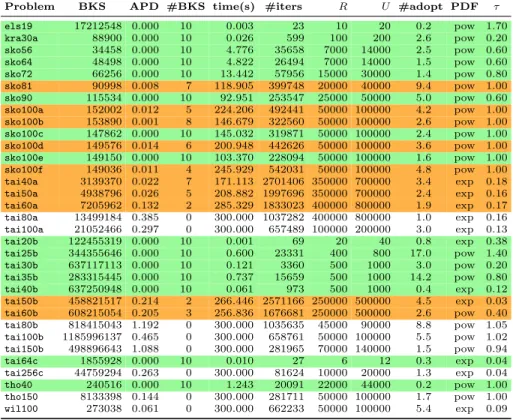
Table 3 presents the results obtained on the hardest instances. The table also reports the average number of iterations, the report and update interval (Rand
U), the number of times the winning algorithm has adopted an elite configu-ration, the PDF and τ value used. In this last stage, 15 new problems become fully solved. Moreover the average time to solve them is only 24.5 seconds. Only 8 remain unsolved. On average, the remaining 10 get solved 5 out of 10 times. Moreover, the average APD over the 18 not fully solved is only 0.25%. Even when the optimum is not reached the returned solution is close to this optimum. The table shows that an efficient execution corresponds to a limited number of “adoptions” of an elite configuration (less than 5 changes). This is directly correlated to the value ofRand U. There are some exceptions like tai25band
tho40 which are both fully solved. We plan to analyze in details these both
situations (e.g. varying R and U).
Regarding the power and exponential PDF, there is no winner. It is worth noticing that sometimes the difference is huge. For instance, sko90 is solved 9 times with the power law but only 2 times with the exponential law. The reverse occurs fortaiXXafor which the exponential law performs much better.
The performance of the cooperative parallel EO-QAP, is on par with the best competing solutions, while retaining a much simpler internal structure [32]. Due to space limitations, we do not develop this further.
Problem BKS APD #BKS time(s) #iters R U #adopt PDF τ els19 17212548 0.000 10 0.003 23 10 20 0.2 pow 1.70 kra30a 88900 0.000 10 0.026 599 100 200 2.6 pow 0.20 sko56 34458 0.000 10 4.776 35658 7000 14000 2.5 pow 0.60 sko64 48498 0.000 10 4.822 26494 7000 14000 1.5 pow 0.60 sko72 66256 0.000 10 13.442 57956 15000 30000 1.4 pow 0.80 sko81 90998 0.008 7 118.905 399748 20000 40000 9.4 pow 1.00 sko90 115534 0.000 10 92.951 253547 25000 50000 5.0 pow 0.60 sko100a 152002 0.012 5 224.206 492441 50000 100000 4.2 pow 1.00 sko100b 153890 0.001 8 146.679 322560 50000 100000 2.6 pow 1.00 sko100c 147862 0.000 10 145.032 319871 50000 100000 2.4 pow 1.00 sko100d 149576 0.014 6 200.948 442626 50000 100000 3.6 pow 1.00 sko100e 149150 0.000 10 103.370 228094 50000 100000 1.6 pow 1.00 sko100f 149036 0.011 4 245.929 542031 50000 100000 4.8 pow 1.00 tai40a 3139370 0.022 7 171.113 2701406 350000 700000 3.4 exp 0.18 tai50a 4938796 0.026 5 208.882 1997696 350000 700000 2.4 exp 0.16 tai60a 7205962 0.132 2 285.329 1833023 400000 800000 1.9 exp 0.17 tai80a 13499184 0.385 0 300.000 1037282 400000 800000 1.0 exp 0.16 tai100a 21052466 0.297 0 300.000 657489 100000 200000 3.0 exp 0.13 tai20b 122455319 0.000 10 0.001 69 20 40 0.8 exp 0.38 tai25b 344355646 0.000 10 0.600 23331 400 800 17.0 pow 1.40 tai30b 637117113 0.000 10 0.121 3360 500 1000 3.0 pow 0.20 tai35b 283315445 0.000 10 0.737 15659 500 1000 14.2 pow 0.80 tai40b 637250948 0.000 10 0.061 973 500 1000 0.4 exp 0.12 tai50b 458821517 0.214 2 266.446 2571166 250000 500000 4.5 exp 0.03 tai60b 608215054 0.205 3 256.836 1676681 250000 500000 2.6 pow 0.40 tai80b 818415043 1.192 0 300.000 1035635 45000 90000 8.8 pow 1.05 tai100b 1185996137 0.465 0 300.000 658761 50000 100000 5.5 pow 1.02 tai150b 498896643 1.088 0 300.000 281965 70000 140000 1.5 pow 0.94 tai64c 1855928 0.000 10 0.010 27 6 12 0.3 exp 0.04 tai256c 44759294 0.263 0 300.000 81624 10000 20000 1.3 exp 0.04 tho40 240516 0.000 10 1.243 20091 22000 44000 0.2 pow 1.00 tho150 8133398 0.144 0 300.000 281711 50000 100000 1.7 pow 1.00 wil100 273038 0.061 0 300.000 662233 50000 100000 5.4 exp 0.09
Table 3: Cooperative parallelism on 128 cores (timeout = 300 s)
5
Conclusion and Further Work
We have proposed EO-QAP: an Extremal Optimization (EO) procedure for QAP. The basic sequential version of EO-QAP, while simple behaves rather well on several instances of QAPLIB. To attack hardest instances we first proposed a simple extension to the original EO procedure allowing for different probabil-ity distribution functions (PDF). The user can select the most adequate PDF depending on the degree of intensification wanted. Moreover, we resorted to co-operative parallelism using a framework written in the X10 parallel language, which provides the user with a fine degree of control of the intensification and diversification for the search. The cooperative version of EO-QAP displays very good results: using 128 cores, 116 instances of QAPLIB are systematically solved at each execution, 10 instances are solved half the time and only 8 instances re-main unsolved (but the obtained solution is near to the optimum).
We now plan to attack other known hard instances. Future work includes the study of a default parameter for the other PDFs (e.g. exponential) and how to take into account the hardness of the problem to define this value (e.g. in terms of the landscape ruggedness of the instance to solve). Moreover, we plan
to explore portfolio approaches, i.e. ones which combine multiple solvers as well as experiment with techniques for parameter auto-tuning. This experimentation entails a deep analysis of the parallel performance behavior.
Acknowledgments
The authors wish to acknowledge Stefan Boettcher (Emory University) for his explanations about the Extremal Optimization method. The experimentation used the cluster of the University of ´Evora, which was partly funded by grants ALENT-07-0262-FEDER-001872 and ALENT-07-0262-FEDER-001876.
References
1. Koopmans, T.C., Beckmann, M.: Assignment Problems and the Location of Eco-nomic Activities. Econometrica25(1) (1957) 53–76
2. Commander, C.W.: A survey of the quadratic assignment problem, with applica-tions. Morehead Electronic Journal of Applicable Mathematics4(2005) MATH– 2005–01
3. Bhati, R.K., Rasool, A.: Quadratic Assignment Problem and its Relevance to the Real World: A Survey. International Journal of Computer Applications96(9) (2014) 42–47
4. Sahni, S., Gonzalez, T.: P-Complete Approximation Problems. Journal of the ACM23(3) (1976) 555–565
5. Boettcher, S., Percus, A.: Nature’s way of optimizing. Artificial Intelligence
119(12) (2000) 275–286
6. Randall, M., Lewis, A.: Intensification Strategies for Extremal Optimisation. In: Simulated Evolution and Learning - 8th International Conference, (SEAL), Kan-pur, India. Volume 6457 of LNCS., Springer (2010) 115–124
7. Munera, D., Diaz, D., Abreu, S., Codognet, P.: A Parametric Framework for Coop-erative Parallel Local Search. In Blum, C., Ochoa, G., eds.: European Conference on Evolutionary Computation in Combinatorial Optimisation (EvoCOP). Volume 8600 of Lecture Notes in Computer Science., Springer (2014) 13–24
8. Charles, P., Grothoff, C., Saraswat, V., Donawa, C., Kielstra, A., Ebcioglu, K., Von Praun, C., Sarkar, V.: X10: An Object-Oriented Approach to Non-Uniform Cluster Computing. In: SIGPLAN Conference on Object-oriented Programming, Systems, Languages, and Applications, San Diego, CA, USA, ACM (2005) 519–538 9. Saraswat, V., Tardieu, O., Grove, D., Cunningham, D., Takeuchi, M., Herta, B.: A Brief Introduction to X10 (for the High Performance Programmer). Technical report (2012)
10. Burkard, R.E.: Quadratic Assignment Problems. In Pardalos, P.M., Du, D.Z., Gra-ham, R.L., eds.: Handbook of Combinatorial Optimization (2nd edition). Springer New York (2013) 2741–2814
11. Loiola, E.M., de Abreu, N.M.M., Netto, P.O.B., Hahn, P., Querido, T.M.: A survey for the quadratic assignment problem. European Journal of Operational Research
176(2) (2007) 657–690
12. Zaied, A.N.H., Shawky, L.A.E.f.: A Survey of Quadratic Assignment Problems. International Journal of Computer Applications101(6) (2014) 28–36
13. Said, G.A.E.N.A., Mahmoud, A.M., El-Horbaty, E.S.M.: A Comparative Study of Meta-heuristic Algorithms for Solving Quadratic Assignment Problem. Inter-national Journal of Advanced Computer Science and Applications (IJACSA)5(1) (2014)
14. Boettcher, S., Percus, A.G.: Extremal Optimization: an Evolutionary Local-Search Algorithm. In: Computational Modeling and Problem Solving in the Networked World. Volume 21. Springer US (2003)
15. Boettcher, S.: Extremal Optimization. In Hartmann, A.K., Rieger, H., eds.: New Optimization Algorithms to Physics. Wiley-VCH Verlag, Berlin (2004) 227–251 16. Bak, P., Tang, C., Wiesenfeld, K.: Self-Organized Crtiticality: An Explenation of
1/f Noise. Physical Review Letters59(4) (1987) 381–384
17. Bak, P.: How Nature Works: The Science of Self-organized Criticality. 1st edn. Copernicus (Springer) (1996)
18. Bak, P., Sneppen, K.: Punctuated equilibrium and criticality in a simple model of evolution. Physical Review Letters71(24) (1993) 4083–4086
19. Boettcher, S., Percus, A.G.: Optimization with Extremal Dynamics. Physical Review Letters86(23) (2001) 5211–5214
20. De Sousa, F.L., Ramos, F.M.: Function optimization using extremal dynamics. International Conference on Inverse Problems in Engineering Rio de Janeiro, Brazil (2002)
21. De Sousa, F.L., Vlassov, V., Ramos, F.M.: Generalized Extremal Optimization for Solving Complex Optimal Design Problems. International Conference on Genetic and Evolutionary Computation (2003) 375–376
22. Zhou, T., Bai, W.J., Cheng, L.J., Wang, B.H.: Continuous Extremal Optimization for Lennard-Jones Clusters. Physical Review E72(1) (2005)
23. Alba, E.: Parallel Metaheuristics: A New Class of Algorithms. Wiley-Interscience (2005)
24. Alba, E., Luque, G., Nesmachnow, S.: Parallel Metaheuristics: Recent Advances and New Trends. International Transactions in Operational Research20(1) (2013) 1–48
25. Diaz, D., Abreu, S., Codognet, P.: Parallel Constraint-Based Local Search on the Cell/BE Multicore Architecture. In: Studies in Computational Intelligence. Volume 315. (2010) 265–274
26. Verhoeven, M., Aarts, E.: Parallel Local Search. Journal of Heuristics1(1) (1995) 43–65
27. Caniou, Y., Codognet, P., Richoux, F., Diaz, D., Abreu, S.: Large-scale parallelism for constraint-based local search: the costas array case study. Constraints20(1) (2014) 1–27
28. Toulouse, M., Crainic, T., Sans´o, B.: Systemic Behavior of Cooperative Search Algorithms. Parallel Computing (2004) 57–79
29. Munera, D., Diaz, D., Abreu, S., Codognet, P.: Flexible Cooperation in Parallel Local Search. In: Symposium on Applied Computing (SAC), New York, New York, USA, ACM Press (2014) 1360–1361
30. Minton, S., Philips, A., Johnston, M.D., Laird, P.: Minimizing Conflicts: A Heuris-tic Repair Method for Constraint-Satisfaction and Scheduling Problems. Journal of Artificial Intelligence Research58(1993) 161–205
31. Taillard, ´E.D.: Comparison of iterative searches for the quadratic assignment prob-lem. Location Science3(2) (1995) 87–105
32. James, T., Rego, C., Glover, F.: A Cooperative Parallel Tabu Search Algorithm for the Quadratic Assignment Problem. European Journal of Operational Research (2009)