A Bayesian Approach to Two-Mode Clustering
∗
Bram van Dijk
Tinbergen Institute
Econometric Institute
Erasmus University Rotterdam
Joost van Rosmalen
Erasmus Research Institute of Management
Econometric Institute
Erasmus University Rotterdam
Richard Paap
Econometric Institute
Erasmus University Rotterdam
ECONOMETRIC INSTITUTE REPORT EI 2009-06
AbstractWe develop a new Bayesian approach to estimate the parameters of a latent-class model for the joint clustering of both modes of two-mode data matrices. Posterior results are obtained using a Gibbs sampler with data augmentation. Our Bayesian approach has three advantages over existing methods. First, we are able to do statistical inference on the model parameters, which would not be possible using frequentist estimation procedures. In addition, the Bayesian approach allows us to provide statistical criteria for determining the optimal numbers of clusters. Finally, our Gibbs sampler has fewer problems with local optima in the likelihood function and empty classes than the EM algorithm used in a frequentist approach. We apply the Bayesian estimation method of the latent-class two-mode clustering model to two empirical data sets. The first data set is the Supreme Court voting data set of Doreian, Batagelj, and Ferligoj (2004). The second data set comprises the roll call votes of the United States House of Representatives in 2007. For both data sets, we show how two-mode clustering can provide useful insights.
Keywords: two-mode data, model-based clustering, latent-class model, MCMC
∗We thank Dennis Fok for helpful comments. Corresponding author: Richard Paap, Econometric
Institute, Erasmus University Rotterdam, P.O. Box 1738, 3000 DR Rotterdam, The Netherlands, e-mail:
1
Introduction
Clustering algorithms divide a single set of objects into segments based on their similar-ities and properties, or on their dissimilarsimilar-ities, see, for example, Hartigan (1975). Such methods typically operate on one mode (dimension) of a data matrix; we refer to these methods as one-mode clustering. Two-mode clustering techniques (Van Mechelen, Bock, & De Boeck, 2004) cluster two sets of objects into segments based on their interactions. In two-mode clustering, both rows and columns of data matrix are clustered simultaneously. Many clustering methods, such as k-means clustering and Ward’s method, lack a method to ascertain the significance of the results and rely on arbitrary methods to determine the number of clusters. To solve these problems, one may consider model-based techniques for clustering data. For one-mode data, model-based clustering methods have been developed, see, for example, Fraley and Raftery (1998); Wedel and Kamakura (2000); Fr¨uhwirth-Schnatter (2006). These model-based clustering methods use statistical tools for inference.
In this article, we extend the model-based one-mode clustering approach to two-mode clustering. In two-mode clustering, we cluster both the rows and the columns of a data matrix into groups in such a way that the resulting block structure is homogenous within blocks but differs between blocks. This requires matrix-conditional data, which means that all elements must be comparable in size, standardized, or measured on the same scale. Methods for two-mode clustering are in general not model-based (see, for example, Candel & Maris, 1997; Doreian et al., 2004; Brusco & Steinley, 2006; Van Rosmalen, Groenen, Trejos, & Castillo, 2009). One-mode model-based clustering methods usually rely on latent-class techniques. It is not straightforward to extend these techniques to two-mode data, because, unlike one-mode data, two-mode data cannot be assumed to be independent. Despite this problem, Govaert and Nadif (2003, 2008) have been able to use a latent-class approach to cluster two-mode data. They use a frequentist approach to estimate the parameters, but they are only able to optimize an approximation of the likelihood function using the EM algorithm (Dempster, Laird, & Rubin, 1977). In this article, we use the same likelihood function as Govaert and Nadif (2003, 2008), but
we propose a Bayesian estimation procedure. This enables us to estimate the model parameters properly and to do statistical inference on the estimation results.
The contribution of our Bayesian approach is threefold. First, our approach allows for statistical inference on the parameter estimates. Govaert and Nadif (2003, 2008) estimate the model parameters in a frequentist setting, but they are unable to compute standard errors of the estimated parameters. Our Bayesian approach provides posterior distributions and hence posterior standard deviations of the parameters. Therefore, our approach enables hypothesis testing, which is not feasible in the frequentist setting.
Secondly, our Bayesian method has fewer computational problems than the maximum likelihood approach. Using proper priors, we avoid some computational issues with empty classes, which is a well known problem when using the EM algorithm for finite mixture models. Posterior results can be obtained using Gibbs sampling with data augmentation (Tanner & Wong, 1987). Because of the more flexible way Markov Chain Monte Carlo methods search the parameter space, our Bayesian approach is less likely to get stuck in a local optimum of the likelihood function. This flexibility may cause label switching, see Celeux, Hurn, and Robert (2000). However, solutions to this problem exist (see, for example, Fr¨uhwirth-Schnatter, 2001; Geweke, 2007).
Finally, our method can help indicate the optimal number of segments. The Bayesian approach can be used to derive selection criteria such as Bayes factors. Methods pre-viously proposed in the literature for selecting the optimal number of clusters (see, for example, Milligan & Cooper, 1985; Schepers, Ceulemans, & Mechelen, 2008) seem some-what arbitrary and lack theoretical underpinnings.
We illustrate our Bayesian approach using two data sets. The first data set comprises votes of the Supreme Court of the United States and was also used by Doreian et al. (2004). Our approach results in a similar solution; however, the optimal numbers of segments are lower than in their solution. Our second application is a large data set concerning roll call voting in the United States House of Representatives. We use our model to cluster both the representatives and the bills simultaneously.
The remainder of this paper is organized as follows. In Section 2 we introduce our new Bayesian approach for clustering two-mode data. We compare this Bayesian approach
with the existing frequentist approaches of Govaert and Nadif (2003, 2008). In Section 3, we discuss the posterior simulator for our Bayesian approach and the selection of the numbers of segments. In Section 4, the Bayesian approach is illustrated on the Supreme Court voting data. Section 5 deals with our second application, which concerns roll call votes of the United States House of Representatives in 2007. Finally, Section 6 concludes.
2
The Latent-Class Two-Mode Clustering Model
In this section, we present our Bayesian approach to clustering both modes of two-mode data simultaneously. We first give a derivation of the likelihood function and then discuss Bayesian parameter estimation for the latent-class two-mode clustering model.
2.1
The Likelihood Function
For illustrative purposes, we start this discussion with one-mode data, that is, we have
N observations denoted by y = (y1, . . . , yN)0. These observations can be discrete or
continuous, and one-dimensional or multidimensional. We assume that each observation comes from one of K segments, and that the elements within each segment are indepen-dently and identically distributed. As a result, all observations must be independent. Furthermore, we assume that the observations come from a known distribution which is the same across segments; only the parameters of the distribution vary among the seg-ments. These data can be described by a mixture model. Let ki ∈ {1, . . . , K} be an
indicator for the segment to which observation yi belongs, and let k= (k1, . . . , kN)0. The
conditional density ofyi belonging to segment qonly depends on the parameter vectorθq
and is denoted by g(yi|θq). The segment membership is unknown. We assume that the
probability that observation yi belongs to segmentq is given by κq forq = 1, . . . , K, with
κq > 0 and
PK
q=1κq = 1. We collect the so-called mixing proportions κq in the vector
κ= (κ1, . . . , κK)0. The likelihood function of this model is given by
l(y|θ, κ) = N Y i=1 ( K X q=1 κqg(yi|θq) ) , (1) where θ= (θ1, . . . , θK)0.
To cluster two-mode data, we would like to extend (1) to two-mode data matrices, with a simultaneous clustering of both rows and columns. We aim to construct a model in which the observations that belong to the same row cluster and the same column cluster are independently and identically distributed. In two-mode clustering, unlike in one-mode clustering, this assumption does not ensure that all observations are independent. As a result, a naive extension of the one-mode likelihood function to two modes will not adequately describe the dependence structure in the data.
Assume that Y is an (N×M) matrix with elementsYi,j, and that we want to cluster
the rows intoK latent classes and the columns intoLlatent classes. The naive extension of (1) to two-mode data yields
lnaive(Y|θ, κ, λ) = N Y i=1 M Y j=1 K X q=1 L X r=1 κqλrg(Yi,j|θq,r), (2)
where κ = (κ1, . . . , κK)0 gives the size of each row segment, λ = (λ1, . . . , λL)0 gives the
size of each column segment, and θq,r contains the parameters of observations belonging
to row segment q and column segment r. Model (2) fails to impose that all elements in a row belong to the same row cluster and also does not impose that all elements in a column belong to the same column cluster; using this model, the data matrix Y would effectively be modeled as a vector of one-mode data.
To derive the proper likelihood function, we first rewrite the one-mode likelihood function (1) as l(y|θ, κ) = N Y i ( K X q=1 κqg(yi|θq) ) = ( K X q=1 κqg(y1|θq) ) ( K X q=1 κqg(y2|θq) ) . . . ( K X q=1 κqg(yN|θq) ) = K X k1=1 K X k2=1 · · · K X kN=1 N Y i=1 κkig(yi|θki) = X k∈K K Y q=1 κNkq q N Y i=1 g(yi|θki), (3)
where we introduce some new notation in the last line. First, the setKcontains all possible divisions of the observations into the segments and thus has KN elements if there are N
observations and K possible segments. Second, Nkq equals the number of observations belonging to segment q according to segmentation k. Thus, PKq=1Nkq = N for a fixed classification k. The fact that these two representations of the likelihood function of a mixture model are equivalent was already noticed by Symons (1981).
Using this representation, we can extend the mixture model to clustering two modes simultaneously. The resulting likelihood function for two modes is
l(Y|θ, κ, λ) = X k∈K X l∈L K Y q=1 κNkq q L Y r=1 λMlr r N Y i=1 M Y j=1 g(Yi,j|θki,lj), (4)
whereLdenotes all possible divisions of the columns intoLsegments,Mr
l equals the
num-ber of items belonging to segment r according to column segmentation l = (l1, . . . , lM)0.
Note that it is impossible to rewrite (4) as a product of likelihood contributions as is possible in the one-mode case (1).
2.2
Parameter Estimation
The likelihood function (4) was already proposed by Govaert and Nadif (2003), who estimate the parameters of this model in a frequentist setting. However, their approach has several limitations. First, in contrast to the likelihood function in the one-mode case, the likelihood function (4) cannot be written as a product over marginal/conditional likelihood contributions; we only have a sample of size 1 from the joint distribution of Y,
k, andl. Therefore, the standard results for the asymptotic properties of the maximum likelihood estimator are not applicable.
Second, standard approaches to maximize the likelihood function (4) and estimate the model parameters are almost always computationally infeasible. Enumerating the
KNLM possible ways to assign the rows and columns to clusters in every iteration of an
optimization routine is only possible for extremely small data sets. To solve this problem, Govaert and Nadif (2003) instead consider the so-classed classification likelihood approach, in which kand l are parameters that need to be optimized. Hence one maximizes
l(Y;k,l|θ, κ, λ) = K Y q=1 κNkq q L Y r=1 λMlr r N Y i=1 M Y j=1 g(Yi,j|θki,lj) (5)
with respect to θ, κ, λ, k ∈ K, and l ∈ L. As the parameter space contains discrete parameters k and l, standard asymptotic theory for maximum likelihood parameter es-timation does not apply. Govaert and Nadif (2008) also consider the optimization of an approximation to the likelihood function (4). This approximation is based on the assump-tion that the two classificaassump-tions (that is, the classificaassump-tion of the rows and the classificaassump-tion of the columns) are independent.
We solve the aforementioned problems by considering a Bayesian approach. This approach has several advantages. First, we do not have to rely on asymptotic theory for inference. We can use the posterior distribution to do inference on the model parameters. In addition, it turns out that we do not need to evaluate the likelihood specification (4) to obtain posterior results. Posterior results can easily be obtained using a Markov Chain Monte Carlo [MCMC] sampler (Tierney, 1994) with data augmentation (Tanner & Wong, 1987). Data augmentation implies that the latent variables k and lare simulated alongside the model parametersθ,κ, andλ. This amounts to applying the Gibbs sampler to the complete data likelihood in (5). As Tanner and Wong (1987) show, the posterior results for the complete data likelihood function are equal to the posterior results for the likelihood function. As we can rely on the complete data likelihood (5) and do not have to consider (4), obtaining posterior results is computationally feasible. Furthermore, unlike previous studies (see, for example, Govaert & Nadif, 2003, 2008), we can provide statistical rules for choosing the numbers of segments as will be shown in Section 3.2. Finally, our method does not suffer much from computational difficulties when searching the global optimum of the likelihood function. The EM algorithm is known to get stuck in local optima of the likelihood function, which often occurs in local optima with one or more empty segments. Because we rely on MCMC methods, our approach has fewer problems with local optima. Furthermore, by using proper priors, we can avoid solutions with empty segments, see also Dias and Wedel (2004) for similar arguments.
3
Posterior Simulator
As discussed previously, we rely on MCMC methods to estimate the posterior distributions of the parameters of the two-mode mixture model. We propose a Gibbs sampler (Geman & Geman, 1984) with data augmentation (Tanner & Wong, 1987), in which we sample the vectors k and l alongside the model parameters. This approach allows us to sample from the posterior distributions of the parameters without evaluating the full likelihood function and therefore requires limited computation time. We assume independent priors for the model parameters with density functions f(κ), f(λ), and f(θ). In Section 3.1, we derive the Gibbs sampler. Methods for choosing the numbers of segments are discussed in Section 3.2.
3.1
The Gibbs Sampler
In each iteration of the Gibbs sampler, we sample the parameters θ, κ, and λ together with the latent variables k and l from their full conditional distributions. The MCMC simulation scheme is as follows:
• Draw κ, λ|θ,k,l,Y
• Draw k|κ, λ, θ,l,Y
• Draw l|κ, λ, θ,k,Y
• Draw θ|κ, λ,k,l,Y
Below we derive the full conditional posteriors, which are needed for the Gibbs sampler. After convergence of the sampler, we obtain a series of draws from the posterior distribu-tions of the model parameters θ,κ, and λ. These draws can be used to compute posterior means, posterior standard deviations, and highest posterior density regions. Because we use data augmentation, we also obtain draws from the posterior distributions of k and
l. This enables us to compute the posterior distributions of each row of data and each column of data over the segments. We can store the posterior distributions in matricesQ
posterior distribution of a row of data over the K possible row segments, and each row of R contains the posterior distribution of a column of data over the L possible column segments.
Sampling of κ and λ
The full conditional density of κ is given by
f(κ|θ, λ,k,l,Y) ∝ l(Y;k,l|θ, κ, λ)f(κ) ∝ K Y q=1 κPNi=1I(ki=q) q f(κ), (6)
wherel(Y;k,l|θ, κ, λ) is the complete data likelihood function given in (5), where f(κ) is the prior density ofκ, and whereI(.) is an indicator function that equals 1 if the argument is true and 0 otherwise. The first part of (6) is the kernel of a Dirichlet distribution, see, for example, Fr¨uhwirth-Schnatter (2006). If we specify a Dirichlet(d1, d2, . . . , dK)
prior distribution for κ, the full conditional posterior is also a Dirichlet distribution with parameters PNi=1I(ki = 1) +d1,
PN
i=1I(ki = 2) +d2,. . .,
PN
i=1I(ki =K) +dK.
If we take a Dirichlet(d1, d2, . . . , dL) prior for λ, the λ parameters can be sampled in
exactly the same way. The full conditional posterior density is now given by
f(λ|θ, κ,k,l,Y)∝ L Y r=1 λ PM j=1I(lj=r) r f(λ), (7)
wheref(λ) denotes the prior density. Hence, we can sampleλfrom a Dirichlet distribution with parameters PMj=1I(lj = 1) +d1, PM j=1I(lj = 2) +d2, . . . , PM j=1I(lj =L) +dL. Sampling of k and l
We sample each element of k and lseparately. The full conditional density of ki is given
by p(ki|θ, κ, λ,k−i,l,Y)∝κki M Y j=1 g(Yi,j|θki,lj) (8)
for ki = 1, . . . , K, where k−i denotes k without ki, and Yi denotes the ith row of Y.
derive the full conditional density of lj, which equals p(lj|θ, κ, λ,k,l−j,Y)∝λlj N Y i=1 g(Yi,j|θki,lj), (9)
where l−j denotesl without lj. We can thus sample lj from a multinomial distribution.
Sampling of θ
The sampling of the parameters θ depends on the specification of g(Yi,j|θq,r). With our
application in mind and for illustrative purposes, we discuss below the sampling of the model parameters for the case where Yi,j follows a Bernoulli or a Normal distribution.
Example 1: Bernoulli Distribution
IfYi,j is a binary random variable with a Bernoulli distribution, with probabilitypq,r when
belonging to row segment q and column segmentr, the density is given by
g(Yi,j|θq,r) =Yi,jpq,r(1−Yi,j)1−pq,r. (10)
Let P denote the (K×L) matrix containing these probabilities for each combination of a row segment and a column segment, so that θ=P.
To sample pq,r, we need to derive its full conditional density, which is given by
f(pq,r|P−q,r, κ, λ,k,l,Y) ∝ Y i∈Q Y j∈R pYi,j q,r (1−pq,r)1−Yi,jf(pq,r) ∝ p PN i=1 PM j=1I(ki=q)I(lj=r)Yi,j q,r (1−pq,r) PN i=1 PM j=1I(ki=q)I(lj=r)(1−Yi,j)f(p q,r), (11)
where Q is the set containing all rows that belong to segment q, where R contains all columns that belong to segment r, where P−q,r denotesPwithout pq,r, and wheref(pq,r)
denotes the prior density ofpq,r. The first part of (11) is the kernel of a Beta distribution.
If we specify a Beta(b1, b2) prior distribution, the full conditional posterior distribution
is also a Beta distribution with parameters PNi=1PMj=1I(ki = q)I(lj = r)Yi,j +b1 and
PN
i=1
PM
Example 2: Normal Distribution
If Yi,j is a normally distributed variable,with mean µq,r and variance σ2q,r in row segment
q and column segment r, we have
g(Yi,j|θq,r) = 1 p 2πσ2 q,r exp ½ −1 2 (Yi,j−µq,r)2 σ2 q,r ¾ . (12)
Letµµµ and Σ denote the (K×L) matrices containing the means and variances for each combination of a row segment and a column segment, respectively; hence θ={µµµ,Σ}.
To sample µq,r, we need to derive its full conditional distribution, which density is
given by f(µq,r|µµµ−q,r,Σ, κ, λ,k,l,Y) ∝ exp " − P i∈Q P j∈R(Yi,j −µq,r)2 2σ2 q,r # f(µq,r) ∝ exp " −(µq,r−1/N q,r k,l P i∈Q P j∈RYi,j)2 2σ2 q,r/Nkq,r,l # f(µq,r), (13)
whereµµµ−q,r denotesµµµwithoutµq,r, and wheref(µq,r) denotes the prior density ofµq,r. The
number of observations that are both in row segment q and column segment r according to segmentations k and l is denoted by Nkq,r,l = PNi=1PMj=1I(ki = q)I(lj = r). As some
segments may become empty in one of the iterations of the Gibbs sampler, we propose to use a proper prior specification for the elements ofµµµandΣ. To facilitate sampling we opt for conjugate priors and specify independent normal prior distributions for the elements ofµµµwith meanµ0 and variance σ20. This results in the following full conditional posterior
distribution µq,r|µµµ−q,r,Σ, κ, λ,k,l,Y∼ N µ σ−2 0 σ−2 0 +s−2 µ0+ s−2 σ−2 0 +s−2 ¯ µ,(σ−2 0 +s−2)−1 ¶ , (14) where ¯µ=Pi∈QPj∈RYi,j/Nkq,r,l, the sample average within the cluster ands2 =σ2q,r/Nkq,r,l.
The full conditional density of σ2
q,r is given by f(σq,r2 |µµµ,Σ−q,r, κ, λ,k,l,Y)∝(σq,r2 )N q,r k,l/2exp " − P i∈Q P j∈R(Yi,j −µq,r)2 2σ2 q,r # f(σq,r2 ), (15) where Σ−q,r denotes Σ without σq,r2 , and where f(σq,r2 ) denotes the prior density of σq,r2 .
sampling we specify independent inverted Gamma-2 priors with parameters g1 andg2 for
the elements inΣ. The full conditional posterior of σ2
q,r is therefore an inverted Gamma-2
distribution with parameters Nkq,r,l +g1 and
P
i∈Q
P
j∈R(Yi,j−µq,r)2+g2.
3.2
Selecting the Numbers of Segments
The standard way to determine the numbers of clusters in a finite mixture model in a frequentist framework is to use information criteria such as AIC, AIC-3, BIC, and CAIC (see, for example, Fraley & Raftery, 1998; Andrews & Currim, 2003). The reason for this is that standard tests for determining the optimal number of classes in latent-class models are not valid due to the Davies (1977) problem. Within a Bayesian framework, we can avoid this problem by computing Bayes factors (see, for example, Berger, 1985; Kass & Raftery, 1995; Han & Carlin, 2001). Unlike the hypotheses testing approach, Bayes factors can be used to compare several possibly nonnested models simultaneously; Bayes factors naturally penalize complex models. The Bayes factor for comparing Model 1 with Model 2 is defined as
B21=
f(Y|M2)
f(Y|M1)
, (16)
where f(Y|Mi) denotes the marginal likelihood of model Mi. The marginal likelihood is
defined as the expected value of the likelihood function with respect to the prior, see, for example, Gelman, Carlin, Stern, and Rubin (2003).
Computing the value of the marginal likelihood is not an easy task. Theoretically, its value can be estimated by averaging the likelihood function over draws from the prior distribution. If the support of the prior distribution does not completely match with the support of the likelihood function, the resulting estimate will be very poor. Another strategy is to use the harmonic mean estimator of Newton and Raftery (1994). However, this estimator can be quite unstable. In this article, we estimate the marginal likelihood using the fourth estimator proposed by Newton and Raftery (1994, p. 22), which is also used by DeSarbo, Fong, Liechty, and Saxton (2004) in a similar model. This estimator uses importance sampling to compute the marginal likelihood value. The importance sampling function is a mixture of the prior and the posterior distribution with mixing proportion δ. Using the fact that the marginal likelihood is the expected value of the
likelihood function with respect to the prior, it can be shown that the marginal likelihood
f(Y) can be estimated using the iterative formula
d
f(Y) = δm/(1−δ) +
Pm
i=1(f(Y|ϑ(i))/(δfd(Y) + (1−δ)f(Y|ϑ(i))))
δm/(1−δ)fd(Y) +Pmi=1(δfd(Y) + (1−δ)f(Y|ϑ(i)))−1 , (17)
wheref(Y|ϑ) denotes the likelihood function andmdenotes the number of drawsϑ(i)from
the posterior distribution; for notational convenience, we drop the model indicatorMi. To
apply this formula, we need to choose the valueδ; Newton and Raftery (1994) recommend using a low value of δ, which we set to 0.001 in our application below. Another approach to compute marginal likelihoods is to use the bridge sampling technique of Fr¨uhwirth-Schnatter (2004).
Obtaining an accurate value of the marginal likelihood for any moderately sophisti-cated model tends to be hard, as was noted by Han and Carlin (2001). Therefore, we also propose a simpler alternative method to choose the numbers of segments, based on information criteria. Simulations in Andrews and Currim (2003) suggest that the AIC-3 of Bozdogan (1994) performs well as a criterion for selecting numbers of segments. To evaluate the AIC-3, we need the maximum likelihood value and the number of parameters. To compute the maximum likelihood value, we take the highest value of the likelihood function (5) across the sampled parameters.
Determining the appropriate number of parameters in our two-mode clustering model is not straightforward. The parameters θ, κ, and λ contain wKL, K −1, and L− 1 parameters, respectively, wherewdenotes the number of parameters inθ per combination of a row segment and a column segment. Although k and l contain the same numbers of parameters for all numbers of latent classes, the number of possible values for each parameter increases. We can think of k as representing an (N ×K) indicator matrix, where each row indicates to which segment an object belongs. This means that k and l
representN(K−1) andM(L−1) free parameters, respectively. Hence, the effective total number of parameters is wKL+NK+ML+K +L−M −N −2.
4
Application 1: Supreme Court Voting Data
We apply the latent-class two-mode clustering model to two empirical data sets. The first data set, which is discussed in this section, is the Supreme Court voting data of Doreian et al. (2004). We use this data set to compare the results of our approach with the results of previous authors, and we discuss this data set relatively briefly. The second data set will be analyzed in greater detail in the next section. The Supreme Court voting data set comprises the decisions of the nine Justices of the United States Supreme Court on 26 important issues. The data are displayed in Table 1. In this table, a 1 reflects that the Justice voted with the majority, and a 0 means that the Justice voted with the minority. To describe the votes, we use a Bernoulli distribution with a Beta(1,1) prior for the probability, which is equivalent to a uniform prior on (0,1). Furthermore, we use an uninformative Dirichlet(1,1, . . . ,1) prior for bothκ and λ.
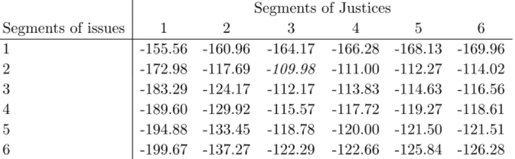
To determine the optimal numbers of segments, we compute the marginal likelihoods for several values of K and L, based on an MCMC chain of 100,000 draws for each combination of K and L. Table 2 displays the values of log marginal likelihoods lnf(Y) for every combination ofK = 1, . . . ,6 rows segments andL= 1, . . . ,6 column segments. The highest marginal likelihood is achieved withK = 2 segments for the issues andL= 3 segments for the Justices. Note that we find fewer segments than Doreian et al. (2004), who applied blockmodeling to this data set and found 7 clusters for the issues and 4 clusters for the Justices, and Brusco and Steinley (2006), who found 5 clusters for the issues and 3 clusters for the Justices.
We experience label switching in our MCMC sampler. Two of the segments of Justices switched places twice in the MCMC chain of 100,000 draws. However, we could easily identify where these switchings occurred. As suggested by Geweke (2007), we solved the label switching problem by sorting the draws in an appropriate way.
To analyze the posterior results, it is possible to weight the results with different numbers of segments according to the posterior model probabilities that follow from the marginal likelihoods. However, we find it more convenient to consider the results for only one value of K and L. Therefore, we focus on the solution with the highest marginal
T able 1: The Supreme Court V oting Data Supreme Court Justice Supreme Court Justice Issue Br Gi So St OC Ke Re Sc Th Issue Br Gi So St OC Ke Re Sc Th 2000 Presiden tial Election 0 0 0 0 1 1 1 1 1 Title VI Disabilities 0 0 0 0 1 1 1 1 1 Illegal Searc h 1 1 1 1 1 1 1 0 0 0 PGA vs. Handicapp ed 1 1 1 1 1 1 1 0 0 Illegal Searc h 2 1 1 1 1 1 1 0 0 0 Immigration Jurisdiction 1 1 1 1 0 1 0 0 0 Illegal Searc h 3 1 1 1 0 0 0 0 1 1 Dep orting Criminal Aliens 1 1 1 1 1 0 0 0 0 Seat Belts 0 0 1 0 0 1 1 1 1 Detaining Criminal Aliens 1 1 1 1 0 1 0 0 0 Sta y of Execution 1 1 1 1 1 1 0 0 0 Citizenship 0 0 0 1 0 1 1 1 1 F ederalism 0 0 0 0 1 1 1 1 1 Legal Aid for the P o or 1 1 1 1 0 1 0 0 0 Clean Air Act 1 1 1 1 1 1 1 1 1 Priv acy 1 1 1 1 1 1 0 0 0 Clean W ater 0 0 0 0 1 1 1 1 1 F ree Sp eec h 1 0 0 0 1 1 1 1 1 Cannabis for Health 0 1 1 1 1 1 1 1 1 Campaign Finance 1 1 1 1 1 0 0 0 0 United F o o ds 0 0 1 1 0 1 1 1 1 T obacco Ads 0 0 0 0 1 1 1 1 1 New Y ork Times Cop yrigh t 0 1 1 0 1 1 1 1 1 Lab or Righ ts 0 0 0 0 1 1 1 1 1 V oting Righ ts 1 1 1 1 1 0 0 0 0 Prop ert y Righ ts 0 0 0 0 1 1 1 1 1
Table 2: Log marginal likelihoods for the Supreme Court Voting Data Segments of Justices Segments of issues 1 2 3 4 5 6 1 -155.56 -160.96 -164.17 -166.28 -168.13 -169.96 2 -172.98 -117.69 -109.98 -111.00 -112.27 -114.02 3 -183.29 -124.17 -112.17 -113.83 -114.63 -116.56 4 -189.60 -129.92 -115.57 -117.72 -119.27 -118.61 5 -194.88 -133.45 -118.78 -120.00 -121.50 -121.51 6 -199.67 -137.27 -122.29 -122.66 -125.84 -126.28
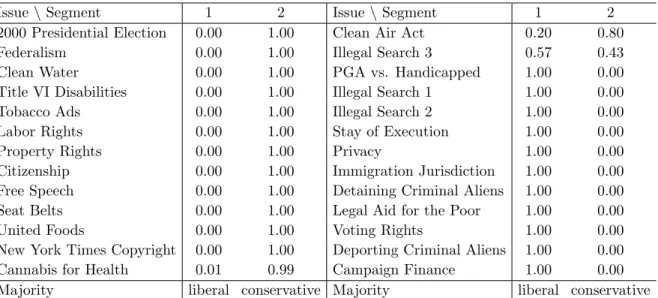
likelihood value, that is, K = 2 segments of issues and L= 3 segments of Justices. The posterior means and standard deviations of P, κ, and λ are shown in Table 3. Tables 4 and 5 show the marginal posterior distributions of the issues and the Justices over the segments. We find that Justices Ginsburg, Stevens, Breyer, and Souter constitute the liberal wing (that is, the left wing) of the Supreme Court. The Court’s moderate wing comprises Justices O’Connor and Kennedy, and the conservative wing (that is, the right wing) consists of Justices Rehnquist, Scalia, and Thomas. The segments of the issues consist of issues that resulted in liberal decisions (segment 1) and issues that resulted in conservative decisions (segment 2). We find strong partisan tendencies in the Supreme Court: liberal Justices support liberal decisions in 97% of the cases, and conservative Justices also support conservative decisions with a 97% probability. The liberal Justices sometimes (in 26% of the cases) vote for a conservative decision, whereas conservative Justices seldom support a liberal decision. Because of their central position in the court, the moderate Justices usually are in the majority. However, the moderate Justices are slightly more likely to support conservative decisions than liberal decisions. In general, the uncertainty in these classifications is low, especially given the relatively small size of the data set. The Justices and almost all issues can be assigned to one segment with a posterior probability close to 1.
The segmentation of the Justices, as displayed in Table 4, resembles the one found by Doreian et al. (2004), who divide the Justices into four segments. The segmentation of the issues deviates more from the solution of Doreian et al. (2004), who find 7 segments for the issues. Brusco and Steinley (2006) also find more segments for the issues than the
Table 3: Posterior means with posterior standard deviations in parentheses, for K = 2 and L= 3 in the Supreme Court Data.
Segment of Justices
Segment of issues 1 2 3 Posterior segment size Interpretation liberal moderate conservative
1 (liberal majority) 0.97 (0.03) 0.68 (0.10) 0.10 (0.07) 0.46 (0.10) 2 (conservative majority) 0.26 (0.07) 0.84 (0.07) 0.97 (0.03) 0.54 (0.10) Posterior segment size 0.42 (0.14) 0.25 (0.12) 0.33 (0.13)
Table 4: Marginal posterior distribution of the Justices over the segments.
Justice 1 2 3 Breyer 1.00 0.00 0.00 Ginsburg 1.00 0.00 0.00 Stevens 1.00 0.00 0.00 Souter 1.00 0.00 0.00 O’Connor 0.00 1.00 0.00 Kennedy 0.00 0.98 0.02 Rehnquist 0.00 0.00 1.00 Thomas 0.00 0.00 1.00 Scalia 0.00 0.00 1.00 Interpretation liberal moderate conservative
Table 5: Marginal posterior distribution of the issues over the segments.
Issue\ Segment 1 2 Issue\ Segment 1 2
2000 Presidential Election 0.00 1.00 Clean Air Act 0.20 0.80 Federalism 0.00 1.00 Illegal Search 3 0.57 0.43 Clean Water 0.00 1.00 PGA vs. Handicapped 1.00 0.00 Title VI Disabilities 0.00 1.00 Illegal Search 1 1.00 0.00 Tobacco Ads 0.00 1.00 Illegal Search 2 1.00 0.00 Labor Rights 0.00 1.00 Stay of Execution 1.00 0.00 Property Rights 0.00 1.00 Privacy 1.00 0.00 Citizenship 0.00 1.00 Immigration Jurisdiction 1.00 0.00 Free Speech 0.00 1.00 Detaining Criminal Aliens 1.00 0.00 Seat Belts 0.00 1.00 Legal Aid for the Poor 1.00 0.00 United Foods 0.00 1.00 Voting Rights 1.00 0.00 New York Times Copyright 0.00 1.00 Deporting Criminal Aliens 1.00 0.00 Cannabis for Health 0.01 0.99 Campaign Finance 1.00 0.00 Majority liberal conservative Majority liberal conservative
numbers of segments found here. We believe that the methods used by these authors may overestimate the numbers of segments in the data.
5
Application 2: Roll Call Voting Data
5.1
Data
To apply our method to a larger data set, we consider the voting behavior of the entire United States House of Representatives. The details of each roll call vote of the United States congress are published on the website http://www.GovTrack.us. We gathered data on all roll call votes from the House of Representatives in 2007. We only use data on votes that are related to a bill. We thus obtain data on 766 roll call votes from 427 members of the House of Representatives in 2007. There are four possible types of votes:
yea, nay, no vote, and present. A no vote means that the representative was absent at the moment of voting; this is the case for 3.5% of the observations. Apresent vote means that the representative is present, but votes neither yea nor nay, which happens only 143 times (0.00%). In contrast to the previous example, we now do not recode our data in such a way that the majority vote is 1 or that the majority vote of the Democrats is 1 to avoid any form of preclustering.
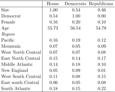
We collected some additional information on the representatives from GovTrack.us. We have data on their party membership, gender, age on January 1st 2007, and state from which they were elected. Table 6 shows the means for these variables for the entire House of Representatives and for the Democrats and Republicans separately. In 2007, the Democrats had a majority in the House of 53.9%, and there were no third-party or independent representatives. There is a fairly large difference in the share of female repre-sentatives between the Democrats (20.4%) and the Republicans (10.1%). The average age is about the same for representatives from both parties. We divided the representatives’ home states into nine regions.
We also collected more information on the bills. Before a bill comes to a vote in the House of Representatives, it is prepared by at least one of the 20 House Committees. Table 7 shows the committees and how many bills they prepared. The committee that
Table 6: Sample means of the individual char-acteristics for the whole House, Democrats, and Republicans.
House Democrats Republicans
Size 1.00 0.54 0.46 Democrat 0.54 1.00 0.00 Female 0.16 0.20 0.10 Age 55.73 56.54 54.78 Region Pacific 0.16 0.19 0.12 Mountain 0.07 0.05 0.09 West North Central 0.07 0.07 0.08 East North Central 0.15 0.14 0.17 Middle Atlantic 0.14 0.18 0.10 New England 0.05 0.09 0.01 West South Central 0.11 0.08 0.15 East south Central 0.06 0.05 0.08 South Atlantic 0.18 0.15 0.22
handles the largest number of bills is Appropriations, which controls the disbursement of funds. The Rules committee influences what is discussed and voted upon; this com-mittee is not primarily concerned with bills and only prepared nine of them. Most other committees deal with specific topics. The committee(s) that prepared a bill provides an indication for the subject of the bill. Having this information should allow us to inter-pret the segments of bills. Identifying the segments of bills may help us understand the segments of representatives in a better way, as we know what types of bills they support and oppose.
Roll call votes have been analyzed before. Poole and Rosenthal (1991), Heckman and Table 7: The numbers of bills prepared by each House Committee
Administration 14 Intelligence (Permanent Select) 15
Agriculture 18 Judiciary 51
Appropriations 291 Natural Resources 50 Armed Services 43 Oversight and Government Reform 57
Budget 14 Rules 9
Education and Labor 51 Science and Technology 43 Energy and Commerce 44 Small Business 26 Financial Services 98 Transportation and Infrastructure 69 Foreign Affairs 44 Veterans’ Affairs 15 Homeland Security 55 Ways and Means 42
Snyder Jr. (1997), and Nelson (2002) try to estimate latent preferences of representa-tives, based on their voting behavior. De Leeuw (2006) plots the relative positions of representatives into a two-dimensional space. The paper that most closely resembles our analysis is Hartigan (2000), who clusters the members of the United States Senate, as well as the bills on which they vote. However, Hartigan (2000) does not cluster the two dimensions simultaneously, but alternates between clustering one dimension conditional on the segmentation of the other dimension, until convergence.
5.2
Parameter Estimates
We apply the latent-class two-mode clustering model to the roll call voting data. We assign a 1 to yea votes and a 0 to nay votes; we treat the response options no vote
and present as missing observations. Again, we describe the individual votes using a Bernoulli distribution with a Beta(1,1) prior for the probability. Furthermore, we use an uninformative Dirichlet(1,1, . . . ,1) prior for bothκ and λ.
To determine the numbers of segments, we now opt for the AIC-3 criterion as described in Section 3.2. We use the MCMC sampler to determine the optimal value of the complete data log-likelihood function. To prevent the Gibbs sampler from getting stuck at a local optimum of the likelihood function, we sample 10 sets of 10 MCMC chains, and each of the 100 MCMC chains has length 200. For each set, the MCMC chain that attains the highest likelihood value is chosen, and this MCMC chain is allowed to run for an additional 3,000 iterations. The highest likelihood value that is attained during these 3,000 iterations over all sets of MCMC chains is then used as the final maximum likelihood value. This likelihood value serves as input for the AIC-3 information criterion.
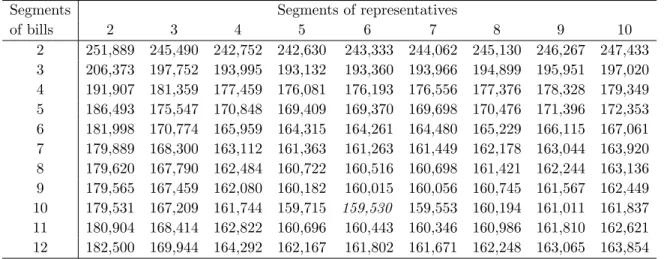
Table 8 displays the AIC-3 values. The lowest AIC-3 value is attained with K = 10 segments of bills and L= 6 segments of representatives; the corresponding log-likelihood value is −66,108.70. For these numbers of segments, we sample an additional 100,000 iterations from the chain that had the highest likelihood value. Due to the large size of the data set, we have no problems with label switching. In the remainder of this section, we present and interpret the results for this model specification.
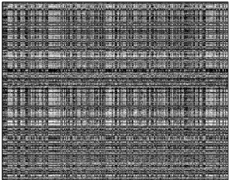
Figure 1: Graphical Representation of Voting Data Set Before (Upper Panel) and After (Lower Panel) Reordering of Rows and Columns. A black box indicates ayea vote and a white box indicates a nay vote.
Representatives Bills 1 100 200 300 400 1 100 200 300 400 500 600 700 Representatives Bills 1 100 200 300 400 1 100 200 300 400 500 600 700
Table 8: AIC-3 values forK = 2, . . . ,12 segments of bills and L= 2, . . . ,10 segments of representatives.
Segments Segments of representatives
of bills 2 3 4 5 6 7 8 9 10 2 251,889 245,490 242,752 242,630 243,333 244,062 245,130 246,267 247,433 3 206,373 197,752 193,995 193,132 193,360 193,966 194,899 195,951 197,020 4 191,907 181,359 177,459 176,081 176,193 176,556 177,376 178,328 179,349 5 186,493 175,547 170,848 169,409 169,370 169,698 170,476 171,396 172,353 6 181,998 170,774 165,959 164,315 164,261 164,480 165,229 166,115 167,061 7 179,889 168,300 163,112 161,363 161,263 161,449 162,178 163,044 163,920 8 179,620 167,790 162,484 160,722 160,516 160,698 161,421 162,244 163,136 9 179,565 167,459 162,080 160,182 160,015 160,056 160,745 161,567 162,449 10 179,531 167,209 161,744 159,715 159,530 159,553 160,194 161,011 161,837 11 180,904 168,414 162,822 160,696 160,443 160,346 160,986 161,810 162,621 12 182,500 169,944 164,292 162,167 161,802 161,671 162,248 163,065 163,854
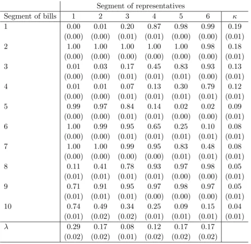
first thing to note is that, except for segments (of bills) 9 and 10, the posterior means of the yea voting probabilities are monotonously increasing or decreasing in each row. For segments 9 and 10, there are only deviations from monotonicity in segment 6 of the representatives. These results imply that the political preferences in the House are one-dimensional. Bills from segment 2 are approved more or less unanimously, and bills from segments 7 and 9 are also widely supported. Bills from other segments seem to be backed by representatives from either segments 1-3 or segments 4-6. In the next subsection, we show that these segments mainly contain Democrats and Republicans, respectively.
To show the effectiveness of our two-mode clustering method, we show graphical repre-sentations of the roll call voting data set before and after reordering the rows and columns according to their segment in Figure 1. For this reordering, we used the segmentation k
and l that yielded the highest likelihood value. Before reordering the rows and columns, it is already apparent that some structure exists in the data; after reordering, the nature of the block structure becomes clear.
5.3
Interpretation of Segments
For each row (bill) and for each column (representative), we compute the marginal poste-rior distribution over the segments. This allow us to compute the means of the explanatory variables within each segment. Table 10 shows the posterior means of the individual
char-Table 9: Posterior means and posterior standard deviations in parentheses of P, κ, and λ. Segment of representatives Segment of bills 1 2 3 4 5 6 κ 1 0.00 0.01 0.20 0.87 0.98 0.99 0.19 (0.00) (0.00) (0.01) (0.01) (0.00) (0.00) (0.01) 2 1.00 1.00 1.00 1.00 1.00 0.98 0.18 (0.00) (0.00) (0.00) (0.00) (0.00) (0.00) (0.01) 3 0.01 0.03 0.17 0.45 0.83 0.93 0.13 (0.00) (0.00) (0.01) (0.01) (0.01) (0.00) (0.01) 4 0.01 0.01 0.07 0.13 0.30 0.79 0.12 (0.00) (0.00) (0.01) (0.01) (0.01) (0.01) (0.01) 5 0.99 0.97 0.84 0.14 0.02 0.02 0.09 (0.00) (0.00) (0.01) (0.01) (0.00) (0.00) (0.01) 6 1.00 0.99 0.95 0.65 0.25 0.10 0.08 (0.00) (0.00) (0.01) (0.01) (0.01) (0.01) (0.01) 7 1.00 1.00 0.99 0.95 0.83 0.48 0.08 (0.00) (0.00) (0.00) (0.00) (0.01) (0.01) (0.01) 8 0.11 0.41 0.78 0.93 0.97 0.98 0.05 (0.01) (0.01) (0.01) (0.01) (0.00) (0.00) (0.01) 9 0.71 0.91 0.95 0.97 0.98 0.97 0.05 (0.01) (0.01) (0.01) (0.00) (0.00) (0.00) (0.01) 10 0.74 0.49 0.34 0.25 0.09 0.15 0.04 (0.01) (0.02) (0.02) (0.01) (0.01) (0.01) (0.01) λ 0.29 0.17 0.08 0.12 0.17 0.17 (0.02) (0.02) (0.01) (0.02) (0.02) (0.02)
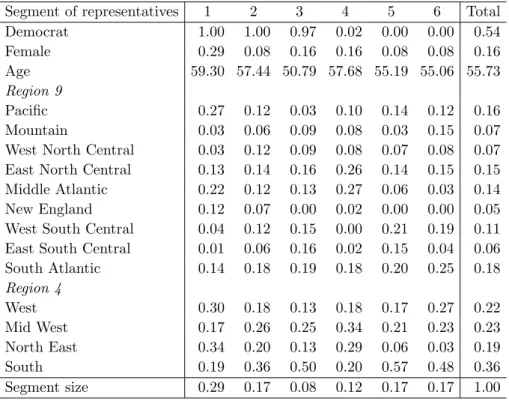
acteristics of the representatives for each segment of representatives. The main result is that the first three segments consist of Democrats, and the last three contain Repub-licans. We know from Table 9 that voting behavior is monotonous; therefore, we can interpret segments 1 and 6 as very partisan Democrats and Republicans, respectively. Segments 2 and 5 seem to be typical Democrats and Republicans, respectively, and the representatives in segments 3 and 4 are relatively moderate. Note that segments 3 and 4 are not completely homogenous, which means that there is a little overlap between these moderate Democrats and Republicans.
Further, we can see that there are relatively more women in the left wing. Not only are women more often Democrats than Republicans, but they also seem to be on the left side within their parties. There appear to be no effects of age within the Republican party, but within the Democratic party, the younger representatives seem to be more moderate
Table 10: Posterior means of individual characteristics for each segment of representatives.
Segment of representatives 1 2 3 4 5 6 Total Democrat 1.00 1.00 0.97 0.02 0.00 0.00 0.54 Female 0.29 0.08 0.16 0.16 0.08 0.08 0.16 Age 59.30 57.44 50.79 57.68 55.19 55.06 55.73 Region 9 Pacific 0.27 0.12 0.03 0.10 0.14 0.12 0.16 Mountain 0.03 0.06 0.09 0.08 0.03 0.15 0.07 West North Central 0.03 0.12 0.09 0.08 0.07 0.08 0.07 East North Central 0.13 0.14 0.16 0.26 0.14 0.15 0.15 Middle Atlantic 0.22 0.12 0.13 0.27 0.06 0.03 0.14 New England 0.12 0.07 0.00 0.02 0.00 0.00 0.05 West South Central 0.04 0.12 0.15 0.00 0.21 0.19 0.11 East South Central 0.01 0.06 0.16 0.02 0.15 0.04 0.06 South Atlantic 0.14 0.18 0.19 0.18 0.20 0.25 0.18 Region 4 West 0.30 0.18 0.13 0.18 0.17 0.27 0.22 Mid West 0.17 0.26 0.25 0.34 0.21 0.23 0.23 North East 0.34 0.20 0.13 0.29 0.06 0.03 0.19 South 0.19 0.36 0.50 0.20 0.57 0.48 0.36 Segment size 0.29 0.17 0.08 0.12 0.17 0.17 1.00
than the older ones.
There are also some clear regional patterns. Representatives from states in the West
are more extreme in their voting behavior, as there are few representatives from these states that are in the moderate clusters 3 and 4. The representatives from thePacific are responsible for the left wing, while the right-wing representatives seem to come mainly from theMountain states. Representatives from theMid West seem to be more moderate than the national average, though this effect is not very strong. In the North East, we find that the Democrats are relatively liberal and that the Republicans are relatively moderate. Finally, in the South, we find that the Democrats are moderate, whereas the Republicans often belong to the most conservative segments.
Table 11 contains the posterior means of the committees for the segments of bills. The results are less pronounced than for the representatives. For example, the posterior means for segment 1 closely resemble the entire sample (that is, the final column in the table), except for the Financial Services committee which is relatively higher.
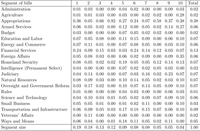
commit-Table 11: Posterior means of committees for each segment of bills.
Segment of bills 1 2 3 4 5 6 7 8 9 10 Total
Administration 0.01 0.03 0.00 0.00 0.04 0.02 0.00 0.00 0.09 0.03 0.02 Agriculture 0.01 0.01 0.03 0.00 0.03 0.00 0.02 0.02 0.00 0.28 0.02 Appropriations 0.36 0.05 0.66 0.92 0.27 0.24 0.07 0.58 0.37 0.38 0.38 Armed Services 0.06 0.05 0.02 0.00 0.12 0.00 0.05 0.02 0.14 0.27 0.06 Budget 0.03 0.00 0.00 0.00 0.07 0.05 0.02 0.02 0.00 0.00 0.02 Education and Labor 0.07 0.05 0.08 0.00 0.11 0.15 0.09 0.00 0.06 0.10 0.07 Energy and Commerce 0.07 0.11 0.01 0.00 0.07 0.08 0.05 0.00 0.03 0.10 0.06 Financial Services 0.24 0.09 0.15 0.03 0.03 0.24 0.14 0.12 0.03 0.07 0.13 Foreign Affairs 0.05 0.08 0.03 0.00 0.06 0.02 0.09 0.00 0.09 0.35 0.06 Homeland Security 0.08 0.05 0.02 0.02 0.19 0.05 0.05 0.12 0.14 0.13 0.07 Intelligence (Permanent Select) 0.04 0.00 0.00 0.00 0.07 0.02 0.02 0.05 0.03 0.00 0.02 Judiciary 0.04 0.14 0.00 0.00 0.07 0.03 0.16 0.02 0.23 0.07 0.07 Natural Resources 0.08 0.09 0.03 0.00 0.10 0.14 0.05 0.02 0.03 0.10 0.07 Oversight and Government Reform 0.03 0.17 0.02 0.00 0.10 0.07 0.14 0.05 0.09 0.10 0.07 Rules 0.01 0.00 0.00 0.00 0.04 0.03 0.00 0.00 0.06 0.03 0.01 Science and Technology 0.04 0.10 0.04 0.01 0.05 0.02 0.09 0.07 0.09 0.10 0.06 Small Business 0.05 0.05 0.01 0.00 0.01 0.02 0.11 0.00 0.00 0.10 0.03 Transportation and Infrastructure 0.06 0.09 0.05 0.03 0.17 0.18 0.15 0.07 0.06 0.10 0.09 Veterans’ Affairs 0.00 0.11 0.00 0.00 0.00 0.00 0.00 0.00 0.00 0.00 0.02 Ways and Means 0.06 0.04 0.00 0.01 0.18 0.11 0.05 0.02 0.11 0.00 0.05 Segment size 0.19 0.18 0.13 0.12 0.09 0.08 0.08 0.05 0.05 0.04 1.00
tee all belong to segment 2, which contains bills that receive nearly unanimous support.
Transportation and Infrastructure is relatively common in segments 5, 6, 7, and 10, which are all primarily favored by Democrats. Bills from theJudiciary committee can primarily be found in segments 2, 7, and 9. For these segments, the voting is almost unanimously
yea. Segment 4 almost solely contains bills from the Appropriations committee. Only the hard-line Republicans from segment 6 vote in majority (79%) yea for these bills. To a lesser extent, this is also true for bills from segment 3, though there is a little more support for these bills, even from some of the moderate Democrats in segment 3.
6
Conclusions
We have developed a Bayesian approach to do inference in a latent-class two-mode cluster-ing model, which has several advantages over frequentist parameter estimation methods. First, our method allows for statistical inference on the model parameters, which is not possible using a maximum likelihood approach. Furthermore, the Bayesian approach also
allows us to do statistical inference on the number of segments using marginal likelihoods. An alternative way to select the numbers of segments is to consider information criteria. The third advantage of using Bayesian techniques is that fewer computational problems occur during parameter estimation.
We have applied our model to the Supreme Court voting data set of Doreian et al. (2004). The marginal likelihoods used to determine the optimal number of segments indicate fewer segments than were found in these previous studies. In the second example, we consider roll call votes from the United States House of Representatives in 2007. We detect six segments of representatives and ten segments of bills. Three of the individual segments contain Democrats and the other three segments contain Republicans, though there is a little overlap. We also find clear regional effects on voting behavior.
Finally, our approach can easily be extended in several directions. First, it can easily be adopted to use with data matrices with arbitrary distributions. Although we have only derived posterior samplers for Bernoulli and normally distributed data, it is straight-forward to derive posterior samplers for all kinds of distributions. Secondly, our method can easily be extended to three-mode data, see Schepers, Van Mechelen, and Ceulemans (2006). Thirdly, explanatory variables can be added, either with segment-dependent ef-fects or as concomitant variables, that is, variables explaining why a row (or column) belongs to a certain segment, see Dayton and MacReady (1988) and Wedel (2002) for a discussion.
References
Andrews, R. L., & Currim, I. S. (2003). A comparison of segment retention criteria for finite mixture logit models. Journal of Marketing Research,40, 235-243.
Berger, J. (1985). Statistical decision theory and Bayesian analysis. New York: Springer-Verlag.
Bozdogan, H. (1994). Mixture-model cluster analysis using model selection criteria and a new information measure of complexity. In H. Bozdogan (Ed.),Proceedings of the first US/Japan conference on the frontiers of statistical modeling: An informational approach (Vol. 2, p. 69-113). Boston: Kluwer.
Brusco, M., & Steinley, D. (2006). Inducing a blockmodel structure of two-mode binary data using seriation procedures. Journal of Mathematical Psychology,50, 468-477. Candel, M. J. J. M., & Maris, E. (1997). Perceptual analysis of two-way two-mode
fre-quency data: Probability matrix decomposistion and two alternatives. International Journal of Research in Marketing,14, 321-339.
Celeux, G., Hurn, M., & Robert, C. P. (2000). Computational and inferential difficulties with mixture posterior distributions. Journal of the American Statistical Associa-tion, 95, 957-970.
Davies, R. B. (1977). Hypothesis testing when a nuisance parameter is present only under the alternative. Biometrika, 64, 247-254.
Dayton, C. M., & MacReady, G. B. (1988). Concomitant variable latent class models.
Journal of the American Statistical Association,83, 173-178.
De Leeuw, J. (2006). Principal component analysis of binary data by iterated singular value decomposition. Computational Statistics & Data Analysis, 50, 21-39.
Dempster, A. P., Laird, N. M., & Rubin, D. B. (1977). Maximum likelihood estimation from incomplete data via the EM algorithm.Journal of the Royal Statistical Society, Series B, 39, 1-38.
DeSarbo, W. S., Fong, D. K. H., Liechty, J. C., & Saxton, M. K. (2004). A hierarchical Bayesian procedure for two-mode cluster analysis. Psychometrika,69, 547-572. Dias, J. G., & Wedel, M. (2004). An empirical comparison of EM, SEM and MCMC
per-formance for problematic Gaussian mixture likelihoods. Statistics and Computing,
14, 323-332.
Doreian, P., Batagelj, V., & Ferligoj, A. (2004). Generalized blockmodeling of two-mode network data. Social Networks, 26, 29-53.
Fraley, C., & Raftery, A. E. (1998). How many clusters? Which clustering method? Answers via model-based cluster analysis. The Computer Journal,41, 578-588. Fr¨uhwirth-Schnatter, S. (2001). Markov chain Monte Carlo estimation of classical and
dynamic switching and mixture models. Journal of the American Statistical Asso-ciation,96, 194-209.
switching models using bridge sampling techniques. Econometrics Journal,7, 143-167.
Fr¨uhwirth-Schnatter, S. (2006). Finite mixture and Markov switching models. New York: Springer.
Gelman, A., Carlin, J. B., Stern, H. S., & Rubin, D. B. (2003). Bayesian data analysis. Chapman & Hall.
Geman, S., & Geman, D. (1984). Stochastic relaxation, Gibbs distributions, and the Bayesian restoration of images. IEEE Transactions on Pattern Analysis and Ma-chine Intelligence, 6, 721-741.
Geweke, J. (2007). Interpretation and inference in mixture models: Simple MCMC works.
Computational Statistics & Data Analysis, 51, 3529-3550.
Govaert, G., & Nadif, M. (2003). Clustering with block mixture models. Pattern Recog-nition,36, 463-473.
Govaert, G., & Nadif, M. (2008). Block clustering with Bernouilly mixture models: Comparison of different approaches. Computational Statistics & Data Analysis,52, 3233-3245.
Han, C., & Carlin, B. P. (2001). Markov chain Monte Carlo methods for computing Bayes factors: A comparative review. Journal of the American Statistical Association,96, 1122-1133.
Hartigan, J. A. (1975). Clustering algorithms. New York: John Wiley and Sons.
Hartigan, J. A. (2000). Bloc voting in the united states senate. Journal of Classification,
17, 29-49.
Heckman, J. J., & Snyder Jr., J. M. (1997). Linear probability models of the demand for attributes with an empirical application to estimating the preferences of legislators.
RAND Journal of Economics, 28, S142-S189.
Kass, R. E., & Raftery, A. E. (1995). Bayes factors. Journal of the American Statistical Association, 90, 773-795.
Milligan, G. W., & Cooper, M. C. (1985, June). An examination of procedures for determining the number of clusters in a data set. Psychometrika,50(2), 159-179. Nelson, J. P. (2002). “green” voting and ideology: LCV scores and roll-call voting in the
U.S. senate, 1988-1998. The Review of Economics and Statistics, 84, 518-529. Newton, M. A., & Raftery, A. E. (1994). Approximate Bayesian inference by the weighted
likelihood bootstrap. Journal of the Royal Statistical Society, Series B, 56, 3-48. Poole, K. T., & Rosenthal, H. (1991). Patterns of congressional voting. American Journal
of Political Science, 35, 228-278.
Schepers, J., Ceulemans, E., & Mechelen, I. van. (2008). Selecting among multi-mode partitioning models of different complexities: A comparison of four model selection criteria. Journal of Classification, 25, 67-85.
Schepers, J., Van Mechelen, I., & Ceulemans, E. (2006). Three-mode partitioning. Com-putational Statistics & Data Analysis, 51, 1623-1642.
Symons, M. J. (1981). Clustering criteria and multivariate normal mixtures. Biometrics,
37, 35-43.
Tanner, M. A., & Wong, W. H. (1987). The calculation of posterior distributions by data augmentation. Journal of the American Statistical Association, 82, 528-540. Tierney, L. (1994). Markov chains for exploring posterior distributions. Annals of
Statis-tics, 22(4), 1701–1762.
Van Mechelen, I., Bock, H. H., & De Boeck, P. (2004). Two-mode clustering methods: A structured overview. Statistical Methods in Medical Research, 13, 363-394.
Van Rosmalen, J., Groenen, P. J. F., Trejos, J., & Castillo, W. (2009). Optimization strategies for two-mode partitioning. Journal of Classification, forthcoming.
Wedel, M. (2002). Concomitant variables in finite mixture models. Statistica Neerlandica,
56, 362-375.
Wedel, M., & Kamakura, W. A. (2000). Market segmentation: Conceptual and method-ological foundations (second ed.). Boston: Springer.