Complex-Valued Time-Series Correlation Increases Sensitivity in FMRI Analysis

(1)

Mathematics, Statistics and Computer Science

Faculty Research and Publications

Mathematics, Statistics and Computer Science,

Department of

7-1-2016

Complex-Valued Time-Series Correlation

Increases Sensitivity in FMRI Analysis

Mary C. Kociuba

Marquette University

Daniel B. Rowe

Marquette University, [email protected]

Accepted version.

Magnetic Resonance Imaging, Vol. 34, No. 6 ( July 2016): 765-770.

DOI. © 2016

Elsevier. Used with permission.

NOTICE: this is the author’s version of a work that was accepted for publication in Magnetic

Resonance Imaging. Changes resulting from the publishing process, such as peer review, editing,

corrections, structural formatting, and other quality control mechanisms may not be reflected in this

document. Changes may have been made to this work since it was submitted for publication. A

definitive version was subsequently published in Magnetic Resonance Imaging, VOL. 34, ISSUE 6,

July 2016,

DOI.

(2)

Magnetic Resonance Imaging, Vol. 34, No. 6 (July 2016): pg. 765-770. DOI. This article is © Elsevier and permission has been granted for this version to appear in e-Publications@Marquette. Elsevier does not grant permission for this article to be further copied/distributed or hosted elsewhere without the express permission from Elsevier.

1

Complex-Valued Time-Series

Correlation Increases Sensitivity in

FMRI Analysis

Mary C. Kociuba

Department of Mathematics, Statistics, and Computer Science,

Marquette University

Milwaukee, WI

Daniel B. Rowe

Department of Mathematics, Statistics, and Computer Science,

Marquette University

Department of Biophysics, Medical College of Wisconsin

Milwaukee, WI

Abstract

Purpose: To develop a linear matrix representation of correlation between

complex-valued (CV) time-series in the temporal Fourier frequency domain, and demonstrate its increased sensitivity over correlation between

magnitude-only (MO) time-series in functional MRI (fMRI) analysis.

Materials and methods: The standard in fMRI is to discard the phase before

the statistical analysis of the data, despite evidence of task related change in the phase time-series. With a real-valued isomorphism representation of Fourier reconstruction, correlation is computed in the temporal frequency domain with CV time-series data, rather than with the standard of MO data. A MATLAB simulation compares the Fisher-z transform of MO and CV

(3)

2

amplitude change in the time-series. The increased sensitivity of the complex-valued Fourier representation of correlation is also demonstrated with

experimental human data. Since the correlation description in the temporal frequency domain is represented as a summation of second order temporal frequencies, the correlation is easily divided into experimentally relevant frequency bands for each voxel's temporal frequency spectrum. The MO and CV correlations for the experimental human data are analyzed for four voxels of interest (VOIs) to show the framework with high and low contrast-to-noise ratios in the motor cortex and the supplementary motor cortex.

Results: The simulation demonstrates the increased strength of CV

correlations over MO correlations for low magnitude contrast-to-noise time-series. In the experimental human data, the MO correlation maps are noisier than the CV maps, and it is more difficult to distinguish the motor cortex in the MO correlation maps after spatial processing.

Conclusions: Including both magnitude and phase in the spatial correlation

computations more accurately defines the correlated left and right motor cortices. Sensitivity in correlation analysis is important to preserve the signal of interest in fMRI data sets with high noise variance, and avoid excessive processing induced correlation.

Keywords: Magnetic resonance imaging; Functional magnetic resonance

imaging; Frequency correlation; Complex correlation

1. Introduction

In fMRI, the measured blood oxygen level dependent (BOLD) signal to detect neural activity is spatially Fourier encoded [1] and [2]. The BOLD fluctuations are measured as a complex-valued fMRI signal over time in the spatial frequency domain, then the k-space readout is reconstructed with the inverse Fourier transform (IFT). Before the statistical analysis of the fMRI data, the phase portion of the data is generally discarded, despite physiologically useful information contained in the phase [3]. Previous research suggests that phase-only change arises from large draining vessels [4], or proposes methods to filter phase signal contributions from large vessels

[4] and [5]. Although, other models support the notion that randomly oriented vasculature yield phase change in fMRI studies [6] and [7]. It has been previously demonstrated that modeling an fMRI time-series with both magnitude and phase increases the power of the activation statistics [8], [9], [10] and [11] over those from MO models. This manuscript outlines a method to describe correlation between two time-series with both magnitude and phase (equivalently real and imaginary), through exploiting the linear relationship between the image domain and spatial frequency domain. Traditionally both MO

(4)

3

and CV models require analysis in the image domain, however,

analysis within the frequency domain is also valuable. It has previously been shown how complex-valued temporal frequencies contribute to the correlations between voxels in the cerebral cortex for magnitude-only non-task data [12]. Similarly, in this manuscript the spatial correlation between complex-valued time series is described as a linear combination of second order voxel temporal frequencies. The present study advances the frequency correlation description into a linear matrix framework with an application to a complex-valued simulation demonstrating the strength of the model at low magnitude and phase contrast-to-noise ratio (CNR) values, as well demonstrating its utility in experimental complex-valued fMRI data.

During signal acquisition, unwanted image acquisition artifacts and physiological noise obscure the true underlying signal of interest. To improve the signal-to-noise ratio (SNR), various preprocessing operations, i.e. temporal frequency filtering or magnitude image smoothing, are incorporated in the processing and reconstruction pipeline, and physiologic noise sources are commonly regressed out from the signal [13], [14], [15] and [16]. It is well documented that the application of these operations induces local spatial and temporal correlations into neural regions that were previously uncorrelated [17], [18] and [19]. The linear framework developed in this manuscript also describes how signal processing alters the structure of the spatial covariance matrix, such that induced correlation is a result of increased overlapping frequency content between voxels after

processing. Signal processing will alter the activated voxel's temporal frequency spectrums, by spreading voxel task activated peaks

temporally and spatially. Correlation will be induced between voxels as a result of increased overlapping frequency content between the two voxel's Fourier frequency spectrums. This notation for spatial

correlation is advantageous since various physiological signals are also confined to specific frequency ranges. Respiratory and cardiac cycle fluctuations are characterized around 0.2–0.3 Hz and 1 Hz in a voxel's temporal frequency spectrum, although they are often aliased to low frequencies in fMRI signal acquisition [13], [20] and [21]. The

summation notation of spatial correlation that is described here, allows relative contributions to the correlation to be quantified by segregating the natural partitions in a voxel's temporal frequency spectrum.

(5)

4

with complex-valued data more accurately identifies regions of spatial correlation, and reduces the false positives in correlation maps. This result is most significant in low magnitude CNR data sets since including the phase in the complex-valued correlation results in increased sensitivity of identifying correlated regions.

2. Theory

A prow × pcol complex-valued k-space readout is reconstructed to

a single image with the discrete inverse Fourier transform (IFT). With a real-valued isomorphism representation [22] of the Fourier

reconstruction operator, Ω, and the k-space readout in vector form, st,

an image vector, yt, for a single image time point, t, is reconstructed

as

y

_t

= Ω

_S_t

equation(1) Equivalently, with the forward Fourier Transform Ω− 1₌

_Ω

̅

_{, the}

k-space readout is written as

S

_t

= Ω

̅y

_t

,

equation(2) In Eqs. (1) and (2), the signal and image vectors are 2p × 1, where p = prowpcol is the number of voxels, and the real parts are

stacked over the imaginary parts, so st = (sR’,sI’)’ and yt = (yR’,yI’)’.

The real parts in each vector are organized as sR = (sR1,…,sRp)’ and

yR = (yR1,…,yRp)’, and the imaginary parts in each vector are organized

as sI = (sI1,…,sIp)’ and yI = (yI1,…,yIp)’. To build up the real-valued

matrix framework, consider the representation of the inverse Fourier reconstruction.

𝛺 = [

𝛺

_𝛺

𝑅

−𝛺

𝐼

𝛺

𝑅

]

where ΩR and ΩI are constructed with the Kronecker product,

(6)

5

and ΩI = [(ΩyR⊗ ΩxI) + (ΩyI⊗ ΩxR)]. The jkth element of the

pcol × pcol Fourier matrix Ωx is (Ωx)jk = w (pcol₂ + j) (pcol₂ + k) where j and

k have indexing values from 0 to pcol − 1 with w = _𝑁1𝑒𝑖2𝜋⁄𝑃𝑐𝑜𝑙 for the IFT

and w = e–i2π/p_col_{for the forward Fourier transform (FT), [22].}

To reconstruct images over n time repetitions (TRs), the

complex-valued spatial frequencies are represented in the real-valued 2pn × 1 vector s, with each successive TR concatenated to the vector. An analogous explanation describes the organization of the real-valued image 2pn × 1 vector, y, which is reconstructed with the Kronecker product,

y = (I

_n

⨂Ω)s

equation(3) A 2pn × 2pn permutation matrix, P, reorders the elements of vector y so the real-valued time-series 2pn × 1 vector v = Py is now ordered by voxel rather than ordered by image. The voxel ordered time-series is Fourier transformed into the temporal frequency domain, with the 2n × 2n temporal forward Fourier transform (FT) matrix, 𝛺𝑇,

as opposed to the 2p × 2p spatial Fourier operations. The real-valued 2pn × 1 vector f consists of the temporal frequencies of each voxel stacked upon the corresponding imaginary temporal frequencies is represented,

𝑓 = (I

_p

⨂Ω

̅

_Τ

)Py

equation(4) For voxel α, the 2n × 1 real-valued voxel time-series is denoted vα, with real parts stacked over imaginary parts vα = (vαR’,vαI’)’ so the

real and imaginary parts in each vector are organized as

vαR = (vαR1,…,vαRn)’ and vαI = (vαI1,…,vαIn)', with a mean and covariance

structure of μRα and μIα., σ2RαIn and σ2IαIn.The corresponding temporal

frequencies for voxel α are denoted in the 2n × 1 vector fα, where

vα = ΩTfα and fα = ΩTvα, are organized similarly to the time-series

equivalent. With an analogous description of another voxel β, the spatial covariance between the two voxels is simply written, cov(vα,

(7)

6

Assuming the time-series is demeaned, then the covariance between two voxels in terms of temporal frequencies is represented as,

cov(

v

_α

, v

_β

)

=

(

v

Τ_α

v

_β

) (

⁄

2n

)

=

(

Ω

̅

_Τ

𝑓

_α

)

Τ

(

Ω

̅

_Τ

𝑓

_β

)

=

(

𝑓

_αΤ

𝑓

_β

)

⁄ 4

equation(5) The spatial covariance in Eq. (5) is expanded to a p × p spatial covariance matrix, Σ, such that the entry (α, β) in Σ represents the spatial covariance between the two demeaned real-valued voxel time-series of voxel α and voxel β. By defining D as the diagonal matrix consisting of the diagonal elements of Σ, a p × p spatial correlation matrix is written as,

R = D

−½

_∑D

−½

equation(6) By aggregating the second order temporal frequencies into biologically meaningful or experimentally relevant bands, the influence preprocessing steps have on each voxel temporal frequency spectrum can be quantitatively measured. In an fMRI study, the frequency corresponding to the activation is considered when dividing the spectrum into bands. To understand the contribution each temporal frequency band yields to spatial correlation, the correlation is

expressed as, the spatial covariance matrix can be written as a summation of covariance of each band and b is the total number of bands,

𝛴 = 𝛴

₁

+ ⋯ + 𝛴

_𝑏

,

and the Eq. (7) spatial correlation matrix can be written as a summation of correlation of bands

R = D − ½(Σ

₁

+ ⋯ + Σ

_b

)D − ½ = R

₁

+ ⋯ + R

_b

equation(7) Input of processing operations in the context of the Fourier framework is described in Appendix A.

(8)

7

3. Methods

3.1. Theoretical illustration

To demonstrate the improved strength of correlation between CV time-series over correlation between MO time series in functional MRI studies, a MATLAB simulation is run with a varying degree of magnitude contrast-to-noise ratio (CNRρ) and the phase

contrast-to-noise ratio (CNRϕ). The SNR is defined as the baseline magnitude

signal over the standard deviation of the noise in the time-series, SNR = ρ/σ. For the CNR, the amplitude is defined as the difference between the baseline signal and the task related change in the signal for the magnitude and phase components of the time-series, Aρ and

Aϕ, so CNRρ = Aρ/σ and CNRϕ = Aϕ/(σ/ρ). Assuming normal noise in the

real and imaginary channels, the standard deviation of a phase-only time-series is σ/ρ, and the CNRϕ is proportional to the SNR. Typically

in fMRI studies, the task related signal change in the magnitude Aρ

corresponds to approximately a 1–2% signal change, and the task related change in the phase Aϕ has been found to be approximately

π/36 [4]. To compare MO and CV correlations, two 96 × 96 surfaces are generated with 720 time-points and standard normal random noise added to the real and imaginary channels. As visualized in Fig. 1, each voxel has a ρ between 0 and 50, and a task generated to represent a magnitude amplitude Aρ between 0 and 1, and a phase amplitude Aϕ

between 0 and π/36. The MO and CV correlations are computed

between the two time-series in each surface with equivalent parameter settings, so there is a 96 × 96 corresponding matrix for MO and CV. To compare the correlations between the two models, the Fisher-z

transform, z, is computed and plotted for each time-series correlation, r, as

𝑧 = ½ ln (

1 + 𝑟

1 − 𝑟

)

(9)

8

Fig. 1. Surfaces representing the (a) ρ, (b) Aρ, and (c) Aϕ parameters used to

generate the simulated time-series.

3.2. Experimental illustration

An experimental fMRI human data set is acquired with bilateral finger tapping, performed for sixteen 22-s periods, a block design experiment was acquired for a series of 720 TRs with a 3.0 T

Discovery MR750 MRI scanner (General Electric, Milwaukee, WI) using a GE single channel quadrature head coil. The data set was acquired with ten interleaved 4 mm thick axial slices that are 96 × 96 in

dimension for a 24.0 cm FOV, with a TR/TE of 1000/39 ms, a flip angle of 25°, and an acquisition bandwidth of 111 kHz. To observe the

potential impact of data processing on the temporal frequencies and demonstrate the utility of the framework, voxel temporal spectrums are analyzed before and after applying a spatial smoothing operator with a Gaussian kernel with a full-width-half-max of 3 voxels, followed by an ideal high-pass band filter (< 0.009 Hz) and low-pass band filter (> 0.08 Hz). The spatial correlation is decomposed into three

correlation bands, R1, R2, R3, such that sum of the bands equals the

total correlation. The correlation bands that are selected correspond to the frequency band ranges 0.0009–0.024 Hz, 0.026–0.037 Hz, 0.038– 0.08 Hz, with the task-activated frequency peak is observed in R2. The

complex activation for the data was computed [9], and four voxels were chosen based on their complex activation locations: two in the motor cortex and two in the supplementary motor cortex. The two voxels in each location are chosen so that one voxel has a high CNRρ

(10)

9

4. Results

4.1. Simulated data

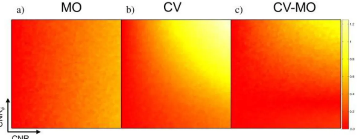
In Fig. 2, the Fisher-z transform statistics for the MO and CV correlations are computed for the surfaces generated with the

parameters described in Fig. 1. Including the phase half of the data in the CV correlation calculation yields an increased sensitivity of the correlation value, as illustrated by comparing the top left corner of the Fisher-z map in Fig. 2a to the one in Fig. 2b, with a difference map of CV–MO in Fig. 2c. The additional information of the phase time-series improves the strength of correlation detected at lower magnitude CNR values.

Fig. 2. The Fisher-z transform of the (a) MO and (b) CV correlation, and the (c)

difference (CV–MO) between the correlations.

4.2. Experimental data

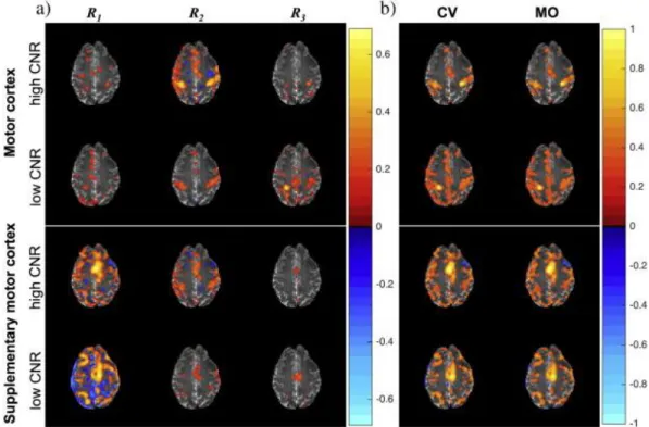
Fig. 3 and Fig. 4 contain the four seed voxel CV and MO spatial correlation maps for the experimental fMRI data in the motor cortex and supplementary motor cortex. In Fig. 3b, the MO and CV

correlation maps are identical since computing the MO and CV

correlations are equivalent for a MO data set. In Fig. 4b, the MO and CV correlation maps are noticeably distinguishable since computing the MO and CV correlations are not equivalent for a CV data set. As

described in Eq. (7), the spatial correlations are computed with the temporal frequencies, which are aggregated into bands as seen in Figs. 3a and 4a. The MO correlation maps appear to contain more

(11)

10

correlations outside the expected task-activated region compared to the CV maps. Particularly in the low CNR seed voxels, the less defined motor cortex in the MO correlation maps corroborates the results observed in the simulation in Section 4.1. The CV correlations have a higher sensitivity than the MO correlations in both regions with

activation. All voxels are located in the motor cortex or supplementary motor cortex, and exhibit task-activated correlation in R2, where the

task frequency peak is located, as in Figs. 3a and 4a. In Fig. 3b, the general location of the apparent false positive MO correlation is around the edge of the brain as is characteristic of a motion artifact. Since the data has been minimally processed, motion artifacts are present in the data and have not been corrected.

Fig. 3. Experimental MO fMRI spatial correlation maps for each seed voxel (a) by the

correlation bands, R1, R2, R3 corresponding to the frequency band ranges 0.0009– 0.024 Hz, 0.026–0.037 Hz, 0.038–0.08 Hz, and (b) the total correlation map CV and MO for high and low CNR in motor cortex and supplementary motor cortex.

(12)

11

Fig. 4. Experimental CV fMRI spatial correlation maps for each seed voxel (a) by the

correlation bands, R1, R2, R3 corresponding to the frequency band ranges 0.0009– 0.024 Hz, 0.026–0.037 Hz, 0.038–0.08 Hz, and (b) the total correlation map CV and MO for high and low CNR in motor cortex and supplementary motor cortex.

5. Conclusions

A linear matrix representation of correlation between complex-valued time-series in the temporal Fourier frequency domain for functional MRI (fMRI) data analysis was developed. In a simulation comparing decreasing CNR magnitude and phase values, it was illustrated that the Fisher-z transform of CV correlations was higher than for MO correlations for low CNR fMRI time-series. In the

experimental human data, a comparison of R2 in Figs. 3a and 4a shows

increased sensitivity of estimating correlations with including the phase time-series. These results agree with previous studies investigating the statistical power of using CV data over MO data in fMRI studies. In comparison to the MO correlations, the CV correlations have reduced error, and more distinctive regions of activation in the motor cortex and the supplementary motor cortex for voxels with lower magnitude and phase CNR. While the framework is demonstrated for task fMRI data, a natural application of this framework is to non-task fMRI,

(13)

12

where the spatial correlation is measured to detect long-range connectivity.

The temporal Fourier frequency description in this study is also advantageous to locate the temporal frequency range where

correlations are induced. Common processing and reconstruction methods have been shown to induce correlation of no biological origin [18], [23] and [24]. In this study a framework is presented where signal processing operations and parallel image reconstruction procedures, applied to the complex-valued k-space signal, can be represented as real-valued matrix operators. The second order

temporal frequency spatial covariance representation describes spatial correlation as a function of increased overlapping frequency content. Consider a scenario where initially voxel a and b are correlated, b and c are correlated, but a and c are not correlated. If the reconstructed images are smoothed, which have been previously shown to induce correlation, spatial correlation between a and b arises from

overlapping frequency content between temporal frequency spectrums of a and c. Similar reasoning can be used to discuss the correlation between b and c, and the lack of correlation between a and c. As shown in Appendix A, the matrix multiplication of the linear operators with the spatial covariance matrix, quantitatively describes the

compounding impact of spatial and temporal operators to the second order temporal frequencies. Combining this matrix multiplication framework with biologically or experimentally relevant frequency bands pertaining to fMRI data, provides insight into the impact of signal processing on statistical analysis and clinical interpretations from the data. The application of the theory to complex-valued data validates the increased statistical strength of using complex-valued models, specifically in minimally processed data sets or data sets with high noise variability. Including the phase in the analysis increases the sensitivity of the correlation in low magnitude contrast-to-noise ratio functional MRI data.

Acknowledgements

(14)

13

Appendix A.

A linear matrix representation of the spatial covariance and correlation, allows one to measure the effect of the temporal and spatial processing operators. Define a p × p spatial smoothing operator, Sm, which filters the real and imaginary components

separately with a Gaussian kernel. Continuing the notation used in Eq. (3) with a demeaned time-series notation, the smoothed 2pn × 1 temporal frequency vector is constructed with the multiplication vs = (Ip⊗ Τ)P(I2n ⊗ Sm)y.

The series of operations applied to the temporal frequencies is defined with 2pn × 2pn operator,

O = (I2n ⊗ Sm)P(Ip ⊗ T) such that the 2pn × 1 unprocessed and

processed time-series vectors ordered by voxel are represented as in Eqn. (3), y = (Ip ⊗ T)v and ys = Ov. The 2pn × 2pn spatiotemporal

covariance matrix for the 2pn × 1 real-valued image time-series, y, in terms of temporal frequency spectrum, is defined as

cov[y] = Γ,

equation(A.1) and the covariance matrix with processing operators is defined

cov[y

_s

] = ΟΓΟ

´

_.

equation(A.2) Eqs. (A.1) and (A.2) are described in terms of temporal

frequencies as shown in Section 2.1. The spatial component of Eq. (A.1) is equivalent to Σ described in Eq. (5), through a process of summing real and imaginary diagonal values to achieve a sp × p magnitude-squared spatial correlation matrix such that the temporal component is held constant. Magnitude-squared correlation is

(15)

14

References

[1] P.A. Bandettini, E.C. Wong, R.S. Hinks, R.S. Tikofsky, J.S. Hyde. Time course EPI of human brain function during task activation. Magn Reson

Med, 25 (1992), pp. 390–397

[2] S. Ogawa, T.M. Lee, A.R. Kay, D.W. Tank. Brain magnetic resonance imaging with contrast dependent on blood oxygenation. Proc Natl Acad

Sci U S A, 87 (1990), pp. 9868–9872

[3] F.G. Hoogenraad, P.J. Pouwels, M.B. Hofman, J.R. Reichenbach, M. Sprenger, E.M. Haacke. Quantitative differentiation between BOLD models in fMRI. Magn Reson Med, 45 (2001), pp. 233–246

[4] R.S. Menon. Postacquisition suppression of large-vessel BOLD signals in high-resolution fMRI. Magn Reson Med, 47 (2002), pp. 1–9

[5] A.S. Nencka, D.B. Rowe. Reducing the unwanted draining vein BOLD contribution in fMRI with statistical post-processing methods.

Neuroimage, 37 (2007), pp. 177–188

[6] F. Zhao, T. Jin, P. Wang, X. Hu, S.G. Kim. Sources of phase changes in BOLD and CBV-weighted fMRI. Magn Reson Med, 57 (2007), pp. 520– 527

[7] Z. Feng, A. Caprihan, K.B. Blagoev, V.D. Calhoun. Biophysical modeling of phase changes in BOLD fMRI. Neuroimage, 47 (2) (2009), pp. 540– 548

[8] D.B. Rowe, B.R. Logan. A complex way to compute fMRI activation.

Neuroimage, 23 (2004), pp. 1078–1092

[9] D.B. Rowe. Modeling both the magnitude and phase of complex-valued fMRI data. Neuroimage, 25 (2005), pp. 1310–1324

[10] D.B. Rowe. Magnitude and phase signal detection in complex-valued fMRI data. Magn Reson Med, 62 (2009), pp. 1356–1357

[11] S.K. Arja, Z. Feng, Z. Chen, A. Caprihan, K.A. Kiehl, T. Adali, et al. Changes in fMRI magnitude data and phase data observed in block-design and event-related tasks. Neuroimage, 49 (2010), pp. 3149– 3160

[12] D. Cordes, V.M. Haughton, K. Arfanakis, J.D. Carew, P.A. Turski, M.A. Quigley, et al. Frequencies contributing to functional connectivity in the cerebral cortex in “resting-state” data. Am J Neuroradiol, 22 (2001), pp. 1326–1333

[13] R.M. Birn, J.B. Diamond, M.A. Smith, P.A. Bandettini. Separating respiratory-variation-related fluctuations from neuronal-activity-related fluctuations in fMRI. Neuroimage, 31 (2006), pp. 1536–1548 [14] G.H. Glover, T.Q. Li, D. Ress. Image-based method for retrospective

correction of physiological motion effects in fMRI: RETROICOR. Magn

(16)

15

[15] A.D. Hahn, A.S. Nencka, D.B. Rowe. Enhancing the utility of complex-valued functional magnetic resonance imaging detection of

neurobiological processes through post acquisition estimation and correction of dynamic B0 errors and motion. Hum Brain Mapp, 33

(2012), pp. 288–306

[16] X. Hu, T.H. Le, T. Parrish, P. Erhard. Retrospective estimation and correction of physiological fluctuation in functional MRI. Magn Reson

Med, 34 (1995), pp. 201–212

[17] K.J. Friston, O. Josephs, E. Zarahan, A.P. Holmes, S. Rouquette, J.B. Poline. To smooth or not to smooth? Bias and efficiency in fMRI time-series analysis. Neuroimage, 12 (2000), pp. 196–208

[18] A.S. Nencka, A.D. Hahn, D.B. Rowe. A mathematical model for

understanding statistical effects of k-space (AMMUST-k) preprocessing on observed voxel measurements in fcMRI and fMRI. J Neurosci

Methods, 181 (2009), pp. 268–282

[19] C.E. Davey, D.B. Grayden, G.F. Egan, L.A. Johnston. Filtering induces correlation in fMRI resting state data. Neuroimage, 64 (2013), pp. 728–740

[20] P.K. Bhattacharyya, M.J. Lowe. Cardiac-induced physiologic noise in the tissue is a direct observation of cardiac-induced fluctuations. Magn

Reson Imaging, 22 (2004), pp. 9–13

[21] K. Shmueli, P. van Glederen, J.A. de Zwart, S.G. Horovitz, M. Fukunaga, J.M. Jansma, et al. Low-frequency fluctuation in the cardiac rate as a source of variance in the resting-state fMRI BOLD signal. Neuroimage, 38 (2007), pp. 306–320

[22] D.B. Rowe, A.S. Nencka, R.G. Hoffmann. Signal and noise of Fourier reconstructed fMRI data. J Neurosci Methods, 159 (2007), pp. 361– 369

[23] I.P. Bruce, M.M. Karaman, D.B. Rowe. A statistical examination of the SENSE reconstruction via an isomorphism representation. Magn Reson

Imaging, 29 (2011), pp. 1267–1287

[24] I.P. Bruce, D.B. Rowe. Quantifying the statistical impact of GRAPPA in fcMRI data with a real-valued isomorphism. IEEE Trans Med Imaging, 33 (2014), pp. 495–503

[25] D.B. Rowe, A.S. Nencka. Induced correlation In FMRI magnitude data from k-space preprocessing. Proc Int Soc Magn Reson Med, 17 (2009), p. 1721

Corresponding author at: Department of Mathematics, Statistics, and

Computer Science, Marquette University, Milwaukee, WI, USA. Tel.: + 1 414 288 5228; fax: + 1 414 288 5472.