Targeted Maximum Likelihood Estimation of Natural Direct Effect

(1)

University of California, Berkeley

U.C. Berkeley Division of Biostatistics Working Paper Series

Year  Paper

Targeted Maximum Likelihood Estimation of

Natural Direct Effect

Wenjing Zheng

∗

Mark J. van der Laan

†

∗_{Division of Biostatistics, University of California, Berkeley, wenjing.zheng@ucsf.edu} †_{Division of Biostatistics, University of California, Berkeley, laan@berkeley.edu}

This working paper is hosted by The Berkeley Electronic Press (bepress) and may not be commer-cially reproduced without the permission of the copyright holder.

http://biostats.bepress.com/ucbbiostat/paper288 Copyright c2011 by the authors.

(2)

Targeted Maximum Likelihood Estimation of

Natural Direct Effect

Wenjing Zheng and Mark J. van der Laan

Abstract

In many causal inference problems, one is interested in the direct causal effect of an exposure on an outcome of interest that is not mediated by certain inter-mediate variables. Robins and Greenland (1992) and Pearl (2000) formalized the definition of two types of direct effects (natural and controlled) under the coun-terfactual framework. Since then, identifiability conditions for these effects have been studied extensively. By contrast, considerably fewer efforts have been in-vested in the estimation problem of the natural direct effect. In this article, we propose a semiparametric efficient, multiply robust estimator for the natural direct effect of a binary treatment using the targeted maximum likelihood framework of van der Laan and Rubin (2006) and van der Laan and Rose (2011). The proposed estimator is asymptotically unbiased if either one of the following holds: i) the conditional outcome expectation given exposure, mediator, and confounders, and the mediated mean outcome difference are consistently estimated; (ii) the expo-sure mechanism given confounders, and the conditional outcome expectation are consistently estimated; or (iii) the exposure mechanism given confounders, and a ratio of conditional mediator densities are consistently estimated. Moreover, case (iii) implies in particular that estimation of the conditional mediator den-sity may be replaced by consistent estimation of the exposure mechanism and the conditional distribution of exposure given confounders and mediator. If all three conditions hold, then the effect estimate is asymptotically efficient.

(3)

1 Introduction

The causal effect of an exposure (ortreatment) on an outcome of interest is often times mediated by intermediate variables (mediator). In many causal inference problems, one is interested in the direct effect of such exposure on the outcome, not mediated by the effect of the intermediate variables. Robins and Greenland (1992) and Pearl (2000) defined two types of direct effects under the counterfactual framework. The

controlled direct effect refers to the effect of the exposure on the outcome under an idealized experiment where the mediator is set to a given constant value, whereas the

natural (or pure) direct effect pertains to an experiment where the mediator is set to be distributed according to the null exposure level and the individual’s covariates. The definition of these causal effects are based on counterfactual outcomes that are not fully observed, therefore they are not always identifiable from the observed data. Identifiability conditions are studied extensively in Robins and Greenland (1992), Pearl (2000), Robins (2003), van der Laan and Petersen (2004), Hafeman and Van-derWeele (2010), Imai et al. (2010), and Pearl (2011).

Prior to the formal frameworks developed by Robins and Greenland (1992) and Pearl (2000), the social science literature had proposed the use of parametric linear structural equations in mediation analysis (e.g. Baron and Kenny (1986)), where the outcome response and mediator response are each modeled using linear main term regression on their parent nodes, and the direct and indirect effects are defined and estimated in terms of coefficients in these regression equations. The limited causal validity of this parameter due to its dependence on model specification (e.g. no-interactions and linearity assumptions) is discussed in Kaufman et al. (2004). The developments of Robins and Greenland (1992) and Pearl (2000), and the identifiability studies that followed suit, address definition and identification of direct and indirect effects in a framework that is detached from statistical model specifications, allowing one to separate the identification problem from the estimation problem.

Several approaches to the estimation problem are available in the current litera-ture. A likelihood-based estimator approach (the g-computation formula) builds upon the identifiability results using a substitution estimator plugging in maximum likeli-hood based estimates of the relevant components of the data generating distribution. The natural direct effect may be identified as a function of the marginal covari-ate distribution, the conditional mediator distribution, conditioned on null exposure and individual covariates, and the conditional outcome distribution, conditioned on exposure, mediator and individual covariates (Robins and Greenland (1992), Pearl (2000), Robins (2003) and van der Laan and Petersen (2004)). When all of these components of the data generating distribution are estimated consistently, the re-sulting g-computation estimate is unbiased and efficient. However, if either of these components is inconsistent, the effect estimate will be biased. VanderWeele and Vansteelandt (2010) illustrated how this approach may be applied to the estima-tion of natural direct effect odds ratio of rare outcomes. The use of (sequential) g-computation in structural nested models for estimation of controlled direct effects is proposed in Vansteelandt (2009). A second approach to causal effects estimation is based on the estimating function methodology developed by Robins (1999), Robins

(4)

and Rotnitzky (2001) and van der Laan and Robins (2003), where the root to a score equation is used as the effect estimate. For most parameters arising from missing data problems (including causal effect parameters), the efficient score under a nonparamet-ric model is a robust estimating function (i.e. unbiased against mis-specification of the missingness mechanism or mis-specification of the full data model), therefore the resulting effect estimate shares the same robustness properties. In van der Laan and Petersen (2008), an application of this approach to a generalized class of direct effects using marginal structural models was discussed. The parameter studied in that work is a population mean of a subject-specific average controlled direct effect, averaged with respect to a user-specified conditional mediator density given null exposure and individual covariates. If the supplied conditional mediator density is the true condi-tional mediator density of the data generating process, then the parameter of van der Laan and Petersen (2008) evaluates to the same value as the natural direct effect parameter. However, even in such case, these two parameters are not the same maps on the model since the former is a map indexed by the supplied mediator density and is a function of the outcome expectation and marginal covariate distribution alone. As a consequence, the efficient score of the parameter of van der Laan and Petersen (2008) is not the same as the efficient score of the natural direct effect parameter we study in this article. VanderWeele (2009) discussed more fully the use of marginal structural models with inverse probability weighting for estimation of the natural direct effect parameter. Most recently, Tchetgen Tchetgen and Shpitser (2011) devel-oped the application of the estimating function methodology to natural direct effect estimation using the efficient score equation, as well as a sensitivity analysis frame-work for the assumption of ignorability of the mediator variable. We also refer the interested reader to their work for discussion on semiparametric efficiency bounds for the nonparametric model. A third approach to causal effect estimation is the targeted maximum likelihood framework of van der Laan and Rubin (2006) and van der Laan and Rose (2011). For each relevant component of the data generating distribution, one obtains a loss-based estimate that would solve the corresponding component of the efficient score equation. These estimates are then used to obtain a substitution estimator of the parameter of interest. The resulting estimator solves the efficient score equation, therefore also shares its robustness properties. In addition, the sub-stitution principle allows for estimation of the parameter range providing additional information gain, and preserves properties of the parameter as a map on the model. van der Laan and Petersen (2008) also applied the targeted MLE procedure to their generalized class of direct effect parameters. Both the estimating function approach and the targeted MLE approach in van der Laan and Petersen (2008) are robust (with respect to its parameter of interest) against mis-specification of the conditional ex-pected outcome or mis-specification of the treatment mechanism. However, since its parameter of interest is indexed by the user-supplied conditional mediator density, if one is interested in the natural direct effect, then the user-specified conditional medi-ator density in the method of van der Laan and Petersen (2008) must be correct. The use of propensity score matching in estimation of causal effects from observational studies was introduced in Rosenbaum and Rubin (1983). Application of propensity score in mediation analysis has also been proposed (e.g. Jo et al. (2011)).

(5)

In this article, we apply the targeted MLE framework of van der Laan and Rubin (2006) and van der Laan and Rose (2011) to the estimation of the natural direct ef-fect of a binary exposure. The identifiability results in Robins and Greenland (1992), Pearl (2000), Robins (2003) and van der Laan and Petersen (2004) imply in particular that the natural direct effect of a binary treatment may be estimated as the marginal mean (over strata of confounders) of the mediated mean outcome difference, where the mediated mean outcome difference is the conditional expectation of the difference in outcome under two different exposure levels, conditioned with respect to the medi-ator given null exposure and confounders. We propose a semiparametric efficient and robust estimator which, given initial estimators of the exposure mechanism, condi-tional mediator density and condicondi-tional outcome expectation, targetedly modifies the estimates of the conditional outcome expectation and the mediated mean outcome difference using a set of parametric working submodels. These resulting targeted components are then used to produce a plug-in estimator for the parameter of in-terest. The procedure systematically incorporates estimation of the boundary of the parameter domain. The set of parametric working submodels are defined such that the resulting estimator solve the efficient score equation, and hence inherits its robust-ness properties. The proposed estimator is asymptotically unbiased if either one of the following holds: i) the conditional outcome expectation, and the mediated mean outcome difference are consistently estimated; (ii) the exposure mechanism given con-founders, and the conditional outcome expectation are consistently estimated; or (iii) the exposure mechanism given confounders, and a ratio of conditional mediator den-sities are consistently estimated. If all three conditions hold, then the effect estimate is asymptotically efficient.

This article is organized as follows: In section 2 we define formally the natural direct causal effect of a binary treatment on an outcome using the Non-Parametric Structural Equations Model framework of Pearl (2009), and summarize its identifi-ability conditions. Based on the identifiidentifi-ability result, one may consider the natural direct effect parameter as a map from the model to the parameter space. We study this map in greater detail in section 2.3. In particular, the robustness properties of its efficient score under a nonparametric model are summarized in lemma 1 of that section. Section 3 begins with a general description of the targeted MLE estima-tion framework of van der Laan and Rubin (2006), and then presents a step by step construction of the targeted MLE estimator for the natural direct effect of a binary treatment. Asymptotic properties of this estimator are summarized in section 3.2 and proved in the Appendix A. The estimation procedure in section 3 focuses on the targeted estimation of the conditional outcome expectation and the mediated mean outcome difference, as described above. An alternative procedure focusing on the conditional outcome expectation and the conditional mediator density is described in Appendix B. This alternative estimator shares the same asymptotic properties as the one proposed in section 3. Section 4 describes in greater detail two alternative esti-mators under the estimation equation framework of Robins (1999), and the maximum likelihood based g-computation framework. In section 5, we illustrate with simula-tions the robustness of the targeted MLE estimator against model mis-specificasimula-tions. We will also explore the performance of the various estimators in the presence of data

(6)

sparsity. This article concludes with a summary.

2 Natural Direct Effect of a binary treatment

2.1 Causal Parameter

Consider n i.i.d observations of O = (W, A, Z, Y), where W represents baseline co-variates, A a binary treatment, Z represents the mediator between the treatment and the outcome of interest Y. Let P0 denote the distribution of O. We apply here

the Non-Parametric Structural Equations Model of Pearl (2009) to encode the causal relations of interest. The NPSEM on an unit consists of a set of exogenous random variables U which are determined by factors outside the model, a set of endogenous variables X which are determined by variables inside the system (U ∪X), and a set of unspecified deterministic functions{fx :x∈X}which encodes for each x∈X the

variables that have direct influence on x. More specifically, in the present situation the causal relations are encoded by the NPSEM

U = (UW, UA, UZ, UY)∼PU

W = fW(UW)

A = fA(W, UA)

Z = fZ(W, A, UZ)

Y = fY(W, A, Z, UY),

whereX = (W, A, Z, Y) is the endogenous variable, and U = (UW, UA, UZ, UY) is the

unobserved exogenous variable. This model defines a random variable (U, X) on the unit of observation, we denote its distribution by PU,X.

One may define a submodel of the NPSEM by intervening on a subset of the equations. The counterfactual variables or potential outcomes in the Rubin Causal Model (Rubin (1978), Rosenbaum and Rubin (1983) and Holland (1986)) may then be interpreted as variables in the post-intervention submodel. For instance, the coun-terfactualZ(a) is defined as the random variable Z in a system where one intervened to set Z = fZ(W, a, UZ), and may be interpreted as the mediator variable that the

unit would have had if the exposure had been a. Similarly, Y(a0, Z(a)) is the coun-terfactual outcome that results from setting Y = fY(W, a0, Z(a), UY), and may be

interpreted as the response that one may have had if the exposure had been a0 while the mediator variable had been identical to the one under exposurea.

Under the NPSEM, a causal parameter of interest may be defined as a function of the distribution PU,X. More specifically, thenatural direct causal effect is defined

as

Ψ(PU,X) = E[Y(1, Z(0))−Y(0, Z(0))].

This causal parameter may be interpreted from the following hypothetical randomized trial: one randomly assigns each subject to treatment or control, while setting the subject’s mediator variable to be distributed as if treatment was absent, and then take the difference in mean outcome between the treated and control cohort.

(7)

2.2 Identifiability

Under experimental or observational studies, for each unit the investigator only ob-serves the outcome and mediating response under the unit’s actual exposure, that is,

O = (W, A, Z(A), Y(A, Z(A)). Hence, the causal parameter Ψ(PU,X) is not always

identifiable from the observed data.

Conditions under which the natural direct effect will be identifiable are addressed extensively in Robins and Greenland (1992), Pearl (2000), Robins (2003), van der Laan and Petersen (2004), Hafeman and VanderWeele (2010), Imai et al. (2010), and Pearl (2011). In particular, if the randomization assumptions

1. For all values (a, z), (A, Z) is independent ofY(a, z), given W; 2. For all values of a, A is independent of Z(a), given W;

and the conditional independence assumption

3. For all z,E(Y(1, z)−Y(0, z)|Z(0) =z, W) = E(Y(1, z)−Y(0, z)|W)

are satisfied, then the causal effect Ψ(PU,X) may be expressed as a function of the

observed data generating distribution P0:

Ψ(P0) =EW ( X z [E(Y|W, A= 1, Z =z)−E(Y|W, A= 0, Z=z)]p(z|W, A= 0) ) . (1)

In the following sections, we will focus on the estimation of this statistical parameter. The randomization assumptions 1 and 2 ensure that sufficient covariates are mea-sured to control for confounding of the effects of treatment on outcome, treatment on mediator, and mediator on outcome. As a result, the counterfactual elementsY(a, z) and Z(a) will be identifiable within covariate stratum. Under these randomization assumptions alone, the statistical parameter (1) equals the population mean of a subject-specific average controlled direct effectP

z(Y(1, z)−Y(0, z))P(Z(0) =z|W)

(van der Laan and Petersen (2008)). Therefore, in the absence of the conditional independence assumption 3 the statistical parameter (1) still offers a causal interpre-tation.

2.3 The Natural Direct Effect parameter

Let Mdenote a model containing the true data generating distribution P0. For any

P ∈ M, the likelihood decomposes into

P(O) = PW(W)PA(A|W)PZ(Z|W, A)PY(Y|W, A, Z).

For later convenience, we adopt the notations g(A|W, Z) = PA(A|W, Z), QW(W) =

PW(W), QZ(Z|W, A) = PZ(Z|W, A), and ¯QY(W, A, Z) = E(Y|W, A, Z). Moreover,

let Q = (QW, QZ,Q¯Y). The notations Q0 and g0 are reserved for the corresponding

components of the true data generating distributionP0. For a functionf(O), we will

use P f to denote the expectation off(O) under the probability distributionP ∈ M.

(8)

For instance, P0f ≡ P_o∈Of(o)dP0(o) denotes the expectation of f under the true

data generating distribution, while Pnf ≡ _n1 P_in₌₁f(oi) is the empirical mean off.

One may consider the natural direct effect parameter Ψ as a map

Ψ : M → R P 7→ Ψ(P) = Ψ(Q)≡EQW EQZ Q¯Y(W,1, Z)−Q¯Y(W,0, Z)|W, A= 0 . The parameter of interest in (1) is thus

ψ0 ≡Ψ(P0) = EQW,0

EQZ,0 Q¯Y,0(W,1, Z)−Q¯Y,0(W,0, Z)|W, A= 0

.

We refer to the inner expectation above as the(null level) mediated mean outcome difference, and denote it by

EQZ( ¯QY|W,0)≡ X z ¯ QY(W,1, z)−Q¯Y(W,0, z) QZ(z|W,0). (2)

This mediated difference is a function of W alone. For convenience, we may abuse the notation EQZ( ¯QY) ≡ EQZ( ¯QY|W,0) when referring to the function of W. This

way, Ψ(P) = Ψ QW, EQZ( ¯QY)

.

Effcient score

Under a nonparametric model M, for any P ∈ M, the efficient score (efficient influence curve, or canonical gradient) of Ψ at P is given by

D∗(Q, g,Ψ(Q)) = _I₍_A_{= 1)} g(1|W) QZ(Z|W,0) QZ(Z|W,1) −I(A= 0) g(0|W) Y −Q¯Y(W, A, Z) +I(A= 0) g(0|W) _¯ QY(W,1, Z)−Q¯Y(W,0, Z)−EQZ Q¯Y(W,1, Z)−Q¯Y(W,0, Z)|W,0 +EQZ Q¯Y(W,1, Z)−Q¯Y(W,0, Z)|W,0 −Ψ(Q) =D_Y∗ +D_Z∗ +D_W∗ .

Note that the components D∗_Y, D_Z∗, D∗_W are respectively the projection of D∗ onto the tangent subspaces corresponding to the components P(Y|W, A, Z), P(Z|W, A),

P(W) of the likelihood.

This efficient score for a nonparametric model may be derived by first considering Ψ(P) as a function of P = (P f : f ∈ F), where F is a class of indicator functions

F = {I(w, a, z, y), I(w, a, z), I(w, a), I(w) : w ∈ W, a ∈ {0,1}, z ∈ Z, y ∈ Y}. For any given ”vector” h = (h(f) :f ∈ F), one may consider a directional derivative

d

dΨ(P +h)|=0. The efficient score is then given by the directional derivative

ap-plied to the direction of h = (f(O)−P f :f ∈ F). In other words, it is given by

P

f∈F

∂Ψ(P)

∂Pf (f(O)−P f). A more detail exposition may be found in van der Laan

and Rose (2011).

Lemma 1. Robustness of the efficient score

Suppose there exists 1 > δ > 0 such that g(A = 1|W) <1−δ a.e. over the support of W. The efficient score is a robust estimating function for the parameter at P0, in

the sense that

P0D∗(Q, g, ψ0) = 0

if either of the following holds:

(9)

(i) The conditional outcome expectation Q¯Y = E(Y|W, A, Z), and the mediated

mean outcome difference EQZ Q¯Y,0(W,1, Z)−Q¯Y,0(W,0, Z)|W,0

are correct. (ii) The treatment mechanismg =p(A|W), and the conditional outcome expectation

¯

QY =E(Y|W, A, Z) are correct.

(iii) The treatment mechanism g = p(A|W), and the conditional mediator density ratio QZ(Z|W,0)/QZ(Z|W,1)are correct.

(iv) The treatment mechanismg =p(A|W), and the conditional distribution of treat-ment given mediator and covariates p(A|W, Z) are correct.

The proof of this lemma is straightforward, and we refer the interested reader to Appendix A. A noteworthy observation is that in case (i), it was not necessary that

QZ =QZ,0. But rather, any functionEZ( ¯QY,0|W,0) which captures the dependence of

the true outcome difference on the null exposure and confounder, and equals the true mediated mean differenceEQZ,0( ¯QY,0|W,0) will yield the desired result. This suggests

that in the case where the outcome expectation can be correctly estimated while the treatment mechanism and the mediator density are difficult to ascertain, one may still obtain unbiasedness using a consistent data-adaptive estimator that regresses the correctly predicted outcome difference onW among the control observations. On the contrary, in cases when g is correct, robustness does not impose any requirement on

EQZ( ¯QY|W,0). In fact, the cancelation in the proof shows that it may be any function

of W. We illustrate this last observation in the simulation section (implemented as TMLE 2). Case (iv) is a simple consequence of case (iii). In situations when Z is high dimensional, consistent estimation ofp(A|W, Z) may prove more attainable than consistent estimation of QZ(Z|W, A).

It is worthwhile to note that in the case where only ¯QY is correctly specified, the

solution ψ1 to the equation P0D∗( ¯QY,0, QZ, g, ψ) = 0 corresponds to an alternative

effect parameter of the form ψ1 = EW,0 ( X z ¯ QY,0(W,1, z)−Q¯Y,0(W,0, z) × (QZ,0(z|W,0)−QZ(z|W,0)) g0(0|W) g(0|W) +QZ(z|W,0) ) = ψ0 + EW,0 ( X z ¯ QY,0(W,1, z)−Q¯Y,0(W,0, z) × (QZ,0(z|W,0)−QZ(z|W,0)) _g 0(0|W) g(0|W) −1 )

(10)

3 Targeted MLE for the Natural Direct Effect of

a binary treatment

In general, under the framework of van der Laan and Rubin (2006) the construction of a targeted estimator of a parameter of interest Ψ(P0) calls for two sets of ingredients.

For each componentQj of Q, one defines a uniformly bounded (w.r.t. the supremum

norm) loss function Lj :Qj → L∞(K) satisfying

Qj,0 = arg min

Qj∈Qj

P0Lj(Qj),

whereL∞₍_K_{) is the class of functions of} _O _{with bounded supremum norm over a set}

of K containing the support of O under P0. Given the loss functionLj, one defines a

one-dimensionalparametric working submodel {Qj(Q, g, ) :} ⊂ M passing through

Q at= 0 with score D_j∗(Q, g) at = 0 that satisfies

hd

dLj(Qj(Q, g, ))|=0i ⊃ hD

∗

j(Q, g)i. (3)

The acceptable functional forms of the submodel are thus ruled by the loss function

Lj and the functional form ofD∗j. The loss functions and their respective parametric

submodels satisfying (3) allow for loss-based estimates of each components ofQ that would also solve the corresponding component of the efficient score equation.

To specialize to the natural direct effect, we first note that the parameter of interest and the components D∗_Z and D_W∗ of the efficient score depend on QZ only through

the mediated mean outcome difference EQZ( ¯QY) as denoted in (2). Secondly, the

empirical marginal distribution ˆQW ofW is a consistent estimator ofQW,0that readily

solves the equationPnD∗W(EQZ( ¯QY),QˆW) = 0 for anyEQZ( ¯QY). Hence, the proposed

estimator will focus on targeted estimation of ¯QY,0(W, A, Z), andEQZ,0( ¯QY,0|W,0).

An alternative targeted estimation to the one proposed above is to targetedly es-timate the conditional mediator density QZ,0 instead of the mediated mean outcome

difference EQZ,0( ¯QY,0|W,0). We refer the interested reader to Appendix B for this

alternative approach. The proposed and the alternative targeted procedures both require an initial estimator of the conditional mediator densityQZ,0. Their key

differ-ence lies in that the former defines a loss function and parametric working submodel for the mediated mean outcome differenceEQZ( ¯QY|W,0), whereas the latter defines a

loss function and parametric working submodel for the conditional mediator density

QZand then estimates the mediated mean outcome difference plugging in the targeted

mediator density and the targeted ¯QY. The bias-variance trade-off in the targeting

step of the first approach is more optimal for estimating the ultimate component of interest, which is the mediated mean outcome difference.

3.1 Construction of the targeted MLE

Loss functions

Suppose Y is binary or continuous and bounded. In the latter case, without loss of generality we may assume that Y is bounded in (0,1). In this case, a valid loss

(11)

function for ¯QY is the minus-loglikelihood

LY( ¯QY)(O) =−

Y log ¯QY(W, A, Z) + (1−Y) log(1−Q¯Y(W, A, Z)) . (4)

For a given ¯QY(·), suppose ¯QY(W,1, Z)−Q¯Y(W,0, Z) is also bounded. Without

loss of generality, we may also assume it’s bounded between (0,1). Let the loss function for EQZ( ¯QY|W,0) be LZ(EQZ( ¯QY))(O) = −I(A= 0)× n ¯ QY(W, A, Z) logEQZ( ¯QY|W,0) + (1−Q¯Y(W, A, Z)) log(1−EQZ( ¯QY|W,0)) o . (5)

Linear transformations onto the unit interval may be needed in order to use loss functionsLY andLZ. However, since the parameter of interest and the components of

the efficient score are linear in ¯QY andEQZ( ¯QY), the necessary linear transformations

and their inverse maps do not affect the properties of the estimators.

In a more general setting one may instead use the squared error loss functions

LY( ¯QY)(O) = Y −Q¯Y(W, A, Z) 2 , and LZ(EQZ( ¯QY))(O) = Q¯Y(W, A, Z)−EQZ( ¯QY|W,0) 2 I(A = 0).

Parametric working submodels.

Under the loss function (4) for ¯QY, consider the logistic working submodel

¯ QY(QZ, g)(1)≡expit logit( ¯QY) +1CY(QZ, g) , where CY(QZ, g)(O) = n I(A=1) g(1|W) QZ(Z|W,0) QZ(Z|W,1) − I(A=0) g(0|W) o

. This submodel satisfies

d d1 LY Q¯Y(QZ, g)(1) |1=0=D ∗ Y( ¯QY, QZ, g). (6)

Similarly, for a given EQZ( ¯QY|W,0), under the loss function (5) the logistic

work-ing submodel EQZ( ¯QY)(g)(2)≡expit logit(EQZ( ¯QY)) +2CZ(g) , with CZ(g)(O) = _g_(0|1_W₎, satisfies d d2 LZ EQZ( ¯QY)(g)(2) |2=0=D ∗ Z(EQZ( ¯QY),Q¯Y, g). (7)

In the case where the squared error loss function is used, the parametric working submodels are of the form

¯

QY(QZ, g)(1) = ¯QY +1CY(QZ, g)

and

EQZ( ¯QY)(g)(2) =EQZ( ¯QY) +2CZ(g).

(12)

Implementation

Let Pn denote the empirical distribution of n i.d.d observations of O. Let ˆQ¯Y, ˆQZ,

and ˆg be respectively initial estimators of ¯QY,0, QZ,0 and g0. Let

ˆ 1∗ = arg min PnLY ˆ ¯ QY( ˆQZ,gˆ)(1)

be the optimal 1 which minimizes the empirical risk. The update

ˆ ¯

Q∗_Y ≡Qˆ¯Y( ˆQZ,gˆ)(ˆ∗) (8)

is the targeted MLE estimator of Q¯Y,0.

Next, let ˆEZ( ˆQ¯∗Y|W,0) be an initial estimator of the mediated mean outcome

difference EQZ,0

ˆ ¯

Q∗_Y(W,1, Z)−Qˆ¯∗_Y(W,0, Z) | W, A = 0. This may be constructed using a plug-in estimator with ˆQZ and ˆQ¯∗Y. The optimal 2 is given by

ˆ 2 ∗ = arg min PnLZ ˆ EZ( ˆQ¯∗Y)(ˆg)(2) . The update ˆ E_Z∗( ˆQ¯∗_Y)≡EˆZ( ˆQ¯∗Y)(ˆg)( ∗ 2) (9)

is thetargeted MLE estimator ofEQZ,0

ˆ ¯ Q∗_Y(W,1, Z)−Q¯ˆ∗_Y(W,0, Z)|W, A= 0 . More-over, it is a function ofW alone, i.e. ˆE_Z∗( ˆQ¯∗_Y|W,0) = ˆE_Z∗( ˆQ¯∗_Y)(W). The targeted MLE estimator of ψ0 is thus given by

ˆ ψ∗ = 1 n n X i=1 ˆ E_Z∗( ˆQ¯∗_Y)(Wi). (10)

It follows from (6) thatPnDY∗( ˆQ¯∗Y,QˆZ,ˆg) = 0 and it follows from (7) thatPnD∗Z

ˆ

E_Z∗( ˆQ¯∗_Y),Qˆ¯∗_Y,gˆ

= 0. Moreover, the empirical distribution ˆQW of W solves PnD∗W( ˆE

∗

Z( ˆQ¯

∗

Y),QˆW) = 0.

Therefore the resulting targeted estimator solves the efficient score equation.

Remarks on implementation

When Z is high dimensional, consistent estimation of p(A|W, Z) may be more at-tainable than consistent estimation of QZ(Z|W, A). In such case, instead of using an

estimator of QZ to estimate the ratio QZ(Z|W,0)/QZ(Z|W,1) in the targeting step

of ¯QY, one may use an estimator pˆ_g(_ˆA₍_A=0|_=0|W,z_w₎)_p_ˆˆg₍(_AA_=1|=1|_W,zW)₎.

In the step of targeting the mediated mean outcome difference, we mentioned the plug-in estimator using the initial mediator density and the targeted outcome pre-dictor as an initial estimator. However, the initial estimator may be any function

EZ( ˆQ¯∗Y|W,0) of W which regresses the predicted outcome difference given by ˆQ¯

∗

Y

on W among control observations. From lemma 1, we see that when the treatment mechanism is correct, i.e. in cases (ii), (iii), and (iv), the specification of the me-diated mean outcome difference per se does not affect robustness (we illustrate this observation using implementation TMLE 2 in the simulations section).

(13)

3.2 Asymptotic Properties of the Targeted MLE

Since the proposed targeted MLE estimator solves the efficient score equation, lemma 1 implies in particular that the estimator is asymptotically unbiased if either of the following is true: (i) The conditional outcome expectation ˆQ∗_Y and the mediated mean outcome difference ˆE_Z∗( ˆQ¯∗_Y|W,0) are consistent; (ii) the treatment mechanism ˆg and the conditional outcome expectation ˆQ¯∗_Y are consistent; (iii) the treatment mechanism

g, and the conditional mediator density ratioQZ(Z|W,0)/QZ(Z|W,1) are consistently

estimated. These properties are illustrated in the simulations section below.

Under certain empirical conditions, an estimator that solves an estimating equa-tion will be asymptotically linear with influence curve given by the estimating func-tion (e.g.. van der Vaart (1998), van der Laan and Robins (2003), Tsiatis (2006), Kosorok (2008)). In such case, central limit theorem implies that one may obtain an asymptotic variance estimate of the said estimator using the variance estimate of its influence curve. We detail conditions for asymptotic linearity of the targeted MLE estimator in the theorem 1 in Appendix A.

Empirical process conditions are often necessary for the asymptotic linearity of an Z-estimator as they restrict the size of the class of functions containing the influence curve (we refer to the CV-TMLE framework in Zheng and van der Laan (2010) and Zheng and van der Laan (2011) for an alternative targeted estimator which avoids such conditions through the use of cross-validation). The conclusion (18) of theorem 1 shows that under certain empirical process conditions, the estimator behaves as an empirical mean of mean zero i.i.d. random variables (which converges to a normal distribution by CLT), plus specified second order remainders from which one may infer the conditions needed for asymptotic linearity.

When true treatment mechanism g0 is used in the estimation procedure (e.g. in

an RCT), the remainders concerning estimation of g0 vanish, leaving only a second

order remainder term which concerns the speed at which the targeted outcome expec-tation estimator ˆQ¯∗_Y and the initial mediator density ˆQZ converge to their respective

limits, and two first order remainder terms concerning the difference between these limits and the truth. Asymptotic linearity requires firstly that the second order term be oP(1/

√

n) (condition (19) of theorem 1). If both ˆQ¯∗_Y and ˆQZ are consistent (and

satisfies this speed condition), then the estimator is asymptotically linear. Moreover, if the plug-in initial estimator for the mediated mean outcome difference is used in this case, it follows that the estimator is in fact asymptotically efficient. Otherwise, asymptotic efficiency follows only if the initial estimator of the mediated mean out-come difference is also consistent. In the case that one of the two components, ¯QY or

QZ, is inconsistently estimated, the resulting first order remainder will have to satisfy

an asymptotically linear condition ((23) or (21)). This implies in particular that if one uses a data-adaptive estimator for the outcome ¯QY,0, then the estimator ˆQZ,n for

the mediator density needs to converge fast enough so that second order condition (19) is satisfied. Even though this compromise may cause the mediator density es-timator to be inconsistent, as long as the outcome eses-timator ˆQ∗_Y,n is consistent and satisfies the asymptotic linearity condition of (21), then the effect estimate will still

(14)

be asymptotically linear. On the other hand, if one chooses to use a data-adaptive estimator for the mediator density, it may come at the expensive of a smaller model for the outcome so that (19) is met. If this smaller model for the outcome is not correct, then the mediator density estimator will need to be consistent and satisfy the asymptotically linear condition of (23).

When the true treatment mechanismg0is not used, one is confronted with 3 second

order remainders that concern the speeds at which the pairs

ˆ ¯ Q∗_Y,QˆZ , ˆ ¯ Q∗_Y,gˆ , and ˆ

g,Eˆ_Z∗( ˆQ¯∗_Y)converge to their respective limits, and 3×2 = 6 first order remainders that concern the difference between these limits and the truth. Asymptotic linearity requires firstly that the 3 second order remainders areoP(1/

√

n) (conditions (19), (25) and (26) ). This impose restrictions on how large a model one may use to estimate each component. If g0 is contained in a correctly specified parametric model (e.g. it only

depends on a discrete covariate and one uses a saturated model), then rate conditions (25) and (26) are satisfied for reasonable estimators of ¯QY,0andQZ,0. However, ifg0is

contained in a large semiparametric model, the estimators for outcome and mediator density will need to both converge fast enough so that conditions (25) and (26) are satisfied, which severely restrict their data-adaptiveness. If all the components are consistently estimated, then the effect estimator is asymptotically efficient. However, if one of the components is inconsistent, then one is confronted with two first order remainders and asymptotic linearity conditions on these terms are needed to ensure asymptotic linearity of the resulting effect estimate.

In short, asymptotic linearity requires that (a) estimators of each component con-verge to their respective limits at a reasonable speed; (b) at most one component may be inconsistently estimated, in which case the consistent estimators of the remaining components must meet stricter asymptotic linearity conditions.

More generally, many conditions which concern estimation of the mediator density are in fact conditions on estimation of the mediator density ratio (as we see in theorem 1). Therefore, if one decides to make use of case (iv) in lemma 1, the estimation of

p(A|W, Z) ought to be such that the corresponding speed conditions and first-order linearity conditions are satisfied for the resulting mediator density ratio estimator.

4 Some existing estimation methodologies

In this section, we describe how the estimating equation approach and the g-computation approach may be applied to the natural direct effect of a binary exposure, and contrast their theoretical properties with those of the proposed targeted estimator.

4.1 Estimating equation approach

Under the estimating equation based approach (Robins (1999), Robins and Rotnitzky (2001), van der Laan and Robins (2003)), one may use the efficient score under a nonparametric model as the estimating function. An estimate of the parameter is given by a root of the efficient score equation. In missing data and causal inference

(15)

applications, where the observed data is regarded as a ’censored’ version of a full data structure, the efficient score of a parameter of the observed data distribution will involve inverse weighting of the treatment (censoring) mechanism. Moreover, the efficient score is an unbiased estimating function if either the relationship between outcome and covariates under the full data model or the treatment mechanism is correct. Therefore, this approach is also known as doubly robust inverse probability treatment (or censoring) weighting (DR-IPTW).

Under this framework, an estimate for the natural direct effect is given by solving for the root of the equation given by the efficient score in section 2.3. We refer to Tchetgen Tchetgen and Shpitser (2011) for detailed study of this estimator. For given estimators ˆQY, ˆQZ, ˆEZ( ˆQ¯Y) and ˆg, the natural direct effect estimate is given by

By design, this estimator solves the efficient score equation

PnD∗ ˆ QY,QˆZ,EˆZ( ˆQ¯Y),ˆg,ψˆdriptw = 0.

Therefore, the DR-IPTW estimator and the proposed targeted MLE estimator share the same asymptotic properties that are inherited from the efficient score. By the same token, they are both sensitive to extreme values of the treatment model, such as in the case of near positivity violations. This was demonstrated in Kang and Schafer (2007). Indeed, in the case of natural direct effect, when ˆg(Ai|Wi) is small for some

observations, the estimated D∗_Y component of the efficient score will be large; this problem is exacerbated if Ai = 0, in which case the estimated DZ∗ is also large.

When near positivity violation is present, the estimating equation estimator may yield estimates that are out of the bounds of the parameter. For instance, in the case of binary outcome Ψ is the mean difference of two probabilities and hence bounded between -1 and 1. But under extreme values ofPnDˆ∗Y andPnDˆ∗Z, the DR-IPTW may

yield estimates that are out of these bounds. The proposed targeted estimator using a logistic working submodel (introduced in Gruber and van der Laan (2010)) aims to provide more stable estimates through the combination of a unit linear transfor-mation, which estimates implicitly the boundary of the parameter domain, and the virtue of a substitution estimator, which effectively translates domain boundary into bounds of the parameter range.

4.2 G-computation approach

The sensitivity to near positivity violation of the targeted estimator and the DR-IPTW estimator stem from the use of inverse probability weightings in the efficient score. A g-computation approach based on the identifiability result in (1) avoids this inverse weighting. More specifically, for ˆQY and ˆQZ likelihood based estimators of

(16)

the outcome expectation and mediator density, respectively, consider a g-computation estimator given by:

ˆ ψgcomp = 1 n n X i=1 ˆ QY(Wi,1, Zi)−QˆY(Wi,0, Zi) ˆ QZ(Zi|Wi,0).

Unlike the robustness of the targeted estimator and the DR-IPTW estimator, the consistency of the g-computation estimator relies on correct specification of both the outcome expectation and mediator density. In the case of these likelihood-based estimates being correct, the resulting ˆψgcomp is more efficient than the two robust

estimators. However, even though this g-computation estimator does not use inverse probability weighting explicitly, it may still be affected by the data sparsity, since quality of the outcome expectation estimate (even under the correct model) is sensitive to the overlap between the empirical covariate distribution of the treated and the empirical covariate distribution of the control.

5 Simulation Study

In this section we evaluate the performance of the targeted estimator, the DR-IPTW estimator, and the g-computation estimator under model mis-specification and data sparsity. From lemma 1, one expects to see that in the absence of positivity violations, the TMLE and DR-IPTW be robust against model mis-specifications.

5.1 Simulation schemes

The following three data generating schemes are used. The mediator variable Z

is discrete with three categories, i.e. Z ∈ {0,1,2}. Each scheme has a version with a binary outcome Y and a version with a continuous and bounded outcome Y. Simulations 2 and 3 differ from simulation 1 in their mediator density and treatment mechanism, respectively.

(17)

1. Simulation 1: no positivity violations. W ∼U(0,2) A∼Bern expit(−1 + 2W −0.08W2) Z ∼M ultinom p(Z = 0) =expit(−0.2 + 0.5A+ 0.3A×W+ 0.7W−1.5W2), p(Z= 1|Z 6= 0) =expit(−0.2 + 0.4A+.8A×W+ 0.4W −2.5W2) ! versiona: Y ∼Bern expit(−2 +A−W+W2+Z+ 0.8A×W −A×W2 −0.5A×Z+ 0.7A×Z2) ! versionb: Y ∼ −0.1 + 0.5A−0.2W+ 0.1W2+ 0.2Z+ 0.4A×W−0.5A×W2 −0.3A×Z+ 0.5A×Z2+N(0,1)

Probability of receiving treatment give covariate, gA(A = 1|w), is bounded

in (0.26,0.94). Probability of a particular mediator value z given A = 1 and

W = w, QZ(z|A = 1, w), is bounded between (0.0005,0.9753), whereas the

ratio QZ(z|A = 0, w)/QZ(z|A = 1, w) for a particular z and w is bounded

in (0.1376,2.0103). In version b with continuous outcome, the expected value

E(Y|W, A, Z) is bounded in (−0.8,2.25).

The parameters of interest are ψ0 = 0.2585079 for the binary version, and

ψ0 = 1.158052 for the continuous version. The semiparametric efficiency bounds

are var(D∗(P0)) = 1.157 for the binary version, and var(D∗(P0)) = 7.967 for

the continuous version.

2. Simulation 2: larger effect of treatment on the distribution of mediator. Z ∼ M ultinom p(Z = 0) =expit(−2−2A−0.5A×W + 3W−W2),

p(Z = 1|Z6= 0) =expit(1−4A−A×W +W +W2)

!

.

Conditional distribution for W, A, Y are the same as simulation 1. The con-ditional probability of a particular mediator value z given A = 1 and W =w,

QZ(z|A= 1, w), range in (0.017,0.081) for Z = 0, (0.046,0.697) for Z = 1 and

(0.256,0.936) for Z = 2. The ratio of conditional mediator density QZ(z|A =

0, w)/QZ(z|A = 1, w) range in (6.583,10.543) for Z = 0, (0.717,13.826) for

Z = 1 and (0.0018,0.253) for Z = 2.

The parameters of interest areψ0 = 0.12556476 for the binary version, andψ0 =

0.4183004 for the continuous version. The semiparametric efficiency bounds are

var(D∗(P0)) = 3.721905 for the binary version, and var(D∗(P0)) = 17.53054

for the continuous version.

(18)

3. Simulation 3: near positivity violation the treatment mechanism. A ∼ Bern expit(−2−3W+ 5W2).

Conditional distributions for W, Z, Y are the same as simulation 1, therefore the values of the parameters of interest also remain the same. The treatment mechanism is bounded ingA(A= 1|W)∈(0.0794,0.999994). Moreover,gA(A=

1|W)>0.99 for W >1.5.

5.2 Estimators

For each data generating distribution, initial maximum likelihood based estimators of the outcome expectation ¯QY,0, treatment mechanism gA,0 and mediator density QZ,0

will be obtained according to each of the three cases of model mis-specification in lemma 1, as well as the case where all models are correct. The model mis-specifications considered are as follows:

• Mis-specified outcome model isY ∼A+W +Z+A×Z, with gaussian family for Continuous outcome, and binomial family (with logit link) for binary Y.

• Mis-specified mediator density is multinomial with p(Z = 0|A, W) ∼ A and

p(Z = 1|A, W, Z 6= 0) ∼A, both from a binomial family with logit link.

• Mis-specified treatment mechanism is A ∼ W2 _{for simulations 1 and 2, and}

A∼W for simulation 3, both from a binomial family with logit link.

The estimators ˆψgcompand ˆψdriptwwill be implemented using these likelihood-based

estimators as described in section 4.

The targeted estimator ˆψ∗ will be constructed using these initial estimators un-der logistic working submodels. Firstly, in the case of continuous outcome, linear transformation T1 is performed on Y and the initial estimator ˆQ¯Y, using bounds

given by the range of the observed outcomes and the predicted outcomes under ˆ

¯

QY. After obtaining the targeted estimator ˆQ¯∗Y on unit scale using logistic

work-ing submodel, we perform a second linear transformation T2 to bound the difference

ˆ ¯

Q_Y∗(W,1, Z)−Qˆ¯∗_Y(W,0, Z) in the unit interval, and obtain the targeted estimator ˆ

E_Z∗( ˆQ¯∗_Y|W,0) using logistic working submodel. Finally, we apply the inverse mapT₂−1

to ˆE_Z∗( ˆQ¯∗_Y|W,0) and T₁−1 to the final effect estimate and estimate of ¯QY.

We will consider two implementations of TMLE which differ in their initial esti-mator of the mediated mean outcome difference. In TMLE 1, that initial estiesti-mator is given by a plug-in estimator E_Qˆ_Z( ˆQ¯∗Y|W,0) using ˆQZ and the updated ˆQ¯∗Y. In

TMLE 2, that initial estimate is obtained by performing a main term regression ( ˆQ¯∗_Y,n(W,1, Z)−Q¯ˆ∗_Y,n(W,0, Z)) ∼W among the observations with A= 0. With the data generating distributions under consideration, the initial estimate in TMLE 2 is incorrect regardless of the consistency of ¯QY or QZ. However, from lemma 1, we

expect that TMLE 2 to be consistent in the cases (ii) and (iii), in the absence of positivity violation.

(19)

5.3 Results

For each data generating distribution, 1000 samples of each sizen = 500 andn= 5000 are generated. Bias, variance and mse for each sample size are estimated over the 1000 samples.

5.3.1 Simulation 1: No positivity violation

Recall that the parameters of interest are ψ0 = 0.2585079 for the binary version, and

ψ0 = 1.158052 for the continuous version, and the semiparametric efficiency bounds

are var(D∗(P0)) = 1.157 for the binary version, and var(D∗(P0)) = 7.967 for the

continuous version. Therefore, var(D∗(P0))/n≈2.314e−03 and 2.314e−04 for n=

500 and 5000, respectively, in the case of the binary outcome, and var(D∗(P0))/n≈

1.593e−02 and 1.593e−03 in the case of continuous Y.

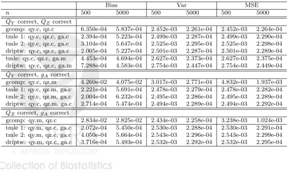
The results are detailed in tables 1 and 2. When the outcome expectation and the mediator density are correctly specified, the robust estimators TMLE and DR-IPTW provide little advantage over the g-computation estimator in terms of bias or efficiency. However, when either the outcome expectation or the mediator density are mis-specified, TMLE and DR-IPTW using a correct treatment mechanism provide substantial bias correction so that MSE is reducing at rate 1/n. The two robust estimators behave similarly. Moreover, as predicted by lemma 1, TMLE 2, which utilizes a mis-specified initial estimator of the mediated mean outcome difference, behaves as well as TMLE 1 when the treatment mechanism is correct.

Table 1: Simulation 1: Binary outcome, no positivity violations

Bias Var MSE

n 500 5000 500 5000 500 5000 ¯

QY correct,QZcorrect

gcomp: qy.c, qz.c 6.350e-04 5.837e-04 2.452e-03 2.261e-04 2.452e-03 2.264e-04 tmle 1: qy.c, qz.c, ga.c 2.394e-04 5.223e-04 2.499e-03 2.287e-04 2.499e-03 2.290e-04 tmle 2: qy.c, qz.c, ga.c 3.104e-04 5.647e-04 2.525e-03 2.295e-04 2.525e-03 2.298e-04 driptw: qy.c, qz.c, ga.c 2.005e-04 5.227e-04 2.501e-03 2.287e-04 2.501e-03 2.289e-04 tmle: qy.c, qz.c, ga.m 4.453e-04 4.694e-04 2.627e-03 2.373e-04 2.627e-03 2.375e-04 driptw: qy.c, qz.c, ga.m 7.288e-04 4.583e-04 2.754e-03 2.447e-04 2.754e-03 2.449e-04

¯

QY correct,gAcorrect

gcomp: qy.c, qz.m 4.260e-02 4.075e-02 3.017e-03 2.771e-04 4.832e-03 1.937e-03 tmle 1: qy.c, qz.m, ga.c 2.221e-04 5.691e-04 2.478e-03 2.279e-04 2.478e-03 2.282e-04 tmle 2: qy.c, qz.m, ga.c 2.004e-04 6.232e-04 2.495e-03 2.286e-04 2.495e-03 2.289e-04 driptw: qy.c, qz.m, ga.c 2.714e-04 5.474e-04 2.494e-03 2.289e-04 2.494e-03 2.292e-04

QZcorrect,gAcorrect

gcomp: qy.m, qz.c 2.834e-02 2.825e-02 2.434e-03 2.258e-04 3.238e-03 1.024e-03 tmle 1: qy.m, qz.c, ga.c 2.072e-04 5.450e-04 2.530e-03 2.288e-04 2.530e-03 2.291e-04 tmle 2: qy.m, qz.c, ga.c 4.050e-04 5.664e-04 2.543e-03 2.296e-04 2.543e-03 2.299e-04 driptw: qy.m, qz.c, ga.c 3.716e-04 5.493e-04 2.532e-03 2.292e-04 2.532e-03 2.295e-04

(20)

Table 2: Simulation 1: Continuous outcome, no positivity violations

Bias Var MSE

n 500 5000 500 5000 500 5000 ¯

¯

QZcorrect,gAcorrect

(21)

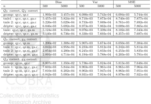
5.3.2 Simulation 2: larger effect of treatment on mediator

Under this simulation scheme, the parameters of interest are ψ0 = 0.12556476 for

the binary version, and ψ0 = 0.4183004 for the continuous version. The efficiency

bounds are var(D∗(P0)) = 3.721905 for the binary version, and var(D∗(P0)) =

17.53054 for the continuous version. Therefore, var(D∗(P0))/n ≈ 7.444e−03 and

7.444e−04 for n = 500 and 5000, respectively, in the case of the binary outcome, and var(D∗(P0))/n≈3.506e−02 and 3.506e−03 in the case of continuous Y.

In this simulation, the treatment has a moderately large effect on the mediator distribution. Compared to simulation 1, this simulation scheme has a larger ratio of

QZ(z|0, w)/QZ(z|1, w) for categories ofZ = 0,1 over a region of the sample space of

W (details are explained previously). We see that in this case all estimators behave as expected as in the previous simulation. When implemented using the correct treatment mechanism, they provide bias reduction over g-computation estimator in the cases when either the mediator density or the outcome model are mis-specified. When the outcome model and mediator density are both correct, then g-computation is consistent. In this case the TMLE and DR-IPTW are also consistent but less efficient. In all cases, TMLE and DR-IPTW behave similarly. We observe again that when the treatment mechanism is correct, TMLE 2, which utilizes a mis-specified initial estimator of the mediated mean outcome difference, behaves as well as TMLE 1.

Table 3: Simulation 2: Binary outcome, larger effect of treatment on mediator

Bias Var MSE

n 500 5000 500 5000 500 5000 ¯

gcomp: qy.c, qz.c 1.993e-03 3.457e-04 6.090e-03 5.743e-04 6.094e-03 5.744e-04 tmle1 : qy.c, qz.c, ga.c 5.457e-03 5.824e-04 8.710e-03 7.873e-04 8.740e-03 7.877e-04 tmle 2: qy.c, qz.c, ga.c 5.226e-03 5.029e-04 8.733e-03 7.889e-04 8.761e-03 7.892e-04 driptw: qy.c, qz.c, ga.c 6.046e-03 5.692e-04 8.973e-03 7.862e-04 9.009e-03 7.865e-04 tmle: qy.c, qz.c, ga.m 5.124e-03 6.550e-04 8.076e-03 7.339e-04 8.102e-03 7.343e-04 driptw: qy.c, qz.c, ga.m 5.140e-03 6.736e-04 8.330e-03 7.693e-04 8.357e-03 7.697e-04

¯

QZcorrect,gAcorrect

(22)

Table 4: Simulation 2: Continuous outcome, larger effect of treatment on mediator

Bias Var MSE

n 500 5000 500 5000 500 5000 ¯

¯

QZcorrect,gAcorrect

(23)

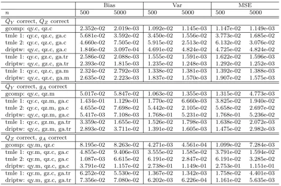
5.3.3 Simulation 3: Near positivity violation.

The parameters of interest are the same as in simulation 1: ψ0 = 0.2585079 for

the binary version, and ψ0 = 1.158052 for the continuous version. Probability of

treatment given covariate W is bounded between (0.0794,0.999994), with treatment probability >1.99 for W >1.5. Estimators using a truncated version of the correct treatment mechanism with an a-priori specified bound of (0.025, 0.975) were also considered (’ga.tr’).

In the presence of data sparsity, the robustness results of lemma 1 no longer apply when the treatment model values are extreme. We observe here that the MSE of TMLE and DR-IPTW in the case of mis-specification of outcome model or mediator density cease to reduce at a rate proportional to sample size. However, when both of the outcome model and mediator density are correct, TMLE and DR-IPTW with an incorrect treatment mechanism (either through truncation or incorrect modeling) yields MSE that are proportional to sample size. This last result is predicted by the robustness result (i) of lemma 1 and the fact that the mis-specified treatment models is bounded away from 1.

We observe also that in the case of near positivity violation, TMLE 2 is less favor-able than TMLE 1 across all cases. This may suggest that under data sparsity, the use of plug-in estimator for the mediated mean outcome difference is more beneficial than considerations such as the rate at which it is estimated. Interestingly, in table 5, which pertains to a binary outcome, we observe an increase in MSE (driven by the increase in variance) as one moves away from the use of substitution principle (with TMLE 1 being the one which uses substitution estimators in all its steps, TMLE 2 which does not use substitution estimator in the initial estimate of the mediated mean outcome difference but uses substitution in the final effect estimate, and DR-IPTW which does not use substitution at all). This may suggest that in the case of positivity violation, when strict bounds exist on the parameter, the degree at which each step of the estimation procedure respects the bounds affects the stability of the resulting estimate. Nonetheless, rigorous analysis is needed to provide more valid insights.

Unlike in previous two cases, we observe that TMLE and DR-IPTW behave dif-ferently in some cases. We first consider the version with binary outcome. Since the parameter is an average of probability differences, for a given dataset one would like the effect estimates to be bounded between −1 and 1. However, when using a correctly specified treatment mechanism, the DR-IPTW estimator exhibits estimates that are out of bound (of magnitude larger than 3 in some cases, and of magnitude 11 and 14 in one dataset). The bias, variance and mse of each estimator are detailed in table 5. When outcome model and mediator density are correct, the g-computation is still consistent despite the positivity violation. Nonetheless, the effect of data-sparsity on g-comp is apparent when comparing this g-comp estimator with its counterpart in the case of no positivity violation (table 1, line 1). On the other hand, under correct outcome model and mediator density, TMLE and DR-IPTW have poor variance when implemented with an untruncated correct treatment mechanism (’qy.c, qz.c, ga.c’). However, their performances are improved when implemented with a truncated or mis-specified treatment (’qy.c, qz.c, ga.tr’ and ’qy.c, qz.c, ga.m’). We also observe

(24)

that in the case of all models correct (’qy.c, qz.c, ga.c’), TMLE and DR-IPTW have a different bias-variance trade-off, with TMLE having smaller variance but larger bias, with respect to DR-IPTW (which has a larger variance but smaller bias). This differ-ence in relative bias and variance is also present in the case of mis-specified mediator density but correct outcome and treatment (’qy.c, qz.m, ga.c’): we observe that using the untruncated correct treatment, TMLE has larger bias and smaller variance than DR-IPTW; but when the truncated treatment mechanism is used, the two robust estimators behave similarly and provide bias reduction over the g-computation es-timator. When the outcome model is mis-specified, TMLE and DR-IPTW provide similar bias reduction over g-computation estimator. However, in this case TMLE has a smaller variance (than DR-IPTW) when the untruncated treatment mechanism is used, while the opposite is true when the truncated treatment mechanism is used. Consider now the case of continuous outcome (table 6). When the outcome model and mediator density are correct, the g-computation is consistent, though converging at a slower rate than its counterpart in the no-sparsity case (table 2, line 1) due to the larger variances. We also observe that when using an untruncated correct treatment mechanism (’qy.c, qz.c, ga.c’), the TMLE 1 has a larger bias but substantially smaller variance than the DR-IPTW in smaller sample size. This is likely due to some large effect estimates in DR-IPTW in the dataset with smaller sample size. The variance of DR-IPTW decreases substantially when sample size increases. On the other hand, when the treatment mechanism is truncated (’qy.c, gz.c, ga.tr’). DR-IPTW has now a smaller variance but larger bias than TMLE 1. When a mis-specified treatment mechanism is used, the two robust estimators behave similarly, but still have larger variance than the g-computation estimator. In the case of incorrect mediator density, when the untruncated treatment mechanism is used, we observe again that DR-IPTW has much smaller bias than TMLE 1, but substantially larger variance in finite sample (for the same reason mentioned above). This difference largely disappears when sam-ple size increases. But when the treatment is truncated, we observe again that TMLE has smaller bias but larger variance than DR-IPTW. In the case when the outcome model is incorrect: when the treatment is not truncated, TMLE 1 has larger bias and smaller variance than DR-IPTW, and that relation is reversed when truncation is applied.

(25)

Table 5: Simulation 3: Binary outcome, positivity violations inp(A|W)

Bias Var MSE

n 500 5000 500 5000 500 5000 ¯

gcomp: qy.c, qz.c 2.352e-02 2.019e-03 1.092e-02 1.145e-03 1.147e-02 1.149e-03 tmle 1: qy.c, qz.c, ga.c 5.681e-02 3.592e-02 3.450e-02 1.556e-02 3.773e-02 1.685e-02 tmle 2: qy.c, qz.c, ga.c 4.660e-02 7.505e-02 5.915e-02 2.513e-02 6.132e-02 3.076e-02 driptw: qy.c, qz.c, ga.c 1.846e-02 3.097e-04 4.691e-02 4.824e-02 4.725e-02 4.824e-02 tmle 1: qy.c, gz.c, ga.tr 2.586e-02 2.088e-03 1.555e-02 1.591e-03 1.622e-02 1.596e-03 driptw: qy.c, gz.c, ga.tr 2.393e-02 1.815e-03 1.235e-02 1.248e-03 1.292e-02 1.252e-03 tmle 1: qy.c, qz.c, ga.m 2.324e-02 2.792e-03 1.338e-02 1.381e-03 1.392e-02 1.388e-03 driptw: qy.c, qz.c, ga.m 2.635e-02 2.223e-03 1.837e-02 1.570e-03 1.907e-02 1.575e-03

¯

gcomp: qy.c, qz.m 5.017e-02 5.847e-02 1.063e-02 1.355e-03 1.315e-02 4.773e-03 tmle 1: qy.c, qz.m, ga.c 1.434e-01 1.129e-01 1.770e-02 6.660e-03 3.825e-02 1.940e-02 tmle 2: qy.c, qz.m, ga.c 4.655e-02 7.698e-02 5.442e-02 2.105e-02 5.658e-02 2.697e-02 driptw: qy.c, qz.m, ga.c 5.417e-03 7.108e-03 1.768e-01 5.231e-02 1.768e-01 5.236e-02 tmle 1: qy.c, gz.m, ga.tr 3.359e-02 1.655e-02 1.526e-02 1.798e-03 1.638e-02 2.072e-03 driptw: qy.c, gz.m, ga.tr 2.893e-02 3.711e-02 1.391e-02 1.605e-03 1.475e-02 2.982e-03

QZcorrect,gA correct

gcomp: qy.m, qz.c 8.195e-02 8.263e-02 4.271e-03 4.561e-04 1.099e-02 7.284e-03 tmle 1: qy.m, qz.c, ga.c 4.855e-02 9.406e-03 3.555e-02 1.585e-02 3.791e-02 1.594e-02 tmle 2: qy.m, qz.c, ga.c 1.087e-03 6.615e-02 6.191e-02 2.847e-02 6.191e-02 3.285e-02 driptw: qy.m, qz.c, ga.c 3.791e-02 1.157e-02 2.738e-01 1.149e-01 2.753e-01 1.151e-01 tmle 1: qy.m, gz.c, ga.tr 6.252e-02 5.530e-02 1.367e-02 1.342e-03 1.758e-02 4.401e-03 driptw: qy.m, gz.c, ga.tr 7.356e-02 7.080e-02 6.202e-03 6.226e-04 1.161e-02 5.635e-03

Table 6: Simulation 3: Continuous outcome, positivity violations in p(A|W)

Bias Var MSE

n 500 5000 500 5000 500 5000 ¯

gcomp: qy.c, qz.c 2.390e-03 3.603e-03 7.999e-02 8.030e-03 8.000e-02 8.043e-03 tmle 1: qy.c, qz.c, ga.c 6.235e-02 4.228e-02 7.509e-01 4.091e-01 7.548e-01 4.109e-01 tmle 2: qy.c, qz.c, ga.c 2.556e-01 4.214e-01 1.080e+00 6.355e-01 1.145e+00 8.130e-01 driptw: qy.c, qz.c, ga.c 1.847e-02 2.185e-02 1.836e+00 2.474e-01 1.836e+00 2.479e-01 tmle 1: qy.c, gz.c, ga.tr 2.895e-03 1.652e-03 1.227e-01 1.087e-02 1.227e-01 1.087e-02 driptw: qy.c, gz.c, ga.tr 2.733e-03 2.608e-03 8.762e-02 8.473e-03 8.763e-02 8.479e-03 tmle 1: qy.c, qz.c, ga.m 3.104e-04 4.806e-03 1.231e-01 1.209e-02 1.231e-01 1.212e-02 driptw: qy.c, qz.c, ga.m 6.349e-03 4.447e-03 1.497e-01 1.228e-02 1.497e-01 1.230e-02

¯

QY correct,gA correct

gcomp: qy.c, qz.m 2.927e-01 2.996e-01 8.383e-02 8.112e-03 1.695e-01 9.787e-02 tmle 1: qy.c, qz.m, ga.c 5.792e-01 4.894e-01 2.332e-01 1.429e-01 5.687e-01 3.824e-01 tmle 2: qy.c, qz.m, ga.c 2.114e-01 4.413e-01 9.927e-01 5.920e-01 1.037e+00 7.867e-01 driptw: qy.c, qz.m, ga.c 4.033e-02 6.585e-02 8.779e+00 1.899e-01 8.781e+00 1.943e-01 tmle 1: qy.c, gz.m, ga.tr 1.077e-01 8.515e-02 1.030e-01 1.046e-02 1.147e-01 1.771e-02 driptw: qy.c, gz.m, ga.tr 1.795e-01 1.873e-01 9.681e-02 9.235e-03 1.290e-01 4.433e-02

QZcorrect,gAcorrect

gcomp: qy.m, qz.c 1.553e-01 1.616e-01 2.087e-02 2.142e-03 4.499e-02 2.825e-02 tmle 1: qy.m, qz.c, ga.c 2.451e-02 2.284e-01 7.689e-01 4.513e-01 7.695e-01 5.035e-01 tmle 2: qy.m, qz.c, ga.c 7.633e-02 2.932e-01 1.051e+00 6.325e-01 1.057e+00 7.185e-01 driptw: qy.m, qz.c, ga.c 4.949e-02 9.666e-03 8.180e-01 7.365e-01 8.205e-01 7.366e-01 tmle 1: qy.m, gz.c, ga.tr 1.017e-01 1.108e-01 8.538e-02 6.351e-03 9.573e-02 1.862e-02 driptw: qy.m, gz.c, ga.tr 1.323e-01 1.361e-01 3.437e-02 3.049e-03 5.189e-02 2.157e-02

(26)

6 Summary

Using the framework of van der Laan and Rubin (2006), we have proposed a semi-parametric efficient, multiply robust substitution estimator for the natural direct effect of a binary exposure in a nonparametric model. The estimation procedure con-sists of targetedly modifying the conditional outcome expectation and the mediated mean outcome difference, in that order, and then obtaining the effect estimate as the marginal mean of the targeted mediated mean outcome difference. This estimator is asymptotically unbiased if either one of the following holds: i) the conditional out-come expectation given exposure, mediator, and confounders, and the mediated mean outcome difference are consistently estimated; (ii) the exposure mechanism given con-founders, and the conditional outcome expectation are consistently estimated; or (iii) the exposure mechanism given confounders, and the conditional mediator density ra-tio are consistently estimated. If all three condira-tions hold, then the effect estimate is asymptotically efficient.

In applications, the components that are difficult to estimate are often times the outcome model or the mediator density. Case (iii) implies in particular, that one may still obtain unbiased effect estimates without correct estimation of either of these components. More specifically, if the conditional distribution of treatment given confounders, and the conditional distribution of treatment given confounders and mediator are correct, then the targeted estimator will be asymptotically unbiased. Case (i) implies that if one can only consistently estimate the outcome model, but not the mediator density or treatment mechanism, it is still possible to obtain unbiased estimates if one has available a consistent initial estimator for the mediated mean outcome difference itself (e.g. a data-adaptive estimator which regresses the predicted outcome difference on the confounders, among control observations).

We have also described general conditions for the estimator to be asymptotically linear. More specifically, (a) estimators of each component must converge to their respective limits at a reasonable speed; (b) at most one component may be inconsis-tently estimated, in which case the consistent estimators of the remaining components must meet stricter asymptotic linearity conditions. These conditions provide a guide for situations where influence curve based variance estimates are realistic.

Estimators which make use of the efficient score are robust, but are generally sen-sitive to practical positivity violations. We refer to Petersen et al. (2010) for methods of diagnosing and responding to violations of the positivity assumption. The sub-stitution principle and the logistic working submodels in the targeted estimation procedure aims to provide more stable estimates in such situations. However, identi-fication of the parameter depends ultimately on the information available in the given finite sample. A way to improve finite sample robustness is the Collaborative TMLE framework of van der Laan and Gruber (2010), where, instead of estimating the true treatment mechanism, for a given initial estimator of theQcomponent one estimates a conditional distribution of the treatment, conditioned only on confounders which explain the residual bias of the estimator ofQ. We aim to investigate applications of Collaborative TMLE to the effect mediation problem.

(27)

References

R.M. Baron and D.A. Kenny. The moderator-mediator variable distinction in so-cial psychological research: Conceptual, strategic, and statistical considerations.

Journal of Penalty and Social Psychology, 51(6):1173–1182, 1986.

S. Gruber and M.J. van der Laan. A targeted maximum likelihood estimator of a causal effect on a bounded continuous outcome. The International Journal of Biostatistics, 6, 2010.

D.M. Hafeman and T.J. VanderWeele. Alternative assumptions for the identification of direct and indirect effects. Epidemiology, 2010.

P. Holland. Statistics and causal inference. Journal of the American Statistical As-sociation, 81:945–960, 1986.

K. Imai, L. Keel, and T. Yamamoto. Identication, inference and sensitivity analysis for causal mediation effects. Statistical Science, 25(1):51–71, 2010.

B. Jo, E. Stuart, and D. MacKinnon. The use of propensity scores in mediation analysis. Multivariabe behavior research, 46:425–452, 2011.

J. Kang and J. Schafer. Demystifying double robustness: A comparison of alternative strategies for estimating a population mean from incomplete data (with discussion).

Statistical Science, 22:523–39, 2007.

J.S. Kaufman, R.F. Maclehose, and S. Kaufman. A further critique of the analytic strategy of adjusting for covariates to identify biologic mediation. Epidemiologic Perspectives & Innovations, page 1:4, 2004.

M. Kosorok. Introduction to Empirical Processes and Semiparametric Inference. Springer, New York, 2008.

J. Pearl. Direct and indirect effects. In M. Kaufmann, editor, Proceedings of the Seventeenth Conference on Uncertainty in Artificial Intelligence, pages 411–420, 2000.

J. Pearl. Causality: Models, Reasoning and Inference. Cambridge University Press, New York, 2nd edition, 2009.

J. Pearl. The mediation formula: A guide to the assessment of causal pathways in nonlinear models. In C. Berzuini, P. Dawid, and L. Bernardinelli, editors,Causality: Statistical Perspectives and Applications. 2011.

M. Petersen, K. Porter, S.Gruber, Y. Wang, and M.J. van der Laan. Diagnos-ing and respondDiagnos-ing to violations in the positivity assumption. Technical report 269, Division of Biostatistics, University of California, Berkeley, 2010. URL

http://www.bepress.com/ucbbiostat/paper269.

(28)

J.M. Robins. Marginal structural models versus structural nested models as tools for causal inference. In Statistical models in epidemiology: the environment and clinical trials, pages 95–134. Springer-Verlag, 1999.

J.M. Robins. Semantics of causal dag models and the identification of direct and indirect effects. In N. Hjort P. Green and S. Richardson, editors,Highly Structured Stochastic Systems, pages 70–81. Oxford University Press, Oxford, 2003.

J.M. Robins and S. Greenland. Identifiability and exchangeability for direct and indirect effects. Epidemiology, 3(0):143–155, 1992.

J.M. Robins and A. Rotnitzky. Comment on the Bickel and Kwon article, “Inference for semiparametric models: Some questions and an answer”. Statistica Sinica, 11 (4):920–936, 2001.

P.R. Rosenbaum and Donald B. Rubin. The central role of the propensity score in observational studies for causal effects. Biometrika, 70:41–55, 1983.

D.B. Rubin. Bayesian inference for causal effects: the role of randomization. Annals of Statistics, 6:34–58, 1978.

E.J. Tchetgen Tchetgen and I. Shpitser. Semiparametric theory for causal mediation analysis: efficiency bounds, multiple robustness, and sensitivity analysis. Technical report 130, Biostatistics, Harvard University, June 2011.

A.A. Tsiatis. Semiparametric Theory and Missing Data. Springer, New York, 2006. M.J. van der Laan and S. Gruber. Collaborative double robust penalized targeted

maximum likelihood estimation.The International Journal of Biostatistics, 6, 2010. M.J. van der Laan and M. Petersen. Estimation of direct and indirect causal effects in longitudinal studies. Technical report 155, Division of Biostatistics, University of California, Berkeley, August 2004.

M.J. van der Laan and M.L. Petersen. Direct effect models.The International Journal of Biostatistics, 4(1), 2008.

M.J. van der Laan and J.M. Robins. Unified methods for censored longitudinal data and causality. Springer, New York, 2003.

M.J. van der Laan and S. Rose.Targeted Learning: Causal Inference for Observational and Experimental Data. Springer Series in Statistics. Springer, first edition, 2011. M.J. van der Laan and D.B. Rubin. Targeted maximum likelihood learning. The

International Journal of Biostatistics, 2(1), 2006.

A.W. van der Vaart. Asymptotic Statistics. Cambridge University Press, 1998. T.J. VanderWeele. Marginal structural models for the estimation of direct and indirect

effects. Epidemiology, 20:18–26, 2009.