A Dissertation by
SOUTIR BANDYOPADHYAY
Submitted to the Office of Graduate Studies of Texas A&M University
in partial fulfillment of the requirements for the degree of DOCTOR OF PHILOSOPHY
August 2010
A Dissertation by
SOUTIR BANDYOPADHYAY
Submitted to the Office of Graduate Studies of Texas A&M University
in partial fulfillment of the requirements for the degree of DOCTOR OF PHILOSOPHY
Approved by:
Chair of Committee, Soumendra N. Lahiri Committee Members, Raymond J. Carroll
Michael Sherman Gerald R. North Head of Department, Simon J. Sheather
August 2010 Major Subject: Statistics
ABSTRACT
On Parametric and Nonparametric Methods for Dependent Data. (August 2010) Soutir Bandyopadhyay, B.Sc., St. Xavier’s College;
M.Stat., Indian Statistical Institute
Chair of Advisory Committee: Dr. Soumendra N. Lahiri
In recent years, there has been a surge of research interest in the analysis of time series and spatial data. While on one hand more and more sophisticated models are being developed, on the other hand the resulting theory and estimation process has become more and more involved. This dissertation addresses the development of statistical inference procedures for data exhibiting dependencies of varied form and structure.
In the first work, we consider estimation of the mean squared prediction error (MSPE) of the best linear predictor of (possibly) nonlinear functions of finitely many future observations in a stationary time series. We develop a resampling methodology for estimating the MSPE when the unknown parameters in the best linear predictor are estimated. Further, we propose a bias corrected MSPE estimator based on the bootstrap and establish its second order accuracy. Finite sample properties of the method are investigated through a simulation study.
The next work considers nonparametric inference on spatial data. In this work the asymptotic distribution of the Discrete Fourier Transformation (DFT) of spa-tial data under pure and mixed increasing domain spaspa-tial asymptotic structures are studied under both deterministic and stochastic spatial sampling designs. The de-terministic design is specified by a scaled version of the integer lattice in IRd while the data-sites under the stochastic spatial design are generated by a sequence of in-dependent random vectors, with a possibly nonuniform density. A detailed account of the asymptotic joint distribution of the DFTs of the spatial data is given which,
among other things, highlights the effects of the geometry of the sampling region and the spatial sampling density on the limit distribution. Further, it is shown that in both deterministic and stochastic design cases, for “asymptotically distant” frequen-cies, the DFTs are asymptotically independent, but this property may be destroyed if the frequencies are “asymptotically close”. Some important implications of the main results are also given.
ACKNOWLEDGMENTS
I would like to thank my advisor, Professor Soumendra N. Lahiri for his guidance, help, encouragement and support throughout my days as a graduate student. The completion of my dissertation would have been impossible without his kind help and guidance.
I would also like to thank the members of my committee, Prof. Raymond J. Carroll, Prof. Michael Sherman and Prof. Gerald R. North, for finding time to serve and for their guidance and help.
I am also grateful to the Department of Statistics at Texas A&M University for providing me an excellent learning environment and for the financial assistance and support throughout my stay at TAMU. I would also like to thank Arnab Maity, a former graduate student of Texas A&M statistics department. I have spent many hours debating fine points and cooperatively solving problems with him. We learned many things together through cooperation and disagreement.
I am grateful to my teachers in Department of Statistics at St. Xavier’s College and Indian Statistical Institute. I would like to thank my uncle, Prof. Tathagata Bandyopadhyay, who inspired me to take up a research career in statistics. My friends, who supported, helped and encouraged me through all the good and bad times deserve my thanks.
Last but not the least, my parents and my wife, Rajeswari Banerji deserve the greatest thanks for supporting me and for being my source of strength and happiness.
TABLE OF CONTENTS
Page
ABSTRACT . . . iii
DEDICATION . . . v
ACKNOWLEDGMENTS . . . vi
TABLE OF CONTENTS . . . vii
LIST OF TABLES . . . x
LIST OF FIGURES . . . xi
CHAPTER I INTRODUCTION. . . 1
II RESAMPLING-BASED BIAS-CORRECTED TIME SERIES PREDICTION. . . 3
II.1. Introduction . . . 3
II.2. Bootstrap estimation of the MSPE . . . 7
II.2.1. Preliminaries . . . 7
II.2.2. Ordinary bootstrap estimator of the MSPE . . . 8
II.2.3. Limitations of the ordinary bootstrap estimator 11 II.3. Second order accurate estimation of the MSPE . . . 12
II.3.1. The tilting method . . . 12
II.3.2. Theoretical properties . . . 14
II.4. Practical implementation based on the bootstrap . . . 17
II.5. Simulation study . . . 20
II.6. Proofs . . . 22
II.6.1. Auxiliary lemmas . . . 24
CHAPTER Page III ASYMPTOTIC PROPERTIES OF DISCRETE FOURIER
TRANSFORMS FOR SPATIAL DATA . . . 36
III.1. Introduction . . . 36
III.2. Theoretical framework . . . 41
III.2.1. Sampling region . . . 41
III.2.2. Sampling design for regularly-spaced data-sites . 42 III.2.3. Stochastic sampling design - irregularly spaced case . . . 43
III.2.4. Regularity conditions on the random field . . . . 44
III.3. Results in the regularly-spaced case . . . 45
III.3.1. Results under PID . . . 45
III.3.1.1. Definition of the DFTs . . . 45
III.3.1.2. Asymptotic distribution at nonzero fre-quencies . . . 47
III.3.1.3. Asymptotic distribution for the zero limiting frequency . . . 51
III.3.1.4. Results for mean-corrected DFTs . . . 55
III.3.2. Results under the MID case . . . 56
III.4. Results under the stochastic design . . . 58
III.4.1. Definition of the DFT and some preliminaries . . 58
III.4.2. Asymptotic distribution at nonzero frequencies . 60 III.4.3. Asymptotic distribution for the zero limiting frequency . . . 63
III.4.3.1. Results for mean-corrected DFTs . . . 65
III.5. Some implications of the main results . . . 67
III.6. Proofs of the results from Section III.3 . . . 68
III.6.1. Preliminaries . . . 68
III.6.2. Proof of Theorem III.3.1 . . . 73
III.6.3. Proof of Theorem III.3.2 . . . 74
III.6.4. Proof of Theorem III.3.3 . . . 76
III.6.5. Proof of Theorem III.3.4 . . . 77
III.6.6. Proof of Theorem III.3.5 . . . 78
III.7. Proofs of the results from Section III.4 . . . 78
III.7.1. Preliminaries . . . 78
III.7.2. Proof of Theorem III.4.1 . . . 79
III.7.3. Proof of Theorem III.4.2 . . . 80
CHAPTER Page
III.7.5. Proof of Theorem III.4.4 . . . 82
IV CONCLUSION . . . 84
REFERENCES . . . 87
LIST OF TABLES
TABLE Page
1. Bias and root mean squared error (RMSE) for the estimators (with and without bootstrap based bias correction) of the mean squared prediction errors for models in (II.5.1)-(II.5.2) for sample size(n) = 50, 120 and 500, number of replications(N) = 500 and
LIST OF FIGURES
FIGURE Page
1 Boxplots of RMSE values of the estimators (with bias-correction (b.c.) and without bias correction (n.b.c.)) of the mean squared prediction errors for n=50, 120 and 500 under the three models
CHAPTER I
INTRODUCTION
We consider analysis of dependent data in which interest focuses on developing dif-ferent inference procedures for the population-level quantities. In the first work a parametric approach has been adopted for the estimation of the mean squared pre-diction error of the best linear predictor of (possibly) nonlinear functions of finitely many future observations in a stationary time series.
A random field or a spatial process is a generalization of a stochastic process such that the underlying parameter need no longer be a simple real, but can instead be a multidimensional vector space or even a manifold. Due to advances in science and technology, high-throughput spatial data from neuroscience and environmental (among other) applications are being generated at a rapid pace. This has created an urgent need for methodology and tools for analyzing regularly as well as irregularly spaced spatial data. In biological applications, advances in microscope automation are yielding an abundance of data on spatial patterns of neuronal activation. Using digital imaging modalities, it is now possible to collect replicated patterns over large areas of the brain. Another important application in epidemiology is the geographical disease surveillance using scan statistics. Spatial scan statistics are widely used for count data to detect geographical disease clusters of high or low incidence, mortal-ity or prevalence and to evaluate their statistical significance. In the environmental and climate sciences, measurements are often recorded at different locations on many variables. Formulating correct statistical models that make sense of all the many com-This dissertation follows the style of the Journal of the Royal Statistical Society.
plex relationships and multivariate dependencies that are in the data, investigating the properties of these models and developing inferential procedures have provided major challenges for statisticians, probabilists and others working in this field. In the next work we concentrate on developing a nonparametric inference method for regularly as well as irregularly spaced spatial data.
In recent years, there has been a surge of research interest in the analysis of spa-tial data using the frequency domain approach. At a heuristic level, the popularity of the frequency domain approach lies in the fact that for equi-spaced time series data, the discrete Fourier transform (DFT) of the observations are asymptotically independent. As a result, it allows one to avoid accounting for the dependence in the data explicitly. However, validity of the asymptotic independence of the DFTs for spatial data remains largely unexplored. In contrast to the time series case where observations are usually taken at a regular interval of time and asymptotics is driven by the unidirectional flow of time, for random processes observed over space, several different types of spatial sampling designs and spatial asymptotic structures are rele-vant for practical applications. For example, image data are equi-spaced in the plane, but locations of the drilling-sites for mineral ores in a mine are usually irregularly spaced. Thus, the type of asymptotics that are appropriate in these applications are inherently different. We investigated in detail the asymptotic properties of the DFT for equi-spaced as well as irregularly spaced spatial data under different types of spatial asymptotic structures.
CHAPTER II
RESAMPLING-BASED BIAS-CORRECTED TIME SERIES PREDICTION
II.1. Introduction
Let {Xt}∞t=−∞ be a second order stationary time series with auto-covariance function γ(·) and spectral density f(·). Suppose that a finite stretch, X1, . . . , Xn of the series is observed. In many applications, it is important to predict an unobserved future valueXn+k in the time series or more generally, a suitable functional of a set of future values Xn+1, . . . , Xn+k:
Ψ =ψ(Xn+1, . . . , Xn+k)
where ψ : IRk → IR is a known function and k ∈ IN. Here and in the following, IN and ZZ respectively denote the set of all positive integers and the set of all integers. A popular predictor of Ψ is given by the best linear predictor (BLP) ˜Ψn =α1X1 +
. . .+αnXn, where (λ1, . . . , λn) = argmina1,...,anE Ψ−[a1X1+. . .+anXn] 2 . (II.1.1)
The co-efficients λ1, . . . , λn can be found by standard optimization arguments from calculus; See (II.2.1), Section II.2 below for an explicit expression for λ1, . . . , λn. Typically, λ1, . . . , λn in ˜Ψn depend on the auto-covariance function γ(·) and, for a nonlinear ψ(·), on other population parameters of the {Xt}-process and hence, are typically unknown in practice. Here we restrict attention to parametric time series models and highlight the dependence of the BLP on the underlying parameters by writing
˜
where θ ∈ IRp (p ∈ IN) is the vector of unknown parameters of the {Xt}-process. Since ˜Ψ(θ) depends on unknown θ, it is not usable in practice. A common approach is to plug-in an estimator ˆθn of the unknown parameter θ in ˜Ψn(θ), yielding the estimated best linear predictor (EBLP):
ˆ
Ψn= ˜Ψn(ˆθn). (II.1.2)
An important problem in time series analysis is to accurately estimate the mean squared prediction error (MSPE) of the EBLP:
M(θ)≡E ˆ Ψn−Ψn(θ) 2 . (II.1.3)
Like the BLP ˜Ψn(θ), the MSPE also depends on the unknown parameter vector θ. Note that the functionM(θ)≡Mn(θ) can be represented as
M(θ) = EΨ˜n(θ)−Ψ 2 + 2Eh{Ψˆn−Ψ˜n(θ)}{Ψ˜n(θ)−Ψ} i +EΨˆn−Ψ˜n(θ) 2 ≡ M1(θ) +M2(θ) +M3(θ), say. (II.1.4)
The first term M1(θ) ≡ M1n(θ) is the MSPE of the ideal predictor ˜Ψn(θ), the third termM3(θ)≡M3n(θ) is the estimation error due to the substitution of ˆθn in place of θin ˜Ψn(·), and the second one is a cross-product term. Thus, the MSPE of the EBLP depends on the MSPE of the ideal predictor as well as on the particular estimator ˆθn used for estimating the unknown parameter vector θ. Except for some very specific cases, analytic expressions for the functionsMi(θ),i= 1,2,3 (particularly,M2(θ) and
M3(θ)) are not available in the literature, making the estimation of the MSPE M(θ)
difficult by the traditional plug-in approach. In this chapter, we propose a bootstrap based method to derive an estimator of the MSPEM(θ). The key advantage of the bootstrap methodology is that it produces an estimator of the MSPE of the EBLP
for any given estimator ˆθn of θ, without requiring any analytical computation of the functionsM2(θ) andM3(θ) which critically depend on the choice of ˆθn. We show that under fairly mild regularity conditions on the {Xt}-process and on the estimators ˆθn, the bootstrap MSPE estimator is consistent.
Next we consider higher order accuracy of the resulting bootstrap estimator. Typically, of the three terms Mi(θ), i= 1,2,3, the first one is O(1), while the second and the third terms are typically O(n−1), as the sample size n goes to infinity. As
a result, usual consistency of the “ordinary” bootstrap MSPE estimator of M(θ) is not adequate in many applications where the sample size only moderately large and the effects of theO(n−1) terms can not be ignored. Indeed, it can be shown that the bootstrap MSPE estimator has a bias of the orderO(n−1), which is of the same order
as the orders of the terms Mi(θ), i = 2,3. Thus, the “ordinary” bootstrap MSPE estimator masks the contributions coming from parameter estimation in ˜Ψn(θ) to the overall MSPE of ˆΨn. What is needed is an estimator of the MSPE of ˆΨn that has a bias of order o(n−1) and still retains the standard order of convergence; Following
Prasad and Rao (1990), we call such estimators of the MSPE M(θ) second order correct. A common way to construct a second order correct MSPE estimator is to use the explicit bias correction to a plug-in estimator of M(θ). However, this is impractical and undesirable in our situation mainly because of two reasons, namely, (i) explicit analytical expressions for Mi(θ), i = 1,2,3 are very rarely available in the literature (only in some simple toy models) as these are very difficult to derive in reasonable generality, and (ii) the explicit bias correction leads to a negative estimator of the MSPE with a positive probability. An important contribution of this work is to develop a new method for constructing a second order correct MSPE estimator that is non negative with probability one. The key idea is to “tilt” the estimator ˆθn suitably so that it balances out the bias of the “ordinary” bootstrap MSPE estimator
to the order O(n−1). The tilting factor used here is based on certain iterations of the bootstrap step and on a simple formula to combine them. As a result, the computation of the proposed second order correct MSPE estimator is very much feasible with today’s computing power, and the methodology works any choice of the estimator ˆθn satisfying the mild regularity conditions of the main result. Most importantly, the proposed method does not require any analytical derivation on the part of the user.
The rest of the chapter is organized as follows. We conclude this section with a brief literature review. In Section II.2, we describe the “ordinary” bootstrap estimator of the MSPE and prove its consistency. The tilted version of the MSPE estimator and its theoretical properties are stated in Section II.3. In Section II.4, we develop some bootstrap based approximations for different functions appearing in the tilted MSPE estimator, for which exact analytical expressions are either unavailable or intractable. In Section II.5, we report the results from a simulation study on finite sample properties of the proposed tilted MSPE estimator. Proofs of the main results are presented in Section II.6.
The literature on time series prediction is huge and is well documented in the case where the target variable Ψ =Xn+kfor somek; See Brockwell and Davis (1991), Priestley (1981). For standard stationary time series models, like the autoregressive (AR) processes and autoregressive and moving average (ARMA) processes, explicit expressions for M1(θ) is known (cf. Brockwell and Davis (1991)), although
expres-sions for M2(θ) and M3(θ) are not common. The masking-effect of the naive plug-in
approach on MSPE estimation was pointed out by Prasad and Rao (1990), who also introduced the concept of second order bias corrected MSPE estimators, in the context of small area estimation. For a detailed account of the literature on issues and solutions in the small area estimation problem until 2003, see Rao (2003). In
the time series context, Ansley and Kohn (1986) and Quenneville and Singh (2000) proposed different MSPE estimators based on analytical considerations for the state-space model. More recently, Pfeffermann and Tiller (2005) proposed a bootstrap based method for MSPE estimation of the best linear unbiased predictor (BLUP), also for the state-space model under a Gaussian assumption. The second order cor-rect MSPE estimation methodology presented here is different from the earlier work on the problem in the time series literature; It is based on the approach developed by Lahiri and Maiti (2003) and Lahiri et al. (2007) in the context of small area estimation.
II.2. Bootstrap estimation of the MSPE II.2.1. Preliminaries
In this section, we formalize the basic framework for bootstrap estimation of the MSPE. As in Section II.1, let{Xt}∞t=−∞be a second order stationary time series with an absolutely summable auto-covariance function γ(·) and spectral density f(·), and for a known function ψ :IRk →IR let
Ψ =ψ(Xn+1, . . . , Xn+k)
is to be predicted using the observations X1, . . . , Xn. For the ease of exposition and
as it is customary in the time series literature (see Chapter 5, Brockwell and Davis (1991)), for the rest of this chapter, we shall suppose that the variables Xt’s and Ψ have mean zero. Thus, the focus of the work is on the prediction of the random part; The deterministic mean part, if any, can be estimated by any of the standard methods, such as (quasi-)maximum likelihood, method of moments, etc., which in turn, can be used for mean correction. Under the zero-mean assumption, it is easy to derive an explicit expression for the BLP ˜Ψn using standard arguments. Thus, by
differentiating the expression on the right side of (II.1.1), it is easy to show that the vector λn ≡(λ1, . . . , λn)0 of co-efficients in ˜Ψn are given by
λn≡λn(θ) = Γ−n1γn, (II.2.1) where Γn≡Γn(θ) is the n×n matrix with (i, j)th element cov(Xi, Xj), 1≤i, j ≤n, and where γn ≡ γn(θ) = (cov(Ψ, X1), . . . ,cov(Ψ, Xn))0. Here and in the following, we drop θ from population quantities, except when it is important to highlight the dependence on θ and similarly, often drop n from subscript, for simplicity of exposi-tion. Note that by the Pythagorus theorem, the MSPE of the ideal predictor ˜Ψn is given by
M1n(θ) = var(Ψ)−γ0nΓ −1
n γn.
However, exact expressions for the second and the third terms in (II.1.4) are not easy to write down and both of these terms depend on the particular estimator ˆθn is used. In the next section, we describe a resampling method for estimating all three components of the MSPE of the EBLP ˆΨn.
II.2.2. Ordinary bootstrap estimator of the MSPE
Let ˜θn be an estimator of θ based on X1, . . . , Xn. We shall use ˜θn to produce the bootstrap estimator of the MSPE M(θ). In principle, one may take ˜θn = ˆθn, but a different choice of ˆθn may be more appropriate in a specific application. The main steps in the ordinary bootstrap estimation procedure are as follows:
A. Generate a bootstrap sample X1∗, . . . , Xn∗ under the θ = ˜θn. Let θn∗ denote the bootstrap version of ˆθn obtained by replacingX1, . . . , Xn by X1∗, . . . , X
∗ n. B. Compute ˆΨ∗n = ˜Ψn(θn∗) by replacing θ inλ(θ) (see (II.2.1)) by θ∗n.
C. The bootstrap estimator of M(θ) is given by [ mspeorn =E∗ ˆ Ψ∗n−Ψ∗n 2 , (II.2.2)
where Ψ∗n = ψ(X1∗, . . . , Xn∗) is the bootstrap version of the predictand Ψ and where E∗ denotes conditional expectation given X1, . . . , Xn.
In practice, evaluation of the conditional expectation is done by the Monte-Carlo method. For this, steps A-C are repeated a large number (say, B) of times and the resulting bootstrap replicates are combined. Specifically, for each b = 1, . . . , B, one generates thebth resampleX1∗b, . . . , Xn∗b under theθ= ˜θn (independently of the other replicates) and then computes θ∗bn, ˆΨ∗bn = ˜Ψn(θn∗b) and Ψ
∗b n = ψ(X ∗b 1 , . . . , X ∗b n ) based onX1∗b, . . . , Xn∗b as in steps A-C. The Monte-Carlo approximation tomspe[orn is given by [ mspeor:mcn =B−1 B X b=1 ˆ Ψ∗bn −Ψ∗bn 2 . (II.2.3)
The following result shows that the ordinary bootstrap estimator of the MSPE is consistent under mild conditions on the underlying time series {Xt}∞
t=−∞ and on the estimator sequences {θˆn}n≥1 and {θ˜n}n≥1.
Theorem II.2.1. Let θ0 denote the true value of the parameter θ and let Θ0 ={θ ∈
Θ :kθ−θ0k ≤δ0} for some δ0 ∈(0,∞). Suppose that θn˜ −θ0 =op(1) as n→ ∞ and that the following conditions hold:
(A.1) There exists δ∈(0,1] such that (i) sup{EθΨ2 :θ∈Θ
0}< δ−1, and
(ii) δ < fθ(ω)≤δ−1 for all ω∈(−π, π) and θ ∈Θ0.
(A.2) (i) For eachj ≤0, gj(θ)is continuous at θ =θ0 and |gj(θ)| ≤aj for all θ∈Θ0, where P0
j=−∞aj <∞.
(A.3) sup{M3n(θ) :θ∈Θ0} →0 as n → ∞. Then
[
mspeorn −Mn(θ0)→p 0 as n → ∞. (II.2.4) Conditions (A.1)-(A.3) are local uniformity conditions on various second order population quantities (moments) related to the time series{Xi}∞i=−∞, and essentially requires continuity of the parametric model at θ = θ0. Condition (A.1)(i) requires
that the second moment of the predictand Ψ be bounded in a neighborhood of the true parameter value θ0, which would hold ifEθ0Ψ2 <∞ and EθΨ2, as a function ofθ, is continuous atθ=θ0. Condition (A.1)(ii) is a crucial condition that is used all through
the chapter. It is used to obtain some bounds on the spectral norm of the matrix Γn(θ) and its inverse. This condition is satisfied when {Xi}∞i=−∞ is an ARMA(p, q)-process where all roots of the corresponding characteristic polynomial lie outside the unit circle (see Brockwell and Davis (1991)). Next consider (A.2). Continuity ofgj(·) at θ = θ0 is tied down to the continuity of the model parametrization at θ = θ0.
The local uniform summability of gj(θ)’s can be replaced by requiring finiteness and continuity of the absolute sum P
j≤0|gj(θ)| on Θ0, in which case aj corresponds to |gj(θ1)| for all j ≤ 0, for a common θ1 ∈ Θ0. Alternatively, it is guaranteed if some
standard mixing and moment conditions hold. More specifically, suppose that the process {Xi}∞i=−∞ is strongly mixing with the mixing co-efficient
α(n;θ)≡sup{|Pθ(A∩B)−Pθ(A)Pθ(B)|:A ∈ F−∞j ,Fj−∞+n, j ∈ZZ}, (II.2.5) where Fb
a = σhXt : t ∈ [a, b]∩ZZi, −∞ ≤ a ≤ b ≤ ∞. Let α0(n) = supθ∈Θ0α(n;θ), n ≥ 1. If E|Ψ|2+δ < ∞ and P∞
n=1α0(n) δ
2+δ < ∞, then (A.2)(i) holds. Condition
(A.2)(ii) requires a form of continuity of the parametric model at θ = θ0, and is
above. It can be further ascertained if the functionEθX0Xj is continuous at θ =θ0
for each j ≥0, and for some δ >0,E|X1|2+δ <∞and
P∞
n=1α0(n) δ
2+δ <∞. Finally,
consider (A.3). As pointed out before, the function M3n(θ) quantifies the effect of
replacing the unknown true value of the parameter by the estimator ˆθn in the (ideal) BLP, and hence, it critically depends on the properties of the estimator sequence {θˆn}n≥1. Typically, for a sequence of consistent estimators {θˆn}n≥1, M3n(θ0) → 0.
Condition (A.3) requires the convergence to be uniform in a neighborhood of θ0. We
impose the condition directly on M3n(·) to keep the statement of Theorem II.2.1 simple, which only claims consistency of the ordinary bootstrap estimator of the MSPE. A set of sufficient conditions for (A.3) is given in Section II.3, where a more precise bound (namely, O(n−1)) on the order of M
3n(·) is obtained.
II.2.3. Limitations of the ordinary bootstrap estimator
It is easy to see that the ordinary bootstrap estimator of the true MSPE Mn(θ0)
is equivalent to the plug-in estimator Mn(˜θn), and has the added advantage that it does not require an explicit expression for the three components Min(θ0), i = 1,2,3
(see (II.1.4)). However, as explained earlier, of the three terms in (II.1.4), only the leading term M1n(θ0) = O(1) while the terms Min(θ0), i = 2,3 are typically of the
order O(n−1). Therefore, Theorem II.2.1 asserts consistency of bootstrap estimator
[
mspeorn for M1n(θ0), the MSPE of the ideal predictor ˜Ψn, only and fails to capture the effects of estimating the unknown θ0 by ˆθn, leading to the termsMin(θ0), i= 2,3
in the overall MSPE Mn(θ0) of the EBLP ˆΨn. For a better approximation, effects
of the terms Min(θ0), i = 2,3 must be taken into account. In the next section, we
describe an implicit bias-correction method based on the bootstrap that achieves this goal.
II.3. Second order accurate estimation of the MSPE II.3.1. The tilting method
We first describe the tilting method in our MSPE estimation problem. The basic idea behind the tilting method is to replace the original estimator ˆθnwith a suitably tilted
(or perturbed) estimator of θ that annihilates the bias contribution of ˆθn to M1n(·), up to the second order accuracy. Suppose that
p
X
j=1
|M1(jn)(θ0)|> 0, (II.3.1)
for some0 >0, where for a smooth functionf :IRp →IR,f(i),f(i,j)andf(i,j,k)denote
the first, the second and the third order partial derivatives with respect to the i-th co-ordinate, the (i, j)-th co-ordinates, and the (i, j, k)-th co-ordinates, respectively, i, j, k= 1,· · ·, p. Condition (II.3.1) says that M1(in)(θ0)6= 0 for some i. For notational
simplicity, we suppose that M1(1)n(θ0) 6= 0. Next let βn ≡ βn(θ) and Σn = Σn(θ) respectively denote the the bias and variance of ˆθn. We shall also suppose that some consistent estimators ˆβnand ˆΣnofβnand Σn, respectively, are available. For example, under mild conditions on ˆθn and {Xt}, such estimators can be generated using the bootstrap method (see Lahiri (2003a)). Then the preliminary tilted estimatorof θ is defined as ˆθn+rn, where rn is given by,
rn =− " p X i=1 M1(in)(ˆθn) ˆβn,i+ 1 2 p X i=1 p X j=1 M1(ni,j)(ˆθn) ˆΣn(i, j) # n M1(1)n(ˆθn) o−1 e1, (II.3.2)
where, ˆβn,i and ˆΣn(i, j) denote the ith component of ˆβn and (i, j)th component of ˆ
Σn, respectively, and where the vector e` ∈ IRp has one in the `th position and zeros elsewhere, 1 ≤ ` ≤ p. Thus, the preliminary tilted estimator is obtained from the initial estimator ˆθn by adding a correction factor to the first component of ˆ
θn only. Note that if, instead of M
(1)
1n(·), a different partial derivative M
(i)
nonzero, then we would define the preliminary tilted estimator by replacing the factor n M1(1)n(ˆθn) o−1 e1 in (II.3.2) with n M1(ni)(ˆθn) o−1 ei.
To make the MSPE estimator well-defined and to ensure its consistency, we need to modify the preliminary tilted estimator ˆθn+rn. The modifications are needed either if ˆθn+rn falls outside Θ, in which case Mn(ˆθn+rn) is not well defined, or ifM
(1) 1i (ˆθn) becomes too small, in which case, it scales up the variability of the correction factor
rn. Under appropriate regularity conditions, the probability of getting a preliminary estimator ˆθn+rn outside Θ or that of getting a value ofM
(1)
1n(ˆθn) below the threshold (1 + logn)−2 tends to zero rapidly as n → ∞. As a consequence, the perturbed estimator ˇθn coincides with the preliminary perturbed estimator ˆθn +rn with high probability.
The tilted estimator of the MSPE is now defined as
[
mspen =Mn(ˇθn) (II.3.3)
where ˇθn is the tilted estimatorof θ, defined by ˇ θn= ˆ θn+rn if ˆθn+rn∈Θ and |M (1) 1n(ˆθn)|−1 ≤(1 + logn)2 ˆ θn otherwise. (II.3.4)
Although an explicit expression for the functionMn(·) is typically unknown, it is not difficult to see that the tilted estimator mspe[n is equivalently given by (II.2.2) with ˜
θn= ˇθn; The latter can be computed using the algorithm given in Section II.2.2. In the next section, we state the regularity conditions and show that the tilted estimator of the MSPE in (II.3.3) achieves second order bias accuracy.
II.3.2. Theoretical properties
As before, let θ0 denote the true value of the parameter θ and let Θ0 = {θ ∈ Θ :
kθ−θ0k ≤δ0}denote a open neighborhood ofθ0. LetPθ andEθdenote the probability
and expectation underθ. For notational simplicity, we setPθ0 =P and Eθ0 =E. For j ∈ZZ, define
gj(θ) = Eθ[ψ(X1, . . . , Xk)Xj], θ∈Θ.
Note that gj(θ) is the covariance between Xn+j and Ψ = ψ(Xn+1, . . . , Xn+k) under θ, which decreases to zero as j → −∞ under suitable weak dependence and moment conditions on{Xi}∞i=−∞. Let ∆λn(θ) be thep×n matrix, with ith column given by the p×1 vector of partial derivatives of theith component of λn(θ) =γn(θ)Γn(θ)−1. Define µ2n(θ) ≡ nEθ [ˆθn−θ]0∆λn(θ)Xn{λn(θ)Xn−Ψ} µ3n(θ) ≡ Eθ n1/2[ˆθn−θ]0∆λn(θ)Xn 2 ,
which respectively give approximations to the functions M2n(θ) andM3n(θ), upto an error of order o(n−1). We shall use the following regularity conditions to prove the
results.
(C.1) Suppose that there exists aδ ∈(0,∞) such that lim inf
n→∞ M
(1)
1n(θ0)≥δ.
(C.2) Suppose that there exists κ, c0 ∈(0,∞) such that for allθ ∈Θ:
(i) EθΨ2 < c0,
(ii) Eθ|X1|4+κ < c0,
(iii) lim supn→∞Eθ
n√
nkθˆn−θk
o8
(C.3) Suppose that gj(θ) and fθ are twice differentiable on Θ, and that there exist a constant c1 ∈(0,∞) and a sequence {an}n≥1 ⊂(0,∞) with
P∞
n−1aj <∞ such that for all k, l∈ {1, . . . , p},
(i) max{gj(θ),|g (k) j (θ)|,|g (k,l) j (θ)|}< aj for all θ ∈Θ, (ii) max{kfθk∞,kfθ−1k∞,kf (k) θ k∞,kf (k,l)
θ k∞} < c1 for all |a| ≤ 2 and for all
θ ∈Θ, and
(iii) kfθ(k,l)−fθ0(k,l)k ≤c1kθ−θ0kδ, for all θ ∈Θ0 for some δ >0.
(C.4) Suppose that there exists ac2 ∈(0,∞) such that sup{|µkn(θ)|:θ∈Θ}< c2 for
all n≥c2, and µkn(·) is equi-continuous at θ=θ0, k = 2,3.
(C.5) Suppose thatβn(θ) =n−1β0(θ) +o(n−1) and Σn(θ) =n−1Σ0+o(n−1) uniformly
in θ ∈Θ and ∆0 ≡sup{kβ0k+kΣ0(θ)k:θ∈Θ}<∞.
Condition (C.1) is a specialized version of (II.3.1) for the given formula for the correction factor rn, which says that the function M1n(·) has a non-zero derivative along one of the directions i ∈ {1, . . . , p} at the true value θ0, and is typically
sat-isfied in most applications. See the discussion following (II.3.1) for implications and alternative versions of this. Condition (C.2)(i) is needed to makeM1n(·) well-defined while Conditions (C.2)(ii) and (iii) are used to establish exact orders of the func-tions Mkn(·) fork = 2,3 (see Lemma II.6.2 below). Condition (C.3) is a smoothness condition on the spectral density of the process {Xt} and on the cross-covariances gj(θ) = covθ(Ψ, Xj), which would hold if the underlying model-parametrization is suitably smooth. The same comment applies to Condition (C.4), which requires boundedness and equi-continuity of the approximating functions µkn, k = 2,3. Fi-nally, Condition (C.5) is a condition on the bias and the variance of the estimator sequence {θˆn}n≥1. We have decided to state Conditions (C.4) and (C.5) in terms of
the original sequence{θˆn}n≥1 to allow for generality. For a specific choice of ˆθn, these conditions have to be checked directly. To indicate the type of arguments one would need to verify (suitable variants) of these conditions, consider the class of estimator sequences{θˆn}n≥1 that admit a representation of the form:
ˆ θn−θ= β0(θ) n +n −1 n X i=1 ξi +Rn (II.3.5)
for some function β0(·) : Θ → IRp, zero mean random vectors ξi ∈ σhXii, i ≥ 1
and a remainder term Rn. Suppose that there exist constants δ, c3 ∈ (0,∞) and
a sequence {dn}n≥1 satisfying dn = o(n−1/2) such that kβ(θ)k < c3, Eθkξik8 < c3,
Eθkd−n1Rnk8 < c3 and P
∞ n=1n
3α(n;θ)8+δδ < c
3 for allθ ∈Θ. Then, it is easy to check
that Conditions (C.2)(iii) and (C.5) hold. Under (II.3.5), it can be shown that a variant of Condition (C.4) holds where the factor n1/2(ˆθ
n−θ) in the functions µkn are replaced by the leading to terms from (II.3.5). For example, for k = 3, it can be shown that under (C.3),
supn µ3n(θ)−µ˜3n(θ) :θ ∈Θ o =o(1). (II.3.6) where ˜ µ3n(θ)≡Eθ h n−1/2 n X i=1 ξi i0 ∆λn(θ)Xn 2 .
As a result, one can use ˜µ3n(θ) in place of µ3n(θ) as an approximation to M3n(θ) to establish Theorem II.3.1 (retracing the steps given in Section II.6). Note that the equi-continuity of ˜µ3n(θ) atθ=θ0 can now be proved under a continuity condition on
the individual lag-covariance functionsEθ[X1, ξ1][Xk+1, ξk+1]0, k ≥ 0 (as functions of
θ) as in Condition (A.2) and the discussion following the statement of Theorem II.2.1. We give a proof of (II.3.6) in Section II.6. A similar treatment is possible also for the termµ2n(θ). Hence, it follows that for an estimator sequence {θn}n≥ˆ 1 satisfying
(II.3.5), Conditions (C.2) - (C.5) hold under mild moment conditions on the variables Xt’s and ξt’s and under mild weak dependence conditions on the underlying process. With this, we are now ready to state the main result of this section.
Theorem II.3.1. Suppose that Conditions (C.1) - (C.5) hold. Then
Emspe[n−Mn(θ0) = o(n−1) (II.3.7) var(mspe[n−Mn(θ0) = O(n−1). (II.3.8)
Theorem II.3.1 shows that under suitable regularity conditions, the tilted MSPE estimator attains second order bias accuracy. Further, the variance of the tilted esti-mator continues to be of the same order as the untiled (naive) MSPE estiesti-mator, and is guaranteed to be non-negative. Thus, the tilted MSPE estimator may be preferred over the ordinary MSPE estimator that fails to capture the effects of parameter es-timation in the EBLP on the overall MSPE. In the next section, we describe some important issues related to the implementation of the titling method in practice.
II.4. Practical implementation based on the bootstrap
Note that the tilting method described above involves computing the functionsMin(·), i= 1,2,3, and its first and second order partial derivatives, for which explicit expres-sions are not always available. In this section, we develop bootstrap based approxima-tions to these quantities, so that the tilted MSPE estimator can be used in practice, without any analytical derivations. To that end, first we define a bootstrap-based approximation to the function M1n(·) at a given value θ = θ1 (which may depend
on the data). The steps are similar to those used for generating the Monte-carlo approximation tomspe[orn in (II.2.3). Specifically, for b= 1,· · ·, B,
B. Compute ˜Ψ∗bn and Ψ∗b by replacingX1, . . . , XnwithX1∗b,· · ·, Xn∗b+k. The Monte-carlo approximation to M1n(θ1) is given by
M1∗n(θ1) = B−1
B
X
b=1
( ˜Ψ∗bn −Ψ∗b)2. (II.4.1)
Next we construct estimates of the partial derivatives of the functionM1n(·) for computing the correction factor rn. To motivate the construction, first consider a smooth functiong :IR→IR. Then, for any x∈IR, using Taylor series expansion,
g(x+)−g(x−) = 2g0(x) +o(),
as→0, whereg0(x) denotes the derivative ofg(x) atx. Hence we can use the scaled difference (2)−1{g(x+)−g(x−)} as an approximation to g0(x) for small values
of >0. Relying on this fact, we can now define suitable bootstrap approximations to the first order partial derivatives of M1n(·) at ˆθn. Let {an}n≥1 be a sequence of
positive real numbers converging to zero. Then, withM1∗n as in (II.4.1), we define the bootstrap approximation to the first order partial derivatives as,
M1∗n(j)(ˆθn) = (2an)−1
h
M1∗n(ˆθn+anej)−M1∗n(ˆθn−anej)
i
, (II.4.2)
j = 1,· · ·, p. Similarly, we can define the bootstrap approximations to the second order partial derivatives as:
M1∗n(j,j)(ˆθn) = a−n2 h M1∗n(ˆθn+anej) +M1∗n(ˆθn−anej)−2M1∗n(ˆθn) i , 1≤j ≤p, M1∗n(i,j)(ˆθn) = 2a−n2 hn M1∗n(ˆθn+anei,j) +M1∗n(ˆθn−anei,j)−2M1∗n(ˆθn) o −a2nnM1∗n(i,i)(ˆθn) +M ∗(j,j) 1n (ˆθn) oi , 1≤i6=j ≤p. (II.4.3) where,ei,j =ei+ej.
Then, we have the following result on the accuracy of the bootstrap estimates of the partial derivatives:
Proposition II.4.1. Suppose Conditions (C.2) and (C.3) hold. Then,
E∗ M ∗(j) 1n (ˆθn)−M (j) 1n(ˆθn) 2
=O(B−1a−n2+a2n) almost surely for all 1≤j ≤p and
E∗ M ∗(i,j) 1n (ˆθn)−M (i,j) 1n (ˆθn) 2
=O(B−1a−n4+a2n) almost surely for all 1≤i, j ≤p.
Thus, by choosingansmall and then choosing the number of bootstrap replicates B suitably large, we can generate accurate approximations to the first and second order partial derivatives of the function M1n(·). Analytical derivations of the partial derivatives, therefore, can be completely bypassed by using the bootstrap (and hence, necessary computing resources).
Next, we define the bootstrap estimators of the bias and variance of ˆθn by, βn∗ = 1 B B X b=1 ˆ θn∗b−θˆn, Σ∗n = ( 1 B B X b=1 ˆ θ∗bn(ˆθ∗bn)0 ) − 1 B B X b=1 ˆ θn∗b ! 1 B B X b=1 ˆ θ∗bn !0 (II.4.4) respectively, where ˆθ∗bn denote thebth bootstrap replicate of ˆθn, obtained by replacing X1, . . . , Xn with X1∗b,· · ·, Xn∗b and {(X1∗b,· · ·, Xn∗b) : b = 1, . . . , B} are independent bootstrap replicates underθ = ˆθn.
Proposition II.4.2. Suppose Conditions (C.2), (C.3) and (C.5) hold. Then,
E∗ β ∗ n−βn 2
and E∗ Σ ∗ n−Σn 2
=O(B−1n−2) +o(n−2) almost surely.
Combining (II.4.2), (II.4.3) and (II.4.4) , we now define the bootstrap based correction factor as r∗n =− " p X i=1 M1∗n(i)(ˆθn)βn,i∗ + 1 2 p X i=1 p X j=1 {M1∗n(i,j)(ˆθn)}{Σ∗n(i, j)} # (II.4.5) ×n e1 M1∗n(1)(ˆθn) o,
where βn,i∗ and Σ∗n(i, j) respectively denote the ith component of βn∗ and the (i, j)th element of Σ∗n, 1 ≤ i, j ≤ p. The bootstrap-based bias-corrected MSPE estimate is given by
[
mspe∗n=mspe[or:mcn (ˇθ ∗
n) (II.4.6)
where mspe[or:mcn (ˇθn∗) is defined by (II.2.3) with ˜θn = ˇθ∗n, and ˇθ ∗ n is defined by replacing rn and M (1) 1n(ˆθn) in (II.3.4) byr∗n and M ∗(1) 1n (ˆθn), respectively.
In view of Theorem II.3.1 and Propositions 4.1 and 4.2,mspe[∗n gives an accurate approximation to the bias-corrected estimator of the MSPE that can be evaluated without any analytical work, provided Conditions (C.1)-(C.5) hold. However, finite sample performance of the MSPE estimator depends on the choice of different factors, such as an, B, etc. In the next section, we explore these issues further through a simulation study.
II.5. Simulation study
For the simulation study, we consider one-step-ahead best linear prediction, i.e., we take the predictand Ψ to be Xn+1. We shall consider the the following time series
Model 1: In the linear autoregressive model of order 2, AR(2),
Xt =φ1Xt−1+φ2Xt−2+t, (II.5.1) fort ∈Z, where {t} are independent and identically distributed N(0, σ2). Values of φ1, φ2 are chosen to be (0.2,0.5) and the value of σ2 is 4.
Model 2: In the linear autoregressive moving-average model of order (1,1), ARMA (1,1),
Xt=φ1Xt−1+t+ψ1t−1, (II.5.2)
for t ∈ Z, where {t} are independent and identically distributed N(0, σ2). Here we take the parameter values to beφ1 = 0.2, ψ1 = 0.5 and we takeσ2 = 4.
In this simulation study, we will perturb the estimator in the direction of σ2.
In implementing the method, we use B = 1000 bootstrap samples to estimate the bias, variances and for all other approximations. All simulation results are based on N = 500 replications. The simulations are done for n = 50,120 and 500. Table 1 reports the empirical measures of bias and root mean squared error (RMSE) for both bias-corrected and not bias-corrected estimators mspe[∗n and mspe[
or:mc
n of MSPE
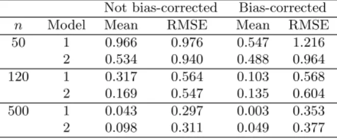
for three different values ofn. The bias and mean squared error (MSE) are estimated empirically by taking the average over the replicates of the bias and MSE for each dataset. From Table 1 we can see that the bias correction method gives us significantly better results for different values ofnunder the models (II.5.1) and (II.5.2). However, it is worth mentioning that due to the bias correction, the RMSE’s of the bias-corrected estimators are seemed to be slightly higher than the not bias-bias-corrected
Table 1. Bias and root mean squared error (RMSE) for the estimators (with and without bootstrap based bias
correction) of the mean squared prediction errors for models in (II.5.1)-(II.5.2) for sample size(n) =
50, 120 and 500, number of replications(N) = 500 and number of bootstrap samples(N0) = 1000. Not bias-corrected Bias-corrected
n Model Mean RMSE Mean RMSE 50 1 0.966 0.976 0.547 1.216 2 0.534 0.940 0.488 0.964 120 1 0.317 0.564 0.103 0.568 2 0.169 0.547 0.135 0.604 500 1 0.043 0.297 0.003 0.353 2 0.098 0.311 0.049 0.377
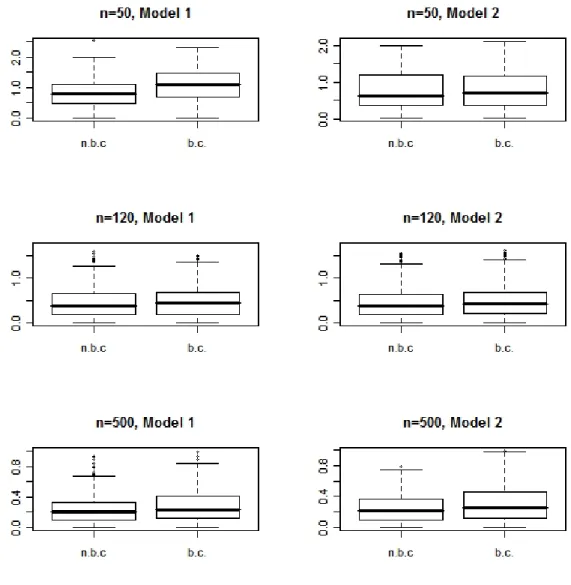
estimators. This is expected, as the randomness in the various approximation steps in the construction of the bias-corrected estimators adds to its total variability. Boxplots for RMSE’s of the two estimators of MSPE overN = 500 simulations under different models are presented in Figure 1. The boxplots also support the conclusions obtained from Table 1. In these boxplots we can see that due to the bias correction the RMSE’s of the tilted estimators seem to be higher than the unperturbed estimators.
II.6. Proofs
For a l×l matrix A, let kAk = sup{kAxk : x ∈ IRl,kxk = 1} denote the spectral norm, where 1 ≤ l ≤ ∞ and where k · k denotes the `2 norm on IR2. Let ZZ+ =
{0,1,2, . . .}. For a= (a1, . . . , ap)0 ∈ ZZ p +, let |a| =|a1|+. . .+|ap|, a! = Qp i=1ai! and Da=D1a1. . . Dap
p , where Dj denotes the partial derivative w.r.t. thejth co-ordinate, 1 ≤ j ≤ p. Let C, C(·) denote generic constants with values in (0,∞) that depend on their arguments, if any, but not on n. Unless otherwise specified, limits in order symbols are taken by letting n→ ∞.
Fig. 1Boxplots of RMSE values of the estimators (with bias-correction (b.c.) and without bias correction
(n.b.c.)) of the mean squared prediction errors for n=50, 120 and 500 under the three models as in
II.6.1. Auxiliary lemmas
Lemma II.6.1. Suppose that gj(θ) and fθ are twice differentiable on Θ, and that
there exists a constantC0 >0 such that (i) P j≤0|D ag j(θ)|2 < C0 for all θ∈Θ, (ii) kfθk∞+kfθ−1k∞+kD af
θk∞< C0 for all |a| ≤2 and for all θ ∈Θ, and (iii) kDaf
θ−Dafθ0k ≤C0kθ−θ0kδ, for all θ∈Θ0 for some δ >0. Then, there exists a constant C1 ∈ (0,∞) such that |M
(j)
1n(θ)|+|M
(i,j)
1n (θ)| < C1 for all θ ∈ Θ and for all n ≥ C1, where 1 ≤ i, j ≤ p. Further,
P
1≤i,j≤p|M
(i,j) 1n (θ0)−
M1(i,jn )(θ)| ≤C1kθ0−θkδ for all θ∈Θ0 and for all n ≥C1. ProofIt is easy to check that for θ1, θ2 ∈Θ,
γn(θ1)0Γn(θ1)−1γn(θ1)−γn(θ2)0Γn(θ2)−1γn(θ2) = γn(θ1)−γn(θ2) 0 Γn(θ1)−1γn(θ1) +γn(θ2)Γn(θ1)−1 γn(θ1)−γn(θ2) +γn(θ2)0Γn(θ2)−1 h Γn(θ2)−Γn(θ1) i Γn(θ1)−1γn(θ2),
which, in view of conditions (i), (ii) and (II.6.4), readily implies that DjM1n(θ) = [Djγn(θ)]0Γn(θ)−1γn(θ) +γn(θ)0Γn(θ)−1[Djγn(θ)]
−γn(θ)0Γn(θ)−1[DjΓn(θ)]Γn(θ)−1γn(θ).
Next using similar arguments for the second derivation (which is now given by nine terms), one can complete the proof of the lemma. We omit the details.
Lemma II.6.2. Suppose that there exists κ, C ∈(0,∞) such that (i) Eθ|X1|4+κ < C,
(iii) lim supn→∞kγn(θ)k< C, and
(iv) kf−1
θ k∞< C
for allθ ∈Θ. Then, supθ∈Θh
M3n(θ)−n −1µ 3n(θ) + M2n(θ)−n −1µ 2n(θ) i =o(n−1). Proof Note that on the set An≡ {kθ−θˆnk ≤},
[λn(ˆθn)−λ(θ)]Xn = [ˆθn−θ]0[∆λn(θ)]Xn+
X
|a|=2
[ˆθn−θ]aDaλ(θ1)Xn/a! whereθ1 is a point in An. Hence,
M3n(θ)−Eθ [ˆθn−θ]0∆λn(θ)Xn 2
≤ C(p) sup{|Daλ(t)||kt−θk ≤,|a|= 2}Eθk˙ θnˆ −θk4kXnk211(An) +Eθ
[|λn(ˆθn)Xn|+|λn(θ)Xn|]·11(kθˆn−θk ≥δ)
2
≡ I1+I2 +I3, say.
First consider I2. Let Xn,i = (X1,i, . . . , Xn,i)0, i = 1,2 where Xj,1 =Xj11(|Xj| ≤ cn) and Xj,2 =Xj−Xj,1, 1 ≤j ≤n, where cn=n1/2−κ/16. By (iii) and (iv), there exists c0 ∈ (0,∞) such that kλn(θ)k2 = γn(θ)0Γ(θ)−2γn(θ) < c20 for all θ ∈ Θ, for n large.
Hence, we have, for any >0, Eθ [λn(ˆθn)Xn]·11(kθˆn−θk ≥) 2 ≤ 2Eθ [λn(ˆθn)0Xn,1]·11(Acn) 2 + 2Eθ λn(ˆθn)0Xn,2 2 ≤ 2c20h Eθ Xn i=1 [Xi,21−EθX12,1]11(Acn) +nEθX 2 1,1Pθ(Acn) i + 2c20EθkXn,2k2 ≤ Cc20 h n ∞ X i=1 |cov(X12,1, Xi,21)|1/2Pθ(Acn) 1/2 +nEθX12Pθ(Acn) +EθX1211(|X1|> cn) i
≤ Cc20n−1−
for some=(κ)>0. By similar arguments, I3 ≤Cc20n−1−. Also,
I1 ≤ CEθkθˆn−θk4kbf Xnk211(An) ≤ Eθ kθˆn−θk4 hXn i=1 (Xi,21−EθXi,21) +nEθX12,1+ n X i=1 (X22,1i11(An) ≤ CEθ kθnˆ −θk811(An) 1/2 n ∞ X i=1 |cov(X12,1, Xi,21)|1/2 +CnEθX12Eθkθˆn−θk411(An) +Cn(EθX24,1)
1/2(E
θkθˆn−θk811(An))1/2 ≤ Cc20n−1−
for some=(κ)>0.
The proof of the second relation follows by repeating the same arguments, and there-fore, it is omitted.
Lemma II.6.3. For j ≥1 and 1 ≤k ≤4, let ξkj be a σhXji-measurable zero-mean
random variable such that for some δ, c1 ∈ (0,∞), Eθ|ξkj|4+δ < c1 for all j, k and P∞
n=1n
3α(n;θ)4+δδ < c
1 for all θ ∈ Θ. Let {ekjn : 1 ≤ j ≤ n}n≥1 ⊂ IR be such that Pn
j=1e2kjn = O(1) for 1≤ k ≤ 4. Then there exists a constant C1 (depending on c1, but not on θ) such that
lim sup n→∞ n Eθ hXn i=1 ξ1i Y3 k=2 Xn i=1 ekjnξki i +Eθ hY4 k=1 Xn i=1 ekjnξki io < C1 for all θ∈Θ.
Proof We shall give a proof of the bound on the second term only; the proof of the bound on the first term is similar (and somewhat simpler). Clearly, for any 1≤k, l≤4, Eθ Xn i=1 ekinξki Xn j=1 eljnξlj
≤ n−1 X
|m|=0
X
{(i,j):i−j=m,1≤i,j≤n}
ekineljnEθξkiξlj ≤ n−1 X |m|=0 X
{(i,j):i−j=m,1≤i,j≤n}
|ekineljn|Eθ|ξki|2+δ 1 2+δ Eθ|ξlj|2+δ 1 2+δ α(|m|;θ)2+δδ ≤ n−1 X |m|=0 hXn i=1 e2kini 1/2hXn i=1 e2lini 1/2 C(c1, δ)α(|m|;θ) δ 2+δ ≤C(c1, δ) n−1 X m=0 α(m;θ)2+δδ.
Let K4(V1, V2, V3, V4) denote the fourth order (mixed) cumulant of a set of random
variablesV1, V2, V3, V4 under θ, defined by
K4(V1, V2, V3, V4;θ) = ∂ ∂v1 ∂ ∂v2 ∂ ∂v3 ∂ ∂v4 Eθexp(√−1[v1V1+v2V2+v3V3+v4V4]) v1=...=v4=0.
Then, by using multi-linearity ofK4(·), it follows that
Eθ hY4 k=1 Xn i=1 ekjnξki i ≤ K4( n X i=1 e1jnξ1i, . . . , n X i=1 e4jnξ4i) + X I⊂{1,2,3,4},|I|=2 K2( n X i=1 ekjnξki, k ∈I)( n X i=1 ekjnξki, k ∈Ic) . Note that |K2( n X i=1 ekjnξ1i, k∈I)| ≤ Y k∈I h var Xn i=1 ekinξki i1/2 ≤ Y k∈I hXn i=1 e2kinEθ(ξki)2+ 2 n−1 X j=1 n−j X i=1 e2kin 1/2 Xn i=j+1 e2kin 1/2 |cov(ξki, ξk(i+j))| i1/2 = O(1) uniformly in θ ∈Θ.
Next writing ˇein = max{|ekin|:k = 1,2,3,4}, 1≤i≤n, and writing
P
b for the sum over alli1, . . . , i4 ∈ {1, . . . , n} with maximal gap b, 0≤b≤n−1, we have,
K4( n X i=1 e1jnξ1i, . . . , n X i=1 e4jnξ4i) ≤ C n−1 X b=0 X b 4 Y k=1 |ekikn||K4(ξ1i1, . . . , ξ4i4)| ≤ C n−1 X b=0 X b 4 Y k=1 |ekikn|c 4 4+δ 1 α(b;θ) δ 4+δ ≤ C(c1, δ) n−1 X b=0 hXn i=1 ˇ ein n X |ik−i|≤b,k=1,2,3 3 Y k=1 ˇ eikn oi α(b;θ)4+δδ ≤ C(c1, δ) n−1 X b=0 hXn i=1 ˇ ein 3 Y k=1 b1/2 X |ik−i|≤b ˇ e2i kn 1/2i α(b;θ)4+δδ ≤ C(c1, δ) n−1 X b=0 b3/2 hnXn i=1 ˇ e2in o1/2nXn i=1 3 Y k=1 X |ik−i|≤b ˇ e2ikn o1/2i α(b;θ)4+δδ ≤ C(c1, δ) n−1 X b=0 b3/2hn n X i=1 ˇ e2ino 1/2n b n X i=1 ˇ ein bmax{ˇe2in: 1≤i≤n}2}iα(b;θ)4+δδ ≤ C(c1, δ) hXn−1 b=0 b3α(b;θ)4+δδ i ×h ∞ X n=1 n3α(n;θ)4+δδ i ×hmax{ˇe2in: 1≤i≤n}2}i = O(1) uniformly in θ ∈Θ.
II.6.2. Proofs of the main results
Proof of Theorem II.2.1 It is enough to show that, |M1n(˜θn)−M1n(θ0)|+ 3 X i=2 |Min(˜θn)|+|Min(θ0)| =op(1). (II.6.1) Note that by (C.2) and the condition ˜θn
p →θ0, |M1n(˜θn)−M1n(θ0)|=op(1) if, γn(˜θn) 0 Γ−n1(˜θn)γn(˜θn)−γ(θ0) 0 Γ−n1(θ0)γn(θ0) = op(1). (II.6.2)
It is easy to check that the absolute value of the right side of (II.6.1) is bounded above by |γn(˜θn) 0 (Γn−1(˜θn)−Γn−1(θ0))γn(˜θn)| +2kγn(˜θn)−γn(θ0)kkΓ−n1(θ0)k kγn(˜θn)k+kγn(θ0)k ≡I1n+I2n, say. (II.6.3)
By using the standard isometric isomorphism between `2(ZZ) and L2(0,2π) through
the Fourier-Plancherel transform (see Bhatia (2003), Rudin (1987)), we have, kΓ−n1(θ)k ≤ Ckfθ−1k∞
kΓn(θ1)−Γn(θ2)k ≤ Ckfθ1 −fθ2k∞, for all θ1, θ1 ∈Θ, n ≥1. (II.6.4)
By (II.6.4) and conditions (C.2) and (C.3), I1n = |γn(˜θn)
0
Γ−n1(θ0)(Γn(˜θn)−Γn(θ0))Γ−n1(˜θn)γn(˜θn)| ≤ kγn(˜θn)k2kΓ−n1(θ0)kkΓn(˜θn)kkΓn(˜θn)−Γn(θ0)k
= op(1).
By similar arguments, on the set{kθ˜n−θ0k< }, (0< < δ),
I22n ≤ Ckγn(˜θn)−γn(θ0)k2 = C "M−1 X j=0 |gj(˜θn)−gj(θ0)|2 + n−1 X j=M |gj(˜θn)−gj(θ0)|2 # ≤ C "M−1 X j=0 sup kxk≤ |gj(θ0+x)−gj(θ0)|+ ∞ X j=M sup θ∈Θ0 |gj(θ)| #
Given any η > 0, there exist M ≥ 2, such that, P∞
j=M supθ∈Θ0|gj(θ)| < η
[3C]. Next,
givenM ≥1 and η >0, there exists ∈(0, δ) such that sup kxk≤ |gj(θ0+x)−gj(θ0)|< η 3M C, for all j = 0, . . . , M. Hence, P(I22n> η) ≤ P(kθ˜n−θ0k> ) +P(I22n> η,kθ˜n−θ0k< δ) ≤ P(kθ˜n−θ0k> ) + 0 for large n = o(1). By similar arguments, P(M3n(˜θn)> ) ≤ P(sup{M3n(θ) :θ∈Θ0}> ,θ˜n∈Θ0+P(˜θn 6∈Θ0) = o(1). Since M2n(θ)≤2 h M1n(θ)M3n(θ) i1/2
for all θ, the theorem is proved.
Proof of (II.3.6) Note that by Lemma II.6.3, sup{|µ˜3n(θ)|:θ∈Θ}=O(1). Hence, noting that sup{(EθkRnk8)1/8 :θ ∈Θ}=O(dn) = o(n−1/2), it is enough to show that
supn µ˜3n(θ)−Eθ h n−1/2β0(θ)+n−1/2 n X i=1 ξi i0 ∆λn(θ)Xn 2 :θ∈Θ o =o(1). (II.6.5) Now expanding the second term and applying the first part of Lemma II.6.3, one can conclude that the left side of (II.6.5) is in fact O(n−1). This completes the proof of (II.3.6).
Proof of Theorem II.3.1By (C.1), there existsC ∈(0,∞) such that sup{|M1(1)n(θ)|−1
:θ ∈Θ0, j, l= 1,· · ·, p;n ≥1}< C. Let ˆ Dn = p X j=1 M1(nj)(ˆθn) ˆβn,j+ p X j=1 p X l=1 w(j, l)M1(j,li )(ˆθn) ˆΣn(j, l)
˜ Dn = p X j=1 M1(ij)(θ0) ˆβn,j + p X j=1 p X l=1 w(j, l)M1(ij,l)(θ0) ˆΣn(j, l),
n ≥ 1, where w(j, l) = 1/2 for j 6= l and w(j, l) = 1 for j = l. Then by Taylor’s expansion, it follows that there exists a constant C ∈ (0,∞) such that on the set {θˆ∈Θ0}, ˆ Dn = ˜Dn+R1n, and rn=− ˜ Dn M1(1)n(θ0) e1+R2ne1 (II.6.6) where|R1n| ≤C n kβˆnk.kθˆn−θ0k+kθˆn−θ0kγkΣˆnk o and |R2n| ≤C n |Dˆn|.kθˆn−θ0k+ |R1n| o .
LetA1n≡ {θˆn∈Θ0} ∩ {θˆn+rn∈Θ}. Using similar arguments, on the set A1n, for all u∈[0,1], we have
p X j=1 p X l=1 w(j, l)M1(njl)(ˆθn+urn) [ˆθn+rn]−θ0 ej+el = p X j=1 p X l=1 w(j, l)M1(njl)(θ0) ˆ θn−θ0 ej+el +R3n(u)
where supu∈[0,1]|R3n(u)| ≤C
h
k(ˆθn+rn)−θ0k2+γ+k (ˆθn+rn)−θ0k · kθˆn−θ0k
+krnk2] for someC ∈(0,∞).
Next define the setA2n=A1n∩ {θˆn+rn∈Θ0}. Then, on A2n={θˆn,θˆn+rn ∈ Θ0}, by Taylor’s expansion, there exists a pointθ†n on the line joining ˆθn+rn and θ0
such that M1i(ˆθn+rn)−M1i(θ0) = p X j=1 M1(nj)(θ0) n [ˆθn+rn]−θ0 oej + p X j=1 p X l=1 w(j, l)M1(jli )(θ†n)n[ˆθn+rn]−θ0 oej+el = p X j=1 M1(nj)(θ0) ˆ θn−θ0 ej +M1(1)n(θ0) − ˜ Dn M1(1)n(θ0) +R2n ! + p X j=1 p X l=1 w(j, l)M1(njl)(θ0) n ˆ θn−θ0 oej+el +R†3n
= p X j=1 M1(nj)(θ0) ˆ θn−θ0 ej −βˆn,j + p X j=1 p X l=1 w(j, l)M1(ij,l)(θ0) ˆ θn−θ0 ej+el −Σˆn(j, l) +M1(1)n(θ0)R2n+R † 3n ≡ Q1n+M (1) 1n(θ0)R2n+R † 3n, say (II.6.7)
whereR†3n=R3n(u) with the u corresponding to θn†. Hence, on the set A3n ≡ {|M
(1) 1n(ˆθn)|−1 ≤(1 + logn)2}, M1n(ˇθn)−M1n(θ0) = [M1n(ˆθn+rn)−M1n(θ0)]11 n ˆ θn+rn ∈Θ o ∩A3n +[M1n(ˆθn)−M1n(θ0)]11 n ˆ θn+rn ∈/ Θ o ∪Ac3n = [M1n(ˆθn+rn)−M1n(θ0)] n 11(A2n) + 11(ˆθn+rn ∈Θ)−11(A2n) o 11(A3n) +[M1n(ˆθn)−M1n(θ0)]11 n ˆ θn+rn ∈/ Θ o ∪Ac3n ≡ hQ1n+M (1) 1n(θ0)R2n+R † 3n i 11(A2n∩A3n) +R4n, say ≡ Q1i+R5n,say, (II.6.8)
where|R5n| ≤ |R4n|+|R2n+R†3n|11(A2n) +|Q1n|11(Ac2n∩Ac3n) and |R4n| ≤ M1n(ˆθn+rn)−M(θ0) · 11(ˆθn+rn∈Θ)−11(A2n) 11(A3n) + M1n(ˆθn−M1n(θ0) 11({ ˆ θn+rn ∈/ Θ0} ∪Ac3n) ≡ R41n, say.
Note that by definition,
11(ˆθn+rn∈Θ)−11(A2n) ≤ 11(ˆθn+rn∈Θ)11(Ac2n) + 11(ˆθn+rn ∈/ Θ)11(A2n) ≤ {11(ˆθn ∈/ Θ0) + 11(ˆθn+rn∈Θ\Θ0)}+ 11(∅).
Hence, with Ac4n ≡ {θˆn+rn∈/ Θ0} ∩A3n, R41n ≤ M1n(ˆθn+rn)−M1n(ˆθn) 11(A3n){11(ˆθn ∈/ Θ0) + 11(ˆθn+rn∈Θ\Θ0)} +2 M1n(ˆθn)−M1n(θ0) n 11(ˆθn∈/ Θ0) + 11 {θˆn+rn ∈/Θ0} ∩A3n +11(Ac3n)o ≤ Ckrnk11(A3n) n 11(ˆθn ∈/ Θ0) + 11(ˆθn+rn∈Θ\Θ0) o +Ckθˆn−θ0k n 11(ˆθn∈/ Θ0) + 11(Ac4n) + 11(A c 3n) o ≤ C·(logn)2{kβˆnk+kΣˆnk}{11(ˆθn ∈/ Θ0) + 11(Ac4n)} +C· kθˆn−θ0k n 11(ˆθn∈/ Θ0) + 11(Ac4n) + 11(A c 3n) o . (II.6.9)
By condition, there existC ∈(0,∞) and1 ∈(0,02) such that
Ac4n ⊂ {kθˆn−θ0k> 0 2} ∪ {krnk> 0 2} ⊂ {kθnˆ −θ0k> 1} ∪ {(logn)2(kβnkˆ +kΣnk)ˆ > C} (II.6.10) and Ac
3n ⊂ {kθˆn−θ0k> 1} for all n ≥1. Hence, it follows that
R41n ≤ C·(logn)2{kβˆnk+kΣˆnk} h 11(kθˆn−θ0k> 1) +11 [logn]2(kβnkˆ +kΣnk)ˆ > C i +C· kθnˆ −θ0k h 11(kθnˆ −θ0k> 1) +11[logn]2(kβˆnk+kΣˆnk)> C i (II.6.11) for all n ≥ 1. Let Wn = (nkβˆnk+nkΣˆnk). Note that by uniform integrability of {(√nkθˆ−θk)2}m≥
1 and the fact that E |Wn |1+η=O(1),
E(R41n) ≤ Cn−1(logn)2hE |Wn|1+η 1+1η P(kθˆn−θ0k> 1 1+ηη +E | |Wn |1+η {n−1(logn)2}η i +Ch−11Ekθˆn−θ0k211(kθˆn−θ0k> 1)
+Ekθˆn−θ0k2 1/2n
P(n−1(logn)2|Wn|> C)
o12i
= o(n−1) as m → ∞. (II.6.12)
This proves the first part of Theorem II.3.1.
Next we consider the bound on the variance of the tilted MSPE estimator. Since sup{|Mkn(θ)|2 : θ ∈ Θ} = O(n−2) for k = 2,3, by Cauchy-Schwarz inequality, it is enough to show that
VarM1n(ˇθn) =O(n−1). (II.6.13) By Taylor’s expansion, M1n(ˇθn) = M1n(θ0) + p X j=1 M1(nj)(θ0)[ˇθn−θ0]ej+R6n
where |R6n| ≤ C(p)∆kθˇn−θ0k2 and ∆r = lim supn→∞sup{|M1αn(θ)| : θ ∈ Θ,|α| = r}, r = 1,2. Also, let A5n = {θˆn+rn ∈ Θ,|M (1) 1n(ˆθn)|−1 ≤ (1 + logn)2}. Thus, it follows that ER62n ≤ C(p,∆2)Ekθnˇ −θ0k4 = C(p,∆2) h Ekθˆn+rn−θ0k411(A5n) +Ekθˆn−θ0k411(Ac5n) i ≤ C(p,∆2)23 h Ekθˆn−θ0k4+Ekrnk411(A5n) i ≤ C(p,∆0,∆1,∆2) h Ekθˆn−θ0k4+ (1 = logn)8n−4 i = O(n−2). (II.6.14)
By similar arguments and Cauchy-Schwarz inequality, E h ˇ θn−θ0 iei+ej = Ehθˆn−θ0 iei+ej +OEkrnk211(A5n) + n Ekθˆn−θ0k2 o1/2n Ekrnk211(A5n) o1/2
Hence, it follows that Var Xp j=1 M1(nj)(θ0)[ˇθn−θ0]ej = p X i=1 p X j=1 M1(ni)(θ0)M1(jn)(θ0)cov [ˇθn−θ0]ei,[ˇθn−θ0]ej = p X i=1 p X j=1 M1(ni)(θ0)M (j) 1n(θ0)cov [ˇθn−θ0]ei,[ˇθn−θ0]ej = O(n−1). (II.6.15)
Hence, by (II.6.14), (II.6.15), and Cauchy-Schwarz inequality, (II.6.13) follows. This completes the proof of Theorem II.3.1.
Proof of Proposition II.4.1Forb= 1, . . . , B, let Υ∗b1j = ˜Ψ∗bn(ˆθn+anej)−Ψ∗bn(ˆθn+ anej) and let Υ∗b2j be defined by replacing ˆθn+anej by ˆθn−anej in Υ∗b1j, 1 ≤j ≤ p. Then, by Taylor’s expansion
E∗M ∗(j) 1n (ˆθn)−M1n(ˆθn) = (2an) −1hM 1n(ˆθn+anej)−M1n(ˆθn−anej) i −M1n(ˆθn) ≤ Cansup{M1n(θ) :θ ∈Θ}.
Next, by (conditional) independence of {Υ∗b
kj :b= 1, . . . , B}, k = 1,2, var∗([2Ban]−1 B X b=1 [Υ∗b1j−Υ∗b2j]) =O(a−n2B−1), k= 1,2.
This proves the first part of Proposition II.4.1. The proof of the second part is similar and hence, is omitted.
Proof of Proposition II.4.2Similar to the proof of Proposition II.4.1 and hence is omitted.
CHAPTER III
ASYMPTOTIC PROPERTIES OF DISCRETE FOURIER TRANSFORMS FOR SPATIAL DATA
III.1. Introduction
In recent years, there has been a surge of research interest in the analysis of spatial data using the frequency domain approach; see for example, Hall and Patil (1994), Im et al. (2007), Fuentes (2002, 2005, 2007), and the references therein. At a heuristic level, the popularity of the frequency domain approach lies in the fact that for equi-spacedtime series data, the discrete Fourier transform (DFT) of the observations are asymptotically independent (see Kawata (1966,1969), Fuller (1976) and Brockwell and Davis (1991), Lahiri (2003c)). As a result, it allows one to avoid accounting for the dependence in the data explicitly. However, validity of the asymptotic independence of the DFTs for spatial data remains largely unexplored. In contrast to the time series case where observations are usually taken at a regular interval of time and asymptotics is driven by the unidirectional flow of time, for random processes observed over space, several different types of spatial sampling designs and spatial asymptotic structures are relevant for practical applications. For example, image data are equi-spaced in the plane, but locations of the drilling-sites for mineral ores in a mine are usually irregularly spaced. Thus, the type of asymptotics that are appropriate in these applications are inherently different. In this chapter, we investigate in detail the asymptotic properties of the DFT for equi-spaced as well as irregularly spaced spatial data under different types of spatial asymptotic structures.
Cressie (1993)): (i) pure increasing domain (PID) and (ii) infill. When the neigh-boring data-sites remain separated by a minimum positive distance (in the limit) and the sampling region becomes unbounded with the sample size, one gets the PID asymptotic structure. This is the most common framework used for studying the large sample properties in the spatial case and may be considered as the spatial analogue of the asymptotic structure used in the time-series case. In contrast, when the sampling region remains bounded and the data-sites fill in the sampling region increasingly densely, one gets the infill asymptotic structure. This kind of asymptotic framework is mainly used in Mining and other Geostatistical applications. In some situations, a combination of these two frameworks, called the mixed increasing domain (MID) asymptotic structure is used (see Hall and Patil (1994)). Under MID asymptotics, the sampling region becomes unbounded and at the same time, the distances between the neighboring sampling sites tend to zero, as the sample size increases.
In this work, we study the asymptotic joint distribution of a finite collection of DFTs of spatial data under the PID and MID asymptotic structures. It has been noted that the large sample behaviors of many standard inference procedures under the infill asymptotics are noticeably different from what can be obtained under the PID or MID asymptotic frameworks; See, for example, Cressie (1993), Lahiri (1996), Loh (2005), Stein (1999), Ying (1993) and the references therein. Indeed, unlike the PID and MID cases, the asymptotic distributions of the DFTs under infill asymptotics are typically non-normal and the DFTs are typically asymptotically dependent for the general class of underlying spatial processes considered here. As a result, we do not consider the case of pure infill asymptotics here and concentrate only on the PID and MID asymptotic structures for regularly (gridded) and irregularly spaced spatial data.
mean stationary random field which is observed at finitely many locations SN = {si :i= 1, . . . , N}in the sampling regionD ⊂IRd. We shall assume that in the equi-spaced case, the data-sites {si : i = 1, . . . , N} lie on a scaled version of the integer grid (call itZd), while in the irregularly spaced spatial data case, the data-sites are generated by a stochastic sampling scheme. The Discrete Fourier Transform (DFT) of{Z(s1), . . . , Z(sN)} is given by, dN(ω) = N−1/2 N X j=1 Z(sj) exp ιω0sj , ω∈IRd, (III.1.1)
where ι=√−1 andB0 denote the transpose of a matrix B. For ω ∈IRd, also define CN(ω) = N−1/2 N X j=1 cos(ω0sj)Z(sj), SN(ω) = N−1/2 N X j=1 sin(ω0sj)Z(sj), (III.1.2) the cosine and the sine transforms of the data. Then, dN(ω) =CN(ω) +ιSN(ω). In the deterministic case, the main findings of our work are:
(i) As in the time series case, under suitable regularity conditions, the asymptotic joint distributions of finite collections of the sine and cosine transforms are multivariate Gaussian.
(ii) DFTs at unequal nonzero limiting frequencies are asymptotically independent. (iii) For sampling regions of a general shape and for DFTs at ordinates converging to a common limiting frequency, asymptotic independence holds if and only if
the ordinates are asymptotically distant. In the PID case, we say that {ωjn} and {ωkn} are asymptotically distant if N1/dkωjn−ωknk → ∞ as N → ∞. (iv) For two discrete Fourier frequency sequences {ω1n} and {ω2n} converging to
the zero frequency, the corresponding sine and cosine transforms may exhibit different behavior depending on whether the frequency sequences approach zero at the same rate (asymptotically symmetrically close case) or at a different rate (asymptotically close case). See Section III.3.1.3 for details.
(v) For sampling sites located on thed-dimensional integer grid, DFTs at all discrete Fourier frequencies are asymptotically independent when the sampling region is cubic. However, this is false for a sampling region of a general shape (including spheres, hyper-rectangles, etc.).
(vi) For sampling sites on a scaled version ofZd and a rectangular sampling region, asymptotic independence holds, provided the grid-increment in each direction is inversely proportional to the sides of the sampling region.
Thus, although in the deterministic case the sampling sites are located on a regular grid, it turns out that the geometry of the sampling region plays an important role in determining the asymptotic independence of the DFTs. The main tool used in the regular-grid case is a discrete version of the Riemann-Lebesgue Lemma (see Section III.6) that may be of some independent interest. For more details on the properties of the DFTs based on regularly spaced spatial data, see Section III.3.
Next we consider the case of DFTs based on irregularly spaced data-locations, specified by a stochastic design. The main findings in this case are:
(i) As in the deterministic case, under suitable regularity conditions, the asymp-totic joint distributions of finite collections of the sine and cosine transforms are multivariate Gaussian. However, the asymptotic covariance critically depends on the spatial sampling density and the spatial asymptotic structure (PID vs
MID); We give a complete description of their effects on the resulting limit distributions.
(ii) DFTs at unequal nonzero limiting frequencies are asymptotically independent, but for a general sampling density, DFTs at ordinates converging to a common
limiting frequency, asymptotic independence holds if and only if the ordinates are asymptotically distant. Thus, although the data-sites are irregularly spaced, the asymptotic behavior of the DFTs remains similar to that for regularly spaced spatial data. This is rather surprising and contrary to the folklore about lack of independence of DFTs for irregularly spaced time series data.
(iii) For ahyper-rectangular sampling regionand auniformsampling density, asymp-totic independence of DFTs holds even for asympasymp-totically close frequency se-quences. See Section III.4 for more details.
There are several important implications of the main results on asymptotic in-dependence of the DFTs in the context of statistical inference for spatial data in the frequency domain, particularly under PID in the stochastic design case. For exam-ple, the usual formulation of the frequency domain bootstrap (FDB) (see Franke and Hardle (1992)), which makes use of the asymptotic independence of the full set of DFTs, may not work for spatial data when the sampling region is non-rectangular. Similarly, the popular nonparametric estimator of the covariance function of Hall and Patil (1994) for irregularly spaced spatial data will have a nontrivial bias under PID asymptotic structure and hence, will be inconsistent. See Section III.5 for further discussion and details.
The rest of the chapter is organized as follows. In Section III.2, we introduce the theoretical framework for studying the asymptotic distributions of the DFTs for equi-spaced and irregularly spaced spatial data. In Section III.3, we present the main results for the equi-spaced case under the PID and MID asymptotic structures, while in Section III.4, we do the same for the stochastic design case. In Section III.5, we