Eigendecompositions of Transfer Operators in
Reproducing Kernel Hilbert Spaces
Stefan Klus
1, Ingmar Schuster
1, and Krikamol Muandet
21
Department of Mathematics and Computer Science, Freie Universit¨at Berlin, Germany 2Department of Mathematics, Faculty of Science, Mahidol University, Thailand
Abstract
Transfer operators such as the Perron–Frobenius or Koopman operator play an im-portant role in the global analysis of complex dynamical systems. The eigenfunctions of these operators can be used to detect metastable sets, to project the dynamics onto the dominant slow processes, or to separate superimposed signals. We extend transfer operator theory to reproducing kernel Hilbert spaces and show that these operators are related to Hilbert space representations of conditional distributions, known as con-ditional mean embeddings in the machine learning community. Moreover, numerical methods to compute empirical estimates of these embeddings are akin to data-driven methods for the approximation of transfer operators such as extended dynamic mode decomposition and its variants. In fact, most of the existing methods can be derived from our framework, providing a unifying view on the approximation of transfer opera-tors. One main benefit of the presented kernel-based approaches is that these methods can be applied to any domain where a similarity measure given by a kernel is avail-able. We illustrate the results with the aid of guiding examples and highlight potential applications in molecular dynamics as well as video and text data analysis.
1 Introduction
Transfer operators such as the Perron–Frobenius or Koopman operator are ubiquitous in molecular dynamics, fluid dynamics, atmospheric sciences, and also control theory. The eigenfunctions of these operators can be used to decompose the system into fast and slow dynamics and to identify so-called metastable sets, which, in the molecular dynamics con-text, correspond to conformations of molecules. Compared to the fast vibrations of the atoms, the transitions between different conformations are much slower, the time scales typically differ by several orders of magnitude. We are in particular interested in the slow conformational changes of molecules and the corresponding transition probabilities and tran-sition paths. However, the methods presented in this paper can be applied to data generated by any dynamical system and we will show potential novel applications pertaining to video and text data analysis.
Over the last decades, different numerical methods such asUlam’s method (Ulam,1960), extended dynamic mode decomposition (EDMD) (Williams et al.,2015a,b,Klus et al.,2016), the variational approach of conformation dynamics (VAC) (No´e and N¨uske, 2013, N¨uske et al.,2014), and several extensions and generalizations have been developed to approximate transfer operators and their eigenvalues and eigenfunctions. The advantage of purely data-driven methods is that they can be applied to simulation or measurement data, information about the underlying system itself is not required. An overview and comparison of such methods can be found in Klus et al. (2017) and the recently published book Kutz et al.
(2016). Applications and variants of these methods are also described in Rowley et al.
(2009),Budiˇsi´c et al.(2012), Tu et al.(2014), McGibbon and Pande(2015). Kernel-based reformulations of the aforementioned methods have been proposed inWilliams et al.(2015b)
and Schwantes and Pande(2015).
In this work, we construct representations of transfer operators using reproducing kernel Hilbert space (RKHS) theory. An RKHS H is a Hilbert space of real-valued functions
in which all evaluation functionals are bounded (see Section 2). For any RKHS H, there
always exists a reproducing kernel k:X×X → R such that k(x,·) ∈ H for all x ∈ X
and f(x) = hf, k(x,·)i
H for all x ∈ X and f ∈ H. The latter is commonly known as the
reproducing property of H and implies that k(x, x0) = hk(x,·), k(x0,·)iH. In other words,
the kernel evaluationk(x, x0) can be regarded as an inner product betweenimplicit feature maps of x and x0 in H. As we will see, defining the transfer operators (see Section 3) in
an RKHS enables us to model and analyze nonlinear dynamical systems without requiring an explicit data representation (see Section 4). In particular, we can directly express the kernel transfer operators in terms of covariance and cross-covariance operators in the RKHS. Existing kernel-based approximations such as kernel EDMD (Williams et al., 2015b) or kernel TICA (Schwantes and Pande,2015) are special cases of our approach. The benefits of kernel-based methods are twofold: First, the basis functions need not be defined explicitly, which thereby allows us to handle infinite-dimensional feature spaces. Second, the proposed method can not only be applied to dynamical systems defined on Euclidean spaces, but also to systems defined on any domain that admits an appropriate kernel function such as images, graphs, or strings. In other words, our methods allow to characterize wide-sense stationary stochastic processes over many non-standard domains. We show that the kernel transfer operators are closely related to recently developed Hilbert space embeddings of probability distributions (Berlinet and Thomas-Agnan, 2004,Smola et al., 2007,Muandet et al.,2017).
Moreover, we propose an eigendecomposition technique for kernel transfer operators. As mentioned above, the eigenfunctions and eigenvalues of transfer operators provide insights into fast and slow dynamics of the system. For kernel transfer operators, we show that the corresponding eigenfunctions belong to the RKHS associated with the kernel function and can be expressed entirely in terms of the eigenvectors and eigenvalues of Gram matrices defined for training data. Therefore, our technique resembles several existing kernel-based component analysis techniques in machine learning. For example, kernel principal com-ponent analysis (KPCA) extends the well-known PCA to data mapped into an RKHS (Sch¨olkopf et al.,1998). KPCA aims to find a low-dimensional projection which maximally preserves the variance of the data projected into the feature space. For a feature space corresponding to an RKHSH, the basis of this projection can be expressed in terms of the
dimension reduction (Sch¨olkopf et al.,1998) and image denoising (Mika et al., 1999). Sim-ilarly, our techniques can be used to reduce the dimension of high-dimensional dynamical systems. Given variables X and Y, kernel canonical correlation analysis (KCCA) aims to find projections of low-dimensional RKHS representations of each variable separately such that the projections are maximally correlated (Fukumizu et al.,2007). The purpose of KCCA is to find nonlinear projections that are important for explaining covariation between sets of variables. In the context of this work,X andY represent two distinct observations of a stochastic process at timetandt+τ, respectively. Our goal, on the other hand, is to find a low-dimensional projection of the process governing these observations. Additionally, an independent component analysis (ICA) is an important algorithm for the blind source sepa-ration problem. It aims to recover a latent random vectorxwhose components aremutually independent from observations ofy=Axwhere Ais a mixing matrix (Hyv¨arinen and Oja,
2000). Bach and Jordan (2003) proposed a class of efficient algorithms for ICA which use
contrast functions based on canonical correlations defined in an RKHS. Due to the kernel functions, the contrast functions and their derivatives can be computed efficiently. Lastly, our work is also closely related to kernel-based functional principal component analysis (FPCA). FPCA aims to find the dominant modes of variation of functional data (Yao et al.,
2005, Hall et al., 2006), which has applications in time series analysis, longitudinal data analysis, and functional regression/classification. It has been shown that an orthonormal basis which explains the most variation consists of the eigenfunctions of the autocovariance operator, which can be viewed as a particular transfer operator (see Section3). For detailed exposition of the aforementioned techniques, we refer interested readers to some recent pa-pers includingRamsay and Silverman(2005),Van Der Maaten et al. (2009),Burges(2010), for example.
Our work provides a unified framework for nonlinear component analysis of transfer op-erators pertaining to dynamical systems. Given that dynamical systems are ubiquitous in machine learning, we believe it could potentially lead to novel applications such as visualiza-tion of high-dimensional dynamics, dimension reducvisualiza-tion, source separavisualiza-tion and denoising, data summarization, and clustering based on sequence information (see Section 5). The main contributions of this work are:
1. We extend transfer operators, namely the Perron–Frobenius and the Koopman oper-ator, to RKHSs and show that they can be expressed entirely in terms of covariance and cross-covariance operators defined by the underlying process (Proposition 4.1 and Corollary 4.2). Furthermore, we construct the empirical estimates of these operators (Proposition 4.3) which, as opposed to existing methods such as EDMD, do not require the basis functions to be given explicitly.
2. We propose an algorithm to obtain eigenfunctions and eigenvalues of the kernel transfer operators (Section4.6). Existing methods to approximate transfer operator eigendecom-positions such as TICA and DMD can be obtained as special cases of our algorithm by choosing a linear kernel function. It is also possible to obtain the non-linear counterparts including VAC and EDMD by using kernels with explicitly given finite-dimensional fea-ture spaces. Analogously, kernel TICA and kernel EDMD can be derived with the aid of our kernel transfer operator framework (Section 4.7).
Table 1: Overview of notation.
random variable X Y
domain X Y
observation x y
kernel function k(x, x0) l(y, y0)
feature map φ(x) ψ(y)
feature matrix Φ = [φ(x1), . . . , φ(xn)] Ψ = [ψ(y1), . . . , ψ(yn)]
Gram matrix GXX = Φ
>Φ G
YY = Ψ
>Ψ
RKHS H G
operator (Section 4.2), is indeed equivalent to the conditional mean embedding (CME) formulation (Song et al., 2009,2013). The CME has applications ranging from proba-bilistic inference to reinforcement learning. Exploiting transfer operator theory will thus have an impact on the aforementioned applications.
4. Lastly, we demonstrate the use of kernel transfer operators in molecular dynamics as well as video and text data analysis (Section 5).
The remainder of this paper is organized as follows: In Section 2, we first introduce the notion of reproducing kernel Hilbert spaces, positive definite kernels, and Hilbert space embeddings of conditional distributions. Section 3 gives a brief introduction to transfer operators, followed by the kernel formulation of transfer operators in Section4. We demon-strate the proposed methods in Section5using several illustrative and real-world examples and conclude with a short summary and future work in Section6.
2 Reproducing Kernel Hilbert Spaces
In this section, we will introduce reproducing kernel Hilbert spaces and positive definite kernels (Sch¨olkopf and Smola,2001,Hofmann et al.,2008) as well as Hilbert space embed-dings of probability distributions (Berlinet and Thomas-Agnan, 2004, Smola et al., 2007,
Muandet et al., 2017), which will later on be used to reformulate the transfer operators
defined below. Readers familiar with these concepts can skip this section. The notation and symbols, which we summarize in Table 1, are based on Song et al. (2009), Muandet et al.
(2017).
Definition 2.1(Reproducing kernel Hilbert space, (Sch¨olkopf and Smola,2001)). Let Xbe
a set andH a space of functions f:X→R. Then His called a reproducing kernel Hilbert
space(RKHS) with corresponding scalar product h·,·i
H and induced normkfkH =hf, fi
1/2
H
if there is a function k:X×X→Rsuch that
(i) hf, k(x,·)i
H =f(x) for allf ∈H and
(ii) H= span{k(x,·)|x∈X}.
The first requirement, which is called reproducing property of H, in particular implies hk(x,·), k(x0,·)i
H=k(x, x
0) for anyx, x0 ∈
given pointxcan be regarded as an inner product evaluation inHbetween the representer
k(x,·) of x and the function itself. Furthermore, we may treat k(x,·) as a feature map φ(x) of x in H such that k(x, x0) = hφ(x), φ(x0)iH. We refer to k(x,·) as the canonical
feature map of x. Note that in most applications of kernel methods, we only require the kernel evaluationk(x, x0), sok(x,·) needs not be computed explicitly. For more details, see
Sch¨olkopf and Smola(2001), Song et al. (2009).
Example 2.2. Let X ⊂ R2. If we want to use a polynomial nonlinearity, we have two
options of constructing a Hilbert space and endowing it with an inner product that would result in methods that numerically give the same result:
• Given the polynomial kernel k(x, x0) = (1 +hx, x0i)2, we use the canonical feature map φcan(x) =k(x,·) and the standard RKHS inner product satisfying the reproducing prop-erty of Definition 2.1, i.e., hf, k(x,·)i
H = f(x). The features are then a subset of the
function space H. Given factorsαi∈Rand points xi ∈X, with i= 1, . . . , n, a function
f can be written as f(·) =Pn
i=1αiφcan(xi).
• Alternatively, the explicit feature map φexp(x) = [1, √ 2x1, √ 2x2x21, √ 2x1x2, x22]> with the standard Euclidean inner product could be used. The features are then a subset ofR6.
Using the explicit feature map, the functionf can be represented asf(·) =hfexp, φexp(·)i
withfexp =Pni=1αiφexp(xi)∈R6. N
The second point of view is equivalent and will often save storage space and computing time. Whenever the polynomial kernel is used, it might thus be preferred. However, the polynomial kernel does not have the theoretical advantages of so-called characteristic kernels, where an explicit feature map view typically does not exist. For this reason, we will mostly stick to the first point of view.
The kernelkin Definition2.1is called areproducing kernel ofH. It fully characterizes the
RKHSH. That is, for every positive definite kernelkonX×X, there exists a unique RKHS
with k as its reproducing kernel. Conversely, the reproducing kernel of a given RKHS is unique and positive definite (Aronszajn,1950).
Definition 2.3 (Positive definite kernel). Given a set DX ={x1, . . . , xn} ⊂ X, let GXX ∈
Rn×n be the Gram matrix, i.e., [GXX]ij = k(xi, xj). A bivariate function k on X×X is
positive definite if k(x, y) =k(y, x) and it satisfies
c>GXXc=
n
X
i,j=1
cicjk(xi, xj)≥0
for anyn∈N, any choice of x1, . . . , xn∈X, and any c= [c1, . . . , cn]∈Rn. It is said to be
strictly positive definite if c>GXXc= 0 implies c= 0.
Example 2.4. The following functions are positive definite kernels on Rd:
(i) Linear kernel: k(x, x0) =x>x0.
(ii) Polynomial kernel of degreep: k(x, x0) = (x>x0+c)p withc >0. (iii) Gaussian kernel: k(x, x0) = exp− 1
2σ2 kx−x
0k2 2
(iv) Laplacian kernel: k(x, x0) = exp −1 σkx−x 0k 2 with a bandwidth σ >0. N
The positive definiteness of the kernel ensures that we can always find a feature map φ: X → H such that k(x, x0) = hφ(x), φ(x0)i
H. For example, the canonical feature map
φ(x) =k(x,·) satisfies this property (cf. Definition2.1). As a result, if all we need to eval-uate is the inner product betweenφ(x) andφ(x0) inH, we need not construct φ explicitly,
which can be computationally expensive in high dimensional feature spaces. In fact, some kernels such as the Gaussian kernel correspond to infinite-dimensional feature spaces which make it impossible to construct φ in practice. Most kernel-based learning algorithms rely on computations involving only Gram matrices. As we will see later, although our trans-fer operators are defined in terms of φ and may live in an infinite-dimensional space, all associated operations can be carried out in terms of the finite-dimensional Gram matrices obtained from training data.
2.1 Hilbert Space Embedding of Marginal Distributions
The idea of kernel mean embeddings is to extend feature maps to the space of probability distributions (Berlinet and Thomas-Agnan,2004,Smola et al.,2007,Muandet et al.,2017). Definition 2.5 (Mean embedding). Let M1+(X) be the space of all probability measures P
onXandk:X×X→R be a measurable real-valued kernel endowed with the RKHSHsuch
thatsupx∈Xk(x, x)<∞. Then the kernel mean embedding µP ∈H is defined by
µP =EX[φ(X)] = Z
φ(x) dP(x) = Z
k(x,·) dP(x).
Given a set of training data DX = {x1, . . . , xn} drawn i.i.d. from P(X), the empirical
estimate of the mean embedding can be computed as
b µP= 1 n n X i=1 φ(xi) = 1 n n X i=1 k(xi,·) = 1 nΦ1,
where Φ = [φ(x1), . . . , φ(xn)] is the feature matrix and 1= [1, . . . , 1]> the vector of ones. Remark 2.6. It follows from the reproducing property ofH that
EX[f(X)] =EX[hf, φ(X)i] =hf, EX[φ(X)]iH=hf, µPiH
for any f ∈H and, analogously, 1nPn
i=1f(xi) =hf, µbPiH. Thus, the computation of
expec-tations with respect toPcan be regarded as a scalar product in a Hilbert space.
Different choices of kernel functions result in different representations of the distributionP.
In particular, the kernel mean embedding µP fully characterizes P if k is a characteristic
kernel (Fukumizu et al.,2004,Sriperumbudur et al.,2008,2010). Definition 2.7 (Characteristic kernel). If kµP−µQk
H = 0 if and only if P=Q, then the
kernel k is defined to be characteristic. The Hilbert space H is said to be characteristic if
In other words, we do not lose any information about P by embedding it into a
char-acteristic RKHS. Charchar-acteristic kernels are closely related touniversal kernels (Steinwart,
2002). LetCb(X) be the space of bounded continuous function on a compact metric spaceX.
A kernel k on X is said to be universal if the corresponding RKHS H is dense in Cb(X),
i.e., for any f ∈Cb(X) and > 0, there exists a function h ∈ H such that kf−hk∞ < . Gaussian kernels and Laplacian kernels, for instance, are known to be characteristic. In fact, all universal kernels are characteristic (Gretton et al.,2012, Theorem 5).
Definition 2.8(Integral operator). A kernelkgives rise to an integral operatorEk, defined by
(Ekf)(·) :=
Z
X
k(x,·)f(x) dx.
The operator can be viewed as a generalization of conventional matrix-vector multipli-cation. The eigenvalues and eigenfunctions of this operator are, for instance, used to con-struct the Mercer feature space, see Sch¨olkopf and Smola(2001). We will sometimes omit the subscript if it is clear which kernel is meant. It was shown in Kato (1980) that if
R
X|k(x, y)|dx≤M1,
R
X|k(x, y)|dy≤M2, and f ∈L
r(
X), with 1≤r≤ ∞, then we obtain kEkfk ≤ max(M1, M2)kfk and the operator is bounded. In particular, if X is compact
and k(x, y) continuous in x and y, this is satisfied. Furthermore, if the kernel is Hilbert– Schmidt, i.e., RR
X×X|k(x, y)|
2dxdy < ∞, then E
k is bounded (Renardy and Rogers, 2006, Lemma 8.2) and compact (Bump,1998, Theorem 2.3.2). WheneverP has a densityp, this
means µP =Ekp. For certain combinations of basis functions and kernels, the embedding can be computed analytically, see AppendixA.
2.2 Covariance Operators
We now introduce the concept of covariance operators in Hilbert spaces (Baker,1970,1973). Let (X, Y) be a random variable onX×Ywith corresponding marginal distributionsP(X)
andP(Y), respectively, and joint distributionP(X, Y). In what follows, we assume
integra-bility, i.e.,EX[k(X, X)]<∞andEY[l(Y, Y)]<∞so thatH⊂L2(P(X)) andG⊂L2(P(Y)),
respectively, whereL2(ν) denotes the space of square-integrable functions with respect toν. SeeMuandet et al.(2017) for details.
Definition 2.9 (Covariance operators). Let φ and ψ be feature maps associated with the kernels k and l, respectively. Suppose that EX[k(X, X)] <∞ and EY[l(Y, Y)]< ∞. Then
the covariance operator CXX:H → H and the cross-covariance operator CYX: H → G are
defined as CXX = Z φ(X)⊗φ(X) dP(X) =EX[φ(X)⊗φ(X)], CYX = Z
ψ(Y)⊗φ(X) dP(Y, X) =EYX[ψ(Y)⊗φ(X)].
Remark 2.10. Note thatψ(y)⊗φ(x) defines a rank-one operator from HtoGvia
ψ(y)⊗φ(x)f =hφ(x), fi Hψ(y) =f(x)ψ(y) so that ψ(y)⊗φ(x) f, g G =f(x)hψ(y), giG=f(x)g(y).
The centered counterparts ofCXX andCYX are defined similarly using the mean-subtracted
feature mapsφc(X) =φ(X)−µP(X) and ψc(Y) =ψ(Y)−µP(Y), where µP(X):=EX[φ(X)] and µP(Y) := EY[ψ(Y)]. Intuitively, one may think of CXX and CYX as a nonlinear
general-ization of covariance and cross-covariance matrices. We can express the cross-covariance of two functionsf ∈Hand g∈G in terms ofCXY and CYX as
EXY[f(X)g(Y)] =hf, CXYgiH =hCYXf, giG. (1)
Hence, CXY is the adjoint of CYX. The following result, which is due to Fukumizu et al.
(2004), shows the relation between CXX and CXY. We will use it later to define RKHS
transfer operators.
Proposition 2.11. If EY|X[g(Y)|X=·]∈H for allg∈G, then CXXEY|X[g(Y)|X=·] =CXYg.
For a proof, see Fukumizu et al. (2004). The covariance operator and cross-covariance operator can in general not be computed directly since the joint distribution P(X, Y) is
typically not known. We can, however, estimate it from sampled data. Given n pairs of training data DXY = {(x1, y1), . . . ,(xn, yn)} drawn i.i.d. from the probability distribution
P(X, Y), we define the feature matrices
Φ =φ(x1) . . . φ(xn)
and Ψ =ψ(y1) . . . ψ(yn)
.
The corresponding Gram matrices are given byGXX = Φ>Φ and GYY = Ψ>Ψ (see Table1)
and the empirical estimates ofCXX and CYX by
b CXX = 1 n n X i=1 φ(xi)⊗φ(xi) = 1 nΦΦ >, b CYX = 1 n n X i=1 ψ(yi)⊗φ(xi) = 1 nΨΦ > .
Analogously, the mean-subtracted counterparts ofCbXX andCbYX can be obtained as n1ΦHΦ>
and 1nΨHΦ>, whereH is the centering matrix given byH=In−n11n1>n. Note that if both k and l are linear kernels for which φ and ψ are identity maps, we obtain covariance and cross-covariance matrices as a special case.
2.3 Hilbert Space Embedding of Conditional Distributions
In Section2.1, we showed how to embed any marginal distribution into the RKHS. We will now extend this idea to conditional distributions. Interested readers should consult Song et al.(2009,2013),Muandet et al. (2017) for further details on this topic. First of all, note that the embedding of a Dirac distribution supported on a single point x ∈ X is simply R
k(z,·) dδx(z) =k(x,·). Given somex ∈ X, the embedding of P(Y |X =x) in G can be
defined according to Definition2.5 asµY|x =EY|x[ψ(Y)|X=x]. Hence, the Hilbert space
representation ofP(Y |X) is not a single element inG, but a mapping which takesxto the
Definition 2.12(Conditional mean embedding, (Song et al.,2009)). Let CXX be the
covari-ance operator for X and CYX be the cross-covariance operator from X to Y, respectively.
Then the conditional mean embedding of P(Y |X) is given by UY|X =CYXC
−1
XX.
Under the assumption that EY|X[g(Y) | X = ·] ∈ H for all g ∈ G, it follows from the
reproducing property ofHand Proposition 2.11that
EY|x[g(Y)|X=x] =hEY|x[g(Y)|X], k(x,·)i H =CXX−1CXYg, k(x,·) H =g,CYXC −1 XXk(x,·) G
for allg ∈G. That is, the conditional mean embedding of P(Y |X =x) can be expressed
as µY|x = UY|Xk(x,·) = CYXCXX−1k(x,·). See Song et al. (2009, Theorem 4) and Muandet
et al.(2017) for further details and Song et al.(2013) for applications of conditional mean embeddings.
Remark 2.13. Since CXX is a compact operator, finding its inverse is an ill-posed problem,
i.e., C−1
XX may not exist. That is, the assumption that EY|X[g(Y)|X =·]∈H for all g∈G
may not hold in general. Hence, the operator CYXCXX−1 may not exist in the continuous
domain. A common approach to alleviate this problem is to consider the regularized version (CXX+εI)−1 instead, where εis a regularization parameter andI is the identity operator
inH. The empirical estimator of the conditional mean embedding is then given by b
UY|X =CbYX(CbXX+εI)
−1 = Ψ(G
XX +n ε In)−1Φ>.
In Fukumizu et al. (2013, Theorem 8), the consistency and convergence of this estimator
are shown under some mild conditions. For a detailed derivation, we refer to Song et al.
(2009),Muandet et al. (2017).
3 Transfer Operators
We now give a brief introduction to transfer operators and their applications. A detailed exposition on this topic can be found in the recent review paperKlus et al.(2017).
Let{Xt}t≥0be a stochastic process defined on the state spaceX⊂Rd. Then thetransition
density function pτ of observing the process near y at a time τ after it has been at x is defined by
P[Xt+τ ∈A|Xt=x] =
Z
A
pτ(y|x) dy,
where Ais any measurable set. That is, pτ(y |x) is the conditional probability density of Xt+τ =y given that Xt=x. The transfer operators considered in this work will be defined in terms of the transition density function pτ. In what follows, Lr(X), with 1 ≤ r ≤ ∞,
denotes the spaces ofr-Lebesgue integrable functions andk·kLr the corresponding norm.
Definition 3.1 (Transfer operators). Let pt ∈ L1(X) be a probability density and ft ∈ L∞(X) an observable of the system. For a given lag timeτ:
(i) The Perron–Frobenius operator P:L1(X)→L1(X) is defined by Ppt(y) =
Z
pτ(y |x)pt(x) dx. (ii) The Koopman operator K:L∞(X)→L∞(X) is defined by
Kft(x) =
Z
pτ(y|x)ft(y) dy=E[ft(Xt+τ)|Xt=x].
Note that the operators and the corresponding eigenvalues implicitly depend on the lag timeτ. A density π that is invariant under the action of P is calledinvariant, equilibrium or stationary density. That is, it holds that Pπ =π and thus π is an eigenfunction ofP
with corresponding eigenvalue 1. If the expectation of the process is the same at any time, thenE[Xt2] =E[Xt1] and specifyingτ completely characterizes the covariances betweenXt
and Xt+τ, the process is called wide-sense stationary (see for example Definition 3.6.9 in
Gallager, 2013). For the following definition, we assume that there is a unique invariant
densityπ >0, which for molecular dynamics problems is given by the Boltzmann distribu-tion π ∼exp(−βV), see Sch¨utte and Sarich (2013). We now define the Perron–Frobenius operator reweighted with respect to this invariant density. The advantage of the reweighted Perron–Frobenius operator is that it can easily be estimated from long equilibrated trajec-tories, while other densities require, for instance, generating many short trajectories whose starting points are sampled from the corresponding probability distribution. For more de-tails and examples, see N¨uske et al.(2014), Klus et al.(2017).
Definition 3.2 (Transfer operators cont’d). Let ut(x) =π(x)−1pt(x) be a probability den-sity with respect to the equilibrium denden-sityπ.
(iii) The Perron–Frobenius operator with respect to the equilibrium density, denoted byT, is defined as
Tut(y) = 1 π(y)
Z
pτ(y|x)π(x)ut(x) dx.
Under certain conditions, the transfer operators can be defined on other spacesLrandLr0, withr6= 1 andr0 6=∞, seeBaxter and Rosenthal(1995),Klus et al.(2016). The operators
P andK are adjoint to each other with respect toh·,·i, defined byhf, gi=R
Xf(x)g(x) dx,
while T and K are adjoint with respect to h·,·iπ, defined by hf, giπ =R
Xf(x)g(x)π(x) dx
forf ∈Lrπ(X) and g∈Lr
0
π(X) where 1r+ 1
r0 = 1. That is, we havehKf, giπ =hf, Tgiπ.
Definition 3.3 (Reversibility). A system is called reversible if the detailed balance condi-tion
π(x)pτ(y|x) =π(y)pτ(x|y) holds for allx, y∈X.
If the system is reversible, then K = T. Moreover, the operators’ eigenvalues λ` are real and the eigenfunctions ϕ` form an orthogonal basis with respect to the corresponding scalar product. As a result, the eigenvalues can be sorted in descending order so that 1 = λ1 > λ2 ≥ λ3 ≥. . .. The eigenfunctions determine the metastable sets of the system and the eigenvalues describe how fast the eigenfunctions converge to the invariant density. SeeNo´e and N¨uske (2013),N¨uske et al. (2014),Klus et al.(2017) for more details.
Example 3.4. As a guiding example, we will use a simple one-dimensional Ornstein– Uhlenbeck process, given by the stochastic differential equation
dXt=−αDXtdt+
√
2DdWt,
where α is the friction coefficient, D = β−1 the diffusion coefficient, and {Wt}t≥0 a one-dimensional standard Wiener process. The parameterβ is also called the inverse tempera-ture. The transition density of the Ornstein–Uhlenbeck process is
pτ(y|x) = 1 p 2π σ2(τ)exp − (y−xexp(−αDτ))2 2σ2(τ) ! ,
withσ2(τ) =α−1(1−exp(−2αDτ)). For this simple dynamical system, the eigenfunctions can be computed analytically. SeePavliotis(2014),Klus et al.(2017) for more details. N Remark 3.5. Definition3.1introduces the stochastic Koopman operator. For a determin-istic dynamical system of the form ˙x = F(x), we obtain pτ(y | x) = δΦτ(x)(y), where Φτ
denotes the flow map andδx the Dirac distribution centered in x. Thus, Kf =f◦Φτ. For a discrete dynamical system of the form xi+1 = F(xi), we obtain Kf = f ◦F. Note that in this case there is no implicit dependence onτ, the Koopman operator simply determines the observable mapped forward by the dynamical system. In the same way, the Perron– Frobenius operator can be defined for deterministic systems, see, e.g., Lasota and Mackey
(1994),Koltai(2010), Klus et al.(2016).
Example 3.6. Consider the discrete dynamical systemF:R2 → R2, taken fromTu et al.
(2014), with x1 x2 7→ a x1 b x2+ (b−a2)x21 .
For the numerical experiments, we seta= 0.8 andb= 0.7. The eigenvalues of the Koopman operator associated with the system are λ1 = 1, λ2 = a, and λ3 = b with corresponding eigenfunctions ϕ1(x) = 1, ϕ2(x) = x1, and ϕ3(x) = x2 +x21. Furthermore, products of eigenfunctions are again eigenfunctions, for instance,ϕ4(x) =ϕ2(x)2 =x21 with eigenvalue λ4 =λ22=a2. Note that the ordering of the eigenvalues and eigenfunctions depends on the
values ofaand b. N
Given the eigenvalues and eigenfunctions of the Koopman operator, we can predict the evolution of the dynamical system. To this end, let g(x) = x be the full-state observable. We then writeg(x) in terms of the eigenfunctions as
g(x) =x=X `
ϕ`(x)η`.
The vectors η` are called Koopman modes. Defining the Koopman operator to act compo-nentwise for vector-valued functions, we obtain
Kg(x) =E[g(Xτ)|X0 =x] = X
`
Example 3.7. For the simple deterministic system introduced in Example 3.6, we obtain the Koopman modes η1 = [0,0]>, η2 = [1,0]>, η3 = [0,1]>, and η4 = [0,−1]> so that g(x) =P4 `=1ϕ`(x)η` and Kg(x) = 4 X `=1 λ`ϕ`(x)η`= λ2ϕ2(x) λ3ϕ3(x)−λ4ϕ4(x) =F(x). N
The above example illustrates that with the aid of the Koopman decomposition into eigenvalues, eigenfunctions, and modes, we can now evaluate the dynamical system at any data point. This is particularly useful if the system is not known explicitly. The Koopman representation of the system can be learned from training data as shown in Budiˇsi´c et al.
(2012),Williams et al. (2015a).
4 Transfer Operators in RKHS
In this section, we express the transfer operators introduced in Section 3 in terms of the covariance and cross-covariance operators defined on some RKHSH (see Section2.2). For
the transfer operators, the input and output spaces and thus also the kernels and resulting Hilbert spaces are identical, i.e., X=Y, k=l, andH =G. However, note that X and Y
may be distinct random variables. For example, ifX ∼δx, thenY ∼pτ(· |x). In addition to the standard transfer operators, we will derive transfer operators for embedded densities and observables and analyze the relationships between them. To this end, we define—similar to the standard Gram matricesGXX andGYY—thetime-lagged Gram matrices GXY = Φ>Ψ
and GYX = Ψ>Φ. In what follows, we assume that the Gram matrices and time-lagged
Gram matrices are invertible or regularized in such a way that they become invertible. We want to stress that especially the embedded operators can be used to describe any wide-sense stationary stochastic process, even if the marginal distribution at any time t does not allow a density. This opens up the possibility to analyze stochastic processes over, for example, string and graph domains, which do not admit densities since the domain is discrete. The main assumption is that a positive definite kernel function exists which enables measuring similarity of domain elements.
4.1 Kernel Perron–Frobenius Operator
Recall that the Perron–Frobenius operator P pushes forward any density pt at time t to the density after the system has evolved for timeτ. This density is denoted bypt+τ. Now we consider the kernel Perron–Frobenius operator Pk defined on the RKHS Hinduced by
the kernel k. That is, we assume that pt ∈ H and pt+τ ∈ H. In general, this will not be
the case and the question is how and under which conditions this operator approximates the Perron–Frobenius operator defined onL1. In this paper, we will develop the framework for representing transfer operators using RKHS theory and compare it with other existing methods. The convergence properties are beyond the scope of this paper and will be studied in future work. For kernels with explicitly given feature spaces, related convergence results can be found inWilliams et al. (2015a),Klus et al. (2016), Korda and Mezi´c (2017). Also the relationships with theprojected transfer operators defined inSch¨utte and Sarich(2013) will be studied subsequently. Notice that the assumption that the relevant densities are in
H is different from the embedding approach discussed in Sections 2.1 and 2.3. A Perron–
Frobenius operator for embedded densities is derived in Section4.2.
Proposition 4.1. Let pX be the reference density on X and let Ak:H → H be the kernel
transfer operator with respect to this density, i.e., Akg(y) = p 1
X(y) R
pτ(y | x)g(x)pX(x) dx
for g∈H. Then
CXXAkg=CYXg.
Proof. The proof is similar to the proof of Proposition 2.11, which can be found, e.g., inFukumizu et al. (2004). Using (1), it holds that
hf,CXXAkgiH =EX[f(X)Akg(X)] = Z f(y) 1 pX(y) Z pτ(y|x)pX(x)g(x) dx pX(y) dy = Z Z f(y)g(x)pτ(y|x)pX(x) dxdy = Z Z f(y)g(x)pτ(x, y) dxdy =EXY[g(X)f(Y)] =hf, CYXgiH.
It follows that Ak = CXX−1CYX, where a regularized version of CXX might be required as
described above. LetuXdenote the uniform density onXandπ the invariant density defined
in Section 3. If pX = uX, then Ak = Pk and if pX = π, then Ak = Tk, where Tk denotes the kernel Perron–Frobenius operator with respect to the invariant density. We will later generate training data using these densities. It is important to note here that X and Y as
well as H and G have to be the same spaces, otherwise the operator would be undefined
sinceCYX is a mapping fromHtoGand CXX−1 a mapping fromH toH.
Corollary 4.2. For specific choices of pX, we obtain:
(i) If pX =uX, then Pk =C −1 XXCYX. (ii) If pX =π, then Tk=C −1 XXCYX.
This is consistent with the derivation of EDMD for the Perron–Frobenius operator inKlus et al.(2016), where—from a kernel point of view—explicitly given finite-dimensional feature spaces are considered. In this case, the empirical estimates of the operators converge to a Galerkin approximation, i.e., the operator projected onto the space spanned by the feature map functions. For the Koopman operator, this was shown inWilliams et al. (2015a). Proposition 4.3. The empirical estimate Pbk of the kernel Perron–Frobenius operator Pk
can be written as Pbk = ΨAΦ>, where A is a real matrix. Estimates for A are given by
A1 =G−XY1G
−1
XXGXY andA2=G−XY1G
−1
YXGYY.
Proof. The idea is to simply solve the equationPbk =Cb−XX1CbYX = (ΦΦ>)−1ΨΦ>= ΨAΦ> for
A. Dropping the Φ>, we multiply the equations from the left by ΦΦ> and then by (i) Φ>, which leads to GXY =GXXGXYAyielding the estimator A1,
(ii) Ψ>, which leads to GYY =GYXGXYAyielding the estimator A2. We conjecture that both estimators are identical when taking the number of data points to infinity, assuming common support ofpt and pt+τ. Using the reproducing property ofH
and assuming thatp∈H, we can write
Pkp(x) = C−XX1CYXp, k(x,·) H = p,CXYC −1 XXk(x,·) H=hp,KEk(x,·)iH,
whereKE =CXYCXX−1. Thus, the action of the Perron–Frobenius operator can be interpreted
as an inner product in a Hilbert space. We will call KE the embedded Koopman operator and discuss it in detail in Section 4.4.
4.2 Embedded Perron–Frobenius Operator
In the previous subsection, we assumed that the densities pt and pt+τ are elements of the RKHS H. Now we first embed the densities into the RKHSH using the mean embedding
and consider the corresponding embedded densitiesµtand µt+τ. Since the definition of the Perron–Frobenius operator resembles the sum rule, we can extend it to the RKHS using the kernel sum rule (Song et al.,2013,Fukumizu et al.,2013). Letµt=Ept[k(X,·)] =Ekpt
be a Hilbert space embedding of the density pt, then the Perron–Frobenius operator for embedded densities can be expressed in terms of the conditional mean embedding UY|X as
µt+τ =UY|Xµt=CYXCXX−1µt,
where µt+τ is the Hilbert space embedding of the density pt+τ. The above equality is guaranteed under the assumption thatCXX is injective, µt∈ Range(CXX), and EY|X[g(Y) | X =·] ∈ H for all g ∈H (see also Fukumizu et al. (2013, Theorem 2)). Thus, we define
PE =UY|X to be the embedded Perron–Frobenius operator. The empirical estimate of the
embedded Perron–Frobenius operator is given by
b
PE =CbYXCbXX−1= (ΨΦ>)(ΦΦ>)−1 = ΨG−XX1Φ>.
If the Gram matrixGXX is not invertible, we may resort to the regularized estimate, given
byPbE = Ψ (GXX +n ε In)
−1 Φ>.
Proposition 4.4. Let µt:=Ekpt be an embedded probability density. Then the diagram L1 3 p t µt∈H L13 pt+τ µt+τ ∈H Ek P PE Ek is commutative.
Proof. Applying P topt and then embedding the resulting density leads to
Ek(Ppt) =
Z
k(y,·)
Z
a) b)
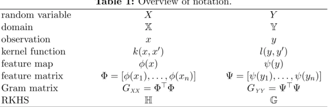
Figure 1:a) Propagation of the initial densityp0 by the Perron–Frobenius operator, where p1 = Pp0 and p2 = Pp1. b) Propagation of the embedded density µ0 by the embedded Perron–Frobenius operator, whereµ1 =PEµ0 andµ2 =PEµ1. The dashed black lines show the invariant and embedded invariant density, respectively.
embeddingpt and then applying the embedded Perron–Frobenius operator to
PE(Ekpt) =PE Z k(x,·)pt(x) dx = Z PEk(x,·)pt(x) dx = Z EY|x[φ(Y)|X =x]pt(x) dx = Z Z pτ(y |x)φ(y) dy pt(x) dx = Z k(y,·) Z pτ(y|x)pt(x) dxdy.
For the empirical estimates, the commutativity can be seen as follows: Letpt be a prob-ability density, then the empirical estimate of the kernel mean embedding is µbt = n1Φ1. Applying PbE yields
b PEµtb =
1
nCbYXCbXX−1Φ1= n1ΨΦ>(ΦΦ>)−1Φ1= n1Ψ1=µtb+τ.
That is, we obtain the empirical estimate of the mean embedding of the density pt+τ. In the last step, we again used the identity Φ(Φ>Φ)−1= (ΦΦ>)−1Φ.
Example 4.5. Let us consider the Ornstein–Uhlenbeck process from Example 3.4. We choose τ = 12,α = 4, D = 14, and the Gaussian kernel with σ2 = 12. Figure 1a shows the piecewise constant initial probability densityp0pushed forward by the Perron–Frobenius op-erator, Figure1b the embedded initial densityµ0 pushed forward by the embedded Perron–
Frobenius operator. N
The Perron–Frobenius operatorP maps densitiespt∈L1 topt+τ ∈L1, while the embed-ded Perron–Frobenius operator PE, given by the conditional mean embedding UY|X, maps
embedded densities µt ∈ H to µt+τ ∈ H. Thus, the conditional mean embedding plays a
similar role as the classical Perron–Frobenius operator in that it pushes forward—in this case: embedded—densities. Note that if we embed an eigenfunction ofP, we automatically obtain an eigenfunction ofPE. This is due to the linearity of the integral.
4.3 Kernel Koopman Operator
The Koopman operatorK applied to an observablef evaluated at xresults in the expecta-tion off when starting in xand evolving the system for time τ. Analogously to the kernel Perron–Frobenius operator, we now introduce the corresponding kernel Koopman opera-tor, denoted by Kk. That is, we assume that the observables and the observables mapped forward by the Koopman operator are elements ofH. From Proposition2.11, it follows that
Kk=C−1
XXCXY
and thus for f ∈H that
Kkf(x) =CXX−1CXYf, k(x,·)
=hf, PEk(x,·)i.
Alternatively, the kernel Koopman operator can be derived using the reproducing property directly: Kkf(x) = Z pτ(y|x)f(y) dy= Z hf, k(y,·)ipτ(y |x) dy = f, Z k(y,·)pτ(y |x) dy =hf, PEk(x,·)i. The empirical estimate of the Koopman operator is then given by
b
Kk=CbXX−1CbXY = (ΦΦ
>)−1(ΦΨ>) = ΦG−1
XXΨ
>.
Example 4.6. Let us approximate the kernel Koopman operator associated with the system defined in Example 3.6 using the kernel from Example 2.2. Generating 10000 test points xi sampled from a uniform distribution on X = [−2,2]×[−2,2] and the corresponding
yi=F(xi) values, we can compute the empirical estimator
b Kk=CbXX−1CbXY = ΦΦ >−1 ΦΨ> = ΨΦ+> ∈R6×6.
Here,+ denotes the pseudoinverse. The dominant eigenvalues and right eigenvectors as well as the corresponding eigenfunctions are given by
λ1 = 1.0, v1= [ 1 0 0 0 0 0 ]>, ϕ1(x) =hv1, φ(x)i= 1, λ2 = 0.8, v2= [ 0 0.7071 0 0 0 0 ]>, ϕ2(x) =hv2, φ(x)i ≈x1, λ3 = 0.7, v3= [ 0 0 0.7071 1 0 0 ]>, ϕ3(x) =hv3, φ(x)i ≈x2+x21. This is in good agreement with the analytically computed results. The eigenfunctions are clearly inHsince they can be written as linear combinations ofφ(xi) for appropriately chosen
xi, e.g., v2 =φ [14,0]>
−φ [−1 4,0]
>
. The subsequent eigenvalues and eigenfunctions are simply products of the eigenvalues and eigenfunctions listed above, see Example3.6. Note, however, that other than ϕ4 further products of eigenfunctions cannot be represented as functions inHanymore since the feature space does not contain polynomials of order greater
The approach to obtain an approximation of transfer operators from data as described in the above example is also referred to as EDMD (Williams et al.,2015a,Klus et al., 2016). The data matrices are embedded into a typically high-dimensional feature space, given, for instance, by monomials up to a certain order, which corresponds to the feature space of a polynomial kernel. Details regarding the relationships with other methods can be found in Section4.7and further examples in Section 5.
4.4 Embedded Koopman Operator
If we want to embed the Koopman operator in the same way as the Perron–Frobenius operator, we need to introduce embedded observables first, which can be interpreted as the counterpart of the mean embedding of distributions. Letf:X→Rbe an observable of the system. We define ν := Ekf to be the embedded observable. Given a set of training data, the empirical estimateνbof the embedded observable is given by
b ν = 1 n n X i=1 φ(xi)f(xi) = 1 n n X i=1 k(xi,·)f(xi) = 1 nΦf ,b
wherefb= [f(x1), . . . , f(xn)]> contains the values of the observable evaluated at the
train-ing data points. Note that the data points do not have to be drawn from a particular probability distribution. Alternatively, we could perform regression to approximate the observablef by an element fe∈H and then compute the integral.
Remark 4.7. Letνbe the embedding of the observablefwith respect to the kernelkand let pbe a density lying in the RKHSHspanned byk. Thenhν, piH=Rf(x)hk(x,·), piHdx= R
p(x)f(x) dx.
This result is an analogue of what has been attained previously for the kernel mean embedding of distributions, which also allows the representation of integration as an inner product in the RKHS, see Remark 2.6. Note that when using embedded distributions we have to assume that the observable is in H, while when using embedded observables we
assume the relevant density to be in H. One possible use of embedded observables arising
from Remark4.7is when one is unsure of the RKHS an observable lies in, while the RKHS of the density of interest is given. Another might be that by embedding the observable instead of the distribution one can take advantage of a smoother RKHS.
Analogously to the embedded Perron–Frobenius operator, we define the embedded Koop-man operator by KE =CXYCXX−1.
Proposition 4.8. Let νt:=Ekft be the embedded observable. Then the diagram L∞3ft νt∈H L∞3ft+τ νt+τ ∈H Ek K KE Ek is commutative.
As for P, embedding an eigenfunction of K results in an eigenfunction of KE. For the kernel Koopman operator Kk, the commutativity can be seen as follows: Assume that the observable is given by ft ∈H. Thus, Kkft = CXX−1CXYft, while the embedding of ft results
inνt=CXXft. ApplyingKE, this results in
KE(Ekft) =CXYCXX−1CXXft=CXXCXX−1CXYft=Ek(Kkft).
Proposition 4.9. The empirical estimate KbE of the embedded Koopman operator KE can be written as KbE = ΦAΨ>, where A is a real matrix. Estimates for A are given by A1 = GYXG−XX1G
−1
YX and A2 =GYYG−XY1G
−1
YX.
Proof. The proof is analogous to the proof of Proposition4.3.
Example 4.10. Let us consider again the system from Example 3.6whose eigenfunctions ϕ1,ϕ2, andϕ3we estimated numerically in Example4.6using the kernel from Example2.2. Computing the corresponding embedded eigenfunctions analytically, we obtain the (properly rescaled) functionsν1,ν2, andν3and associated vector representationsw1,w2, andw3, given by λ1 = 1.0, w1= [ 3 0 0 4 0 4 ]>, ν1(x) = 3 + 4x21+ 4x22, λ2 = 0.8, w2= [ 0 1 0 0 0 0 ]>, ν2(x) = √ 2x1, λ3 = 0.7, w3= [ 1 0 √ 2 125 0 43]>, ν3(x) = 1 + 2z2+125z21+43z22.
The vectorsw1,w2, andw3 are indeed eigenvectors of the matrixKbE =CbXYCbXX−1
correspond-ing to the eigenvaluesλ1,λ2, and λ3. N
4.5 Relationships between Operators
Overall, we derived four different operators that can be written in terms of the covariance and cross-covariance operators introduced in Section 2.
Kernel operator Embedded operator Perron–Frobenius Pk=C −1 XXCYX ≈ΨAΦ> PE =CYXC −1 XX ≈ΨG−1 XXΦ > Koopman Kk=C −1 XXCXY ≈ΦG−XX1Ψ > KE =CXYCXX−1 ≈ΦA>Ψ>
We can express the kernel Perron–Frobenius operator using the embedded Koopman oper-ator and the kernel Koopman operoper-ator using the embedded Perron–Frobenius operoper-ator—or mean embedding—via
Pkp(x) =hPkp, k(x,·)i
H =hp,KEk(x,·)iH,
Kkf(x) =hKkf, k(x,·)iH=hf, PEk(x,·)iH.
That is, Pk and KE as well as Kk and PE are adjoint to each other with respect to the inner product in H. This is also reflected in the empirical estimators. Here, A is either
A1 =G−XY1G
−1
XXGXY orA2 =G−XY1G
−1
4.6 Eigendecomposition of RKHS Operators
If the feature space is finite-dimensional and known explicitly, we can compute eigenfunc-tions as shown in Example 4.6, provided that the dimension of the feature space is small enough so that the resulting eigenvalue problem can still be solved numerically. The advan-tage of this approach is that the matrix size does not depend on the number of test pointsn. As described above, this approach converges to a Galerkin approximation of the respective operator for n→ ∞. The basis functions for the Galerkin ansatz are given by the feature map.
Now, we want to consider also the cases where the dimension of the feature space is larger than the number of test points or where the feature space is even infinite-dimensional. Let S = ΥBΓ> be a Hilbert–Schmidt operator mapping from H to itself, with Υ =
[k(z1,·), . . . , k(zn,·)], Γ = [k(z10,·), . . . , k(zn0,·)], and B ∈ Rn×n for some n. Assume fur-ther that Sn
i=1{zi, zi0} contains only pairwise different objects. Then the eigenvalues and eigenfunctions ofS can be computed from eigenvalues and eigenvectors of GΓΥB orB GΓΥ,
whereGΓΥ = Γ
>Υ.
Proposition 4.11. The Hilbert–Schmidt operatorS= ΥBΓ> has an eigenvalueλ6= 0with corresponding eigenfunction
υ= Υv
if and only ifvis an eigenvector ofB GΓΥ associated with λ. Similarly, S has an eigenvalue
λ6= 0 with corresponding eigenfunction
γ = ΓG−ΓΓ1v.
if and only if v is an eigenvector of GΓΥB.
Proof. Letυ= Υv be an eigenfunction ofS associated withλ. Then
Sυ=λυ ⇔
ΥB GΓΥv=λΥv ⇔
B GΓΥv=λv.
For the second part, letγ = ΓG−ΓΓ1v be an eigenfunction ofS. Then
Sγ =λγ ⇔ ΥB GΓΓG −1 ΓΓ v=λΓG −1 ΓΓ v ⇔ GΓΥBv=λv.
While these eigendecomposition derivations are the most elegant, other derivations exist. We conjecture that the eigenfunction expressions would coincide when taking the infinite-dimensional limit in the number of data pointsn(and thus in the size ofB, Υ, and Γ).
Setting Υ = Φ and Γ = Ψ or Υ = Ψ and Γ = Φ as well as B = A or B = A>, we thus obtain eigendecomposition expressions for all empirical operator estimates listed in Section4.5. In particular, let P∗ = ΨBΦ>. Then we need to solve the eigenvalue problem GXYBv=λv (which reduces toG−XX1GXYv=λv forPk with the estimator B =A1). We obtain an eigenfunction ofP∗ asϕ= ΦG−XX1v. For the Koopman operators, letK∗ = ΦBΨ
a) b)
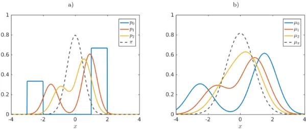
Figure 2:a) Dominant eigenfunctions of the Perron–Frobenius operatorP associated with the Ornstein–Uhlenbeck process. b) Dominant eigenfunctions of the Koopman operatorK. The solid lines are the numerically computed and the dotted lines the analytically computed eigenfunctions. Also the numerically computed eigenvalues agree with the analytically com-puted values.
Then we solve B GXYv = λv (i.e., G
−1
XXGYXv = λv for Kk). We get the eigenfunction ϕ= Φv. We will use these methods, which are consistent with the derivations in Williams et al. (2015a),Klus et al.(2018), for the experiments in Section 5.
Example 4.12. Let us analyze the Ornstein–Uhlenbeck process introduced in Example3.4. We use again τ = 12, α = 4, and D = 14 and generate 5000 uniformly distributed test points in [−2,2]. Furthermore, we use the Gaussian kernel with σ2 = 0.3. Applying our eigendecomposition result to the kernel Perron–Frobenius operator—since the test points are distributed uniformly, we obtain Pk, see Corollary 4.2—and kernel Koopman operator yields the results shown in Figure 2. This special case is equivalent to the kernel EDMD method. A similar experiment using conventional EDMD with a basis comprising monomials
is described in Klus et al.(2017). N
More complex examples from various application areas and different use cases will be discussed in Section5.
4.7 Relationships with Other Methods
There are several existing methods such as time-lagged independent component analysis (TICA) (Molgedey and Schuster,1994,P´erez-Hern´andez et al.,2013),dynamic mode decom-position (DMD) (Schmid,2010, Tu et al.,2014), and their respective generalizations—the aforementioned VAC and EDMD—to approximate transfer operators and their eigenvalues, eigenfunctions, and eigenmodes. Although developed independently from each other, these methods are strongly related as shown inKlus et al.(2017). Our methods subsume existing ones and thereby provide a unified framework for transfer operator approximation using RKHS theory.
4.7.1 TICA and DMD
TICA can be used to separate superimposed signals (Molgedey and Schuster,1994), solving the so-calledblind source separation problem, and also for dimensionality reduction (P´ erez-Hern´andez et al.,2013), by projecting a high-dimensional signal onto the main TICA coordi-nates (see Section5for an example). The method aims to find the time-lagged independent components that are uncorrelated and maximize the autocovariances at lag timeτ. Given again training dataDXY ={(x1, y1), . . . ,(xn, yn)}, wherexi=Xtiandyi =Xti+τ, we define
the associated data matricesX,Y∈Rd×n by
X= x1 · · · xn and Y= y1 · · · yn .
By setting k(x, x0) = x>x0 and l(y, y0) = y>y0, the eigenvalue problem for the Koopman operator reduces to the standard eigenvalue problem
b C−1
XXCbXYξ=λ ξ,
whereCbXXandCbXY denote the covariance and cross-covariance matrices, respectively, defined
byCbXX = 1nXX>andCbXY = n1XY>. The resulting eigenvectors are defined to be the TICA
coordinates.
DMD is frequently used for the analysis of high-dimensional fluid flow problems (Schmid,
2010). The DMD modes correspond to coherent structures in these flows. The derivation is based on the least-squares minimization problemkY−MXkF, whose solution is given by
M =YX+= YX>
XX>−1
=CbYXCbXX−1.
Eigenvectors of this matrix are then called DMD modes. Equivalently, the DMD modes can be interpreted as the left eigenvectors of the TICA matrixCbXX−1CbXY. More details on the
relationships between TICA and DMD can be found inKlus et al.(2017). As shown above, both TICA and DMD can be obtained as special cases of our algorithms.
4.7.2 VAC and EDMD
For a given set of basis functions φ1, . . . , φr, we define the vector-valued function φ = [φ1, . . . , φr]>:Rd→ Rr. In the context of the kernel-based methods introduced above, the
function φ corresponds to an explicitly defined feature map. This results in the feature matrices Φ,Ψ∈Rr×n, given by
Φ =φ(x1) · · · φ(xn)
and Ψ =φ(y1) · · · φ(yn)
.
Note that the same basis functions—and thus the same kernel—are used forxandy, a gen-eralization of this approach can be found inWu and No´e (2017). VAC and EDMD, which are equivalent for reversible dynamical systems, can be understood as nonlinear extensions of TICA and DMD, respectively. Both methods utilize the transformed data matrices Φ and Ψ for an explicitly given set of basis functions. VAC uses the matrixCbXX−1CbXY as an
approx-imation of T (which is equivalent to K for a reversible system) to compute eigenfunctions. Similarly, EDMD considers the matrix CbYXCbXX−1, which can be interpreted as a least-square
way, we obtainCbXYCbXX−1 for the Perron–Frobenius operator.) By defining the kernelskandl
explicitly ask(x, x0) =φ(x)>φ(x0) andl(y, y0) =φ(y)>φ(y0) for some finite-dimensional fea-ture spacesHand G, we can also see the close relationship between the methods described
in this paper and VAC and EDMD. Given a finite-dimensional feature space,CbXX = n1ΦΦ>
and CbYX = n1ΨΦ
> can be computed explicitly. See also Example4.6and Section 5.
4.7.3 Kernel TICA and Kernel EDMD
The advantage of our method compared to VAC and EDMD is that the eigenvalue problem can be expressed entirely in terms of the Gram matrices GXX, GXY, GYX, andGYY. The
transformed data matrices Φ and Ψ need not be computed explicitly. This also allows us to work implicitly with infinite-dimensional feature spaces. Kernel-based variants, based on algebraic transformations of the conventional counterparts, of TICA and EDMD have also been proposed inSchwantes and Pande (2015),Williams et al. (2015b), Klus et al.(2018). Similar to VAC, kernel TICA is based on a variational approach and requires reversibility, whereas kernel EDMD is also defined for non-reversible systems. Although kernel TICA and kernel EDMD are generalizations of different methods—TICA is related to DMD and VAC to EDMD—, the resulting methods are strongly related again. In Schwantes and
Pande (2015), conventional TICA is first implicitly extended to VAC and then to kernel
TICA, whereas the derivation of kernel EDMD explicitly uses the EDMD feature space representation, see also Klus et al.(2018).
5 Experiments
We will briefly show how the methods introduced above can be used to analyze dynamical systems and time-series data. In the first example, we analyze two simple molecular dynam-ics related problems using methods that correspond to EDMD and TICA. The second exam-ple illustrates that the kernel-based reformulations can also be applied to high-dimensional video data. The third example shows another new application, the analysis of text data. Further molecular dynamics examples can be found inN¨uske et al. (2014), McGibbon and Pande(2015),Schwantes and Pande(2015),Klus et al.(2016,2017,2018) and applications in fluid dynamics, e.g., inBudiˇsi´c et al.(2012),Williams et al.(2015b),Rowley et al.(2009).
5.1 Molecular Dynamics
In this section, we apply the proposed techniques to extract meta-stable sets and to reduce the dimension of time series data.
5.1.1 Meta-stable sets
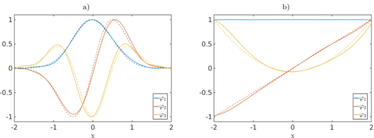
As a first example, let us illustrate how the eigendecomposition of Kk—for an explicitly defined feature space, which corresponds to EDMD as described above—can be used for molecular dynamics applications. We consider a simple multi-well diffusion process given by a stochastic differential equation of the form
dXt=−∇V(Xt) dt+
√
a) b)
Figure 3: a) Potential V associated with the multi-well diffusion process. b) Partitioning of the state space based on the dominant eigenfunctions of the Koopman operator.
whereV is the potential,D=β−1 again the diffusion coefficient, andWta standard Wiener process. The potential, shown in Figure3a, is given by
V(x) = cos (karctan(x2, x1)) + 10 q
x21+x22−1
2
,
see also Bittracher et al. (2017). We set k = 5. A particle will typically spend a long time in one of the wells and then jump to one of the adjacent wells. The transitions between the wells are rare events. Thus, this system exhibits metastable behavior and the five metastable sets—which are encoded in the five dominant eigenfunctions of the transfer operators associated with the system—correspond to the five wells of the potential.
We use a 50×50 box discretization of the domain X= [−2,2]×[−2,2] to define a basis
containing 2500 radial basis functions ki(x, ci) = exp(−21σ2 kx−cik2) whose centers ci are the centers of the boxes. This defines a kernel
k(x, x0) = 2500 X i=1 ki(x, ci)ki(x0, ci) = 2500 X i=1 exp − 1 2σ2 kx−cik2+ x0−ci 2 .
Furthermore, we choose the lag timeτ = 0.2 and σ2 = 0.9. We generate 250000 uniformly distributed test pointsxi∈Xand solve the initial value problem with the Euler–Maruyama
method to obtain the correspondingyi values. We then compute the eigenvalues and eigen-functions of the Koopman operator Kk. There exist five dominant eigenvalues close to one and then there is a spectral gap between the fifth and sixth eigenvalue. We apply ak-means clustering to the dominant eigenfunctions to obtain the partitioning of the domain into the five metastable sets shown in Figure3b. There are more sophisticated techniques to iden-tify the metastable sets based on the eigenfunctions, but the example illustrates the basic workflow.
a) b)
Figure 4: a) Original data set. b) Projection onto the TICA coordinates. Only the first two variables corresponding to the dominant eigenvalues exhibit metastable behavior.
5.1.2 Dimensionality reduction and blind source separation
Another use case of the methods introduced above is dimensionality reduction. Before methods to compute eigenfunctions of transfer operators such as EDMD or VAC can be applied to high-dimensional systems, the data often needs to be projected onto a lower-dimensional subspace first. This can be accomplished by approximating the eigenfunctions of the Koopman operator Kk using a linear kernel (i.e., TICA, see Section 4.7). Let us consider the simple data set x ∈ R4×10000 shown in Figure 4a. From this data set, we extract X = [x1, . . . , x9999] and Y = [x2, . . . , x10000], where xi denotes the ith column vector ofx. Applying TICA, we see that there are two dominant eigenvalues close to 1, the other two are close to 0. This indicates that two of the four variables exhibit metastable behavior. Projecting the data onto the TICA coordinates results in the trajectories shown in Figure4b. The first two new variables corresponding to the dominant eigenvalues contain the metastability, while the other two variables contain just noise. (In fact, this is how the data set was constructed.) Since we are only interested in the slow metastable dynamics, we can neglect the last two variables and thus reduce the state space. At the same time, we can view the projection onto eigenfunction coordinates as the unmixing of previously mixed signal sources. Thus, our methods can be used for solving blind source separation problems.
5.2 Movie Data
Let us analyze a simple movie showing a pendulum1. We want to analyze this data set using the eigendecomposition ofKk for a Gaussian kernelk(corresponding to kernel EDMD). To this end, we convert each 576×720 RGB video frame to a grayscale intensity image—all intensities are between 0 and 1—and define a kernel k(x, y) = exp − 1
2σ2 kx−ykF
, with
1ScienceOnline: The Pendulum and Galileo (
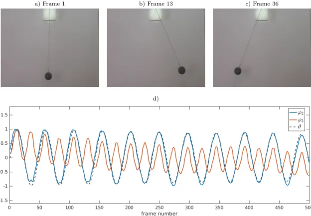
a) Frame 1 b) Frame 13 c) Frame 36
d)
Figure 5:a) No angular displacement. b) Maximum displacement right-hand side. c) Max-imum displacement left-hand side. d) Values of the normalized eigenfunctions ϕ2 and ϕ3 for each frame. The eigenfunctions encode the frequency of the pendulum. The frames 13 and 36 correspond to the first maximum and minimum of the eigenfunctionϕ2. The period of ϕ3 is twice the period of ϕ2. The black dashed line shows the angular displacement ϑ (rescaled for the sake of comparison) obtained by a numerical simulation of the pendulum. The dominant eigenfunction parametrizes the angular displacement. The video snapshots are reproduced with the kind permission of ScienceOnline.
σ2 = 500. Here, k·k
F denotes the Frobenius norm. It would also be possible to use the RGB signal directly, e.g., by definingkRGB(x, y) =k(xR, yR) +k(xG, yG) +k(xB, yB), i.e., each primary color is compared separately. The video comprises 501 frames so thatX, Y ∈ R576×720×500. That is, the data sets are now tensors of order three. Analogously, we could
reshape the snapshot matrices into vectors. We choose the regularization parameter ε = 0.05. Thus, for our analysis, we have to solve the eigenvalue problem (GXX+ε In)−1GYXv=
λ v to obtain eigenfunctions ofKk.
The values of the resulting nontrivial dominant eigenfunctions ϕ2 and ϕ3 evaluated for each frame are shown in Figure5. The first nontrivial eigenfunction encodes the frequency of the pendulum and the second eigenfunction twice the frequency. As a result, we could now sort the frames according to the angular displacement of the pendulum using the eigen-functions. The example shows that even for high-dimensional problems the kernel-based methods are able to extract relevant information about the global dynamics. The frames attaining maxima and minima of the eigenfunctions provide a summary of the video using
typical (but maximally different) frames. This use of our methods resemblesdeterminantal point processes as applied to data summarization (Kulesza and Taskar,2012).
For this simple example, we used the raw video data. For more complex systems, pre-processing steps might be beneficial, e.g., mean subtraction, Sobel edge detection, or more sophisticated feature detection approaches such as SIFT or HOG (Bo et al.,2010). In this way, it would be possible to track features of images over time. Another potential appli-cation that we considered but did not include here is the analysis of persons walking or running. The eigenfunctions then describe the gait pattern and gait velocity.
5.3 Text Data
In this section, we show how the eigendecomposition of the kernel Perron–Frobenius operator with respect to the invariant density, denoted by Tk, can be used for non-vectorial data. Consider the following scenario: Given a collection of text documents, erase all words not contained in a predefined vocabulary. Of the remaining words, one word (denoted by yi) following another (denoted byxi) is considered to be its time evolved version or successor. The lists of all such wordsxi and yi are denoted byX and Y, respectively. We choose the vocabulary shown in Table2 and collect 1000 word pairs from news articles. Typically, the same word or related words are used several times within one article, but words related to other topics are rarely mentioned. Since we consider the sequence of articles as one long document2, transitions occur, for instance, when one article ends and the next one about a different topic starts, when different topics are mixed, or when words such asstate or cell are used in a different context. These are the rare transitions that are similar to the jumps between the wells in the molecular dynamics example. Although this is a slightly artificial example, it illustrates how to extend transfer operator approaches to new domains where only a similarity measure given by a kernel is available.
Table 2: Predefined set of keywords.
browser cell computer damage department disease e-mail election hurricane internet midterm president rain science state stem storm tablet therapy weather
We generate the Gram matrices GXY and GXX and compute eigenfunctions of the
op-erator Tk. Here, [GXY]ij = k(xi, yj), where xi is the ith word in X and yj the jth word
inY. Correspondingly, GXX is the standard Gram matrix. Moreover, k is the text kernel
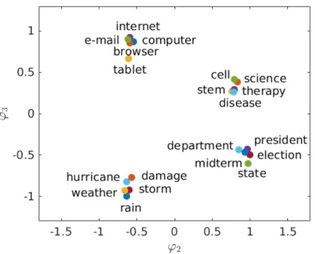
proposed in Lodhi et al.(2002)3. We compute again the leading nontrivial eigenfunctions ϕ2 andϕ3 and use the the eigenfunctions as coordinates. The results are shown in Figure6. Note that the words are not clustered based on string kernel similarity but on proximity in the document collection. Words that often occur together are grouped into clusters. For this simple example, it would also have been possible to assign each word a distinct num-ber and to generate a Markov state model by approximating the transition probabilities
2
Parts of the same articles are used several times to increase the size of the data set, this is thus a synthetic example, mainly to illustrate the concept.
3We use theString Kernel Software implementation (
Figure 6:Topic modeling by clustering using on the dominant eigenfunctions. Words that are found in close proximity represent a topic. Our method identified four topic clusters: information technology, medicine, weather, and politics.
between words. The eigenvectors of the Markov matrix would then lead to a similar clus-tering. The text kernel, however, takes into account string similarity. This is important to account, for example, for grammatical variations reflected in word form (green vs.greener) and misspellings (lovevs.loove) without necessarily resorting to lemmatizing, stemming, or other normalization techniques. Another possibility here would be to design linguistically informed string kernels. In German for example, aVisumantrag (visa application) is more similar to Antrag (application) than to Visum. A string kernel taking this into account would instantly be reflected in the word clusters discovered by our method, which could never be achieved when using a pure Markov state model.
Compared to latent Dirichlet allocation (LDA) (Blei et al.,2003), our method of uncov-ering topics in texts differs in several respects. First of all, LDA is derived as a Bayesian model, while our method can be considered frequentist. Second, LDA makes a bag-of-words assumption, i.e., the order of words in texts is not taken into account. Our method, on the other hand, relies first and foremost on word order. Third, the semantic content of words in LDA could be summarized as a real vector using their frequency in topics, while a clustering of words into topics is the primary object of interest. Our method, on the other hand, produces a semantic word representation, the eigenfunction values of a word, while a clustering into topics can be implemented as a postprocessing step. This is an interesting application warranting further research that follows directly from our general principle of decomposing an RKHS operator.
6 Conclusion
We have shown how to extend transfer operator theory to reproducing kernel Hilbert spaces and illustrated similarities with the conditional mean embedding framework. While the con-ventional transfer operator propagates densities, the kernel mean embedding can be viewed as an operator that propagates embedded densities. Moreover, we have highlighted rela-tionships between the covariance and cross-covariance operator based methods to obtain empirical estimates of the conditional mean embedding and other well-known methods for the approximation of transfer operators developed by the dynamical systems, molecular dy-namics, and fluid dynamics communities. One main benefit of purely kernel-based methods is that these methods can be applied to non-vectorial data such as strings or graphs, enabling the analysis of many (wide-sense) stationary processes. We demonstrated the efficiency and versatility of these methods using guiding examples as well as simple molecular dynamics applications, video data, and text data. Future work includes applying the aforementioned kernel-based methods to more realistic data sets. In particular the analysis of real-world text data and more complicated video data, potentially in combination with machine learn-ing based preprocesslearn-ing approaches, will be a challenglearn-ing task. An open question is also the convergence of the RKHS operator to the actual transfer operator. Furthermore, the influence of the kernel itself, the regularization parameter, and the number of test points on the accuracy of the eigenfunction approximations is not clear yet. These questions will be addressed in future work. Another extension of the framework presented within this paper would be to use singular value decompositions instead of eigenvalue decompositions for the transfer operator representations. The resulting methods could then also be applied to problems where the spaces Xand Yare different.
Acknowledgements
This research has been partially funded by Deutsche Forschungsgemeinschaft (DFG) through grant CRC 1114“Scaling Cascades in Complex Systems”. Krikamol Muandet acknowledges fundings from the Faculty of Science, Mahidol University and the Thailand Research Fund (TRF).
A Analytical Mean Embeddings and Its Inversion
If the function is given by a sum of Gaussians and the kernel is Gaussian or Student-t, the embedding and its inverse can be computed analytically.
A.1 Gaussian functions, Gaussian kernels
Let k(x, x0) be the kernel given by the normalized d-dimensional Gaussian density with covariance Σk, mean x0, and evaluation at point x. Let g(·) = P∞
i=1aiN(·;µi,Σi), where theN(·;µi,Σi) ared-dimensional multivariate Gaussian densities and ai ∈R. Then
(Ekg)(·) = ∞
X
i=1