A linear-time algorithm for maximum-cardinality matching on cocomparability graphs.

Deposited in DRO:

04 January 2019

Version of attached le:

Published Version

Peer-review status of attached le:

Peer-reviewed

Citation for published item:

Mertzios, G.B. and Nichterlein, A. and Niedermeier, R. (2018) 'A linear-time algorithm for

maximum-cardinality matching on cocomparability graphs.', SIAM journal on discrete mathematics., 32 (4). pp. 2820-2835.

Further information on publisher's website:

https://doi.org/10.1137/17M1120920

Publisher's copyright statement:

c

2018 SIAM.

Additional information:

Use policy

The full-text may be used and/or reproduced, and given to third parties in any format or medium, without prior permission or charge, for personal research or study, educational, or not-for-prot purposes provided that:

• a full bibliographic reference is made to the original source

• alinkis made to the metadata record in DRO

• the full-text is not changed in any way

The full-text must not be sold in any format or medium without the formal permission of the copyright holders.

A LINEAR-TIME ALGORITHM FOR MAXIMUM-CARDINALITY

MATCHING ON COCOMPARABILITY GRAPHS\ast

GEORGE B. MERTZIOS\dagger , ANDR \'E NICHTERLEIN\dagger \ddagger , AND ROLF NIEDERMEIER\ddagger

Abstract. Finding maximum-cardinality matchings in undirected graphs is arguably one of the

most central graph problems. For generalm-edge andn-vertex graphs, it is well known to be solvable inO(m\surd n) time. We present a linear-time algorithm to find maximum-cardinality matchings on

cocomparabilitygraphs, a prominent subclass of perfect graphs that strictly contains interval graphs

as well as permutation graphs. Our greedy algorithm is based on the recently discoveredLexicographic

Depth First Search(LDFS).

Key words. greedy algorithms, Lexicographic Depth First Search, perfect graphs, interval

graphs

AMS subject classifications. 05C85, 05C70, 05C17

DOI. 10.1137/17M1120920

1. Introduction. The problem Matching (or Maximum-Cardinality

Matching) is, given an undirected graph, to compute a maximum-cardinality set of

disjoint edges. Matchingis arguably among the most fundamental graph-algorithmic primitives that can be computed in polynomial time. More specifically, the asymp-totically fastest known algorithm for computing a maximum-cardinality matching (subsequently called maximum matching) on an n-vertex and m-edge graph runs

in O(m\surd n) time [44]. No faster algorithm is known, even when the given graph is

bipartite [24]. Improving this running time, either on general graphs or on bipartite graphs, resisted decades of research. In terms of approximation, it is known that

the O(m\surd n) algorithm of Micali and Vazirani [44] implies a (1 - \epsilon )-approximation

computable in O(m\epsilon - 1) time [13]. For the weighted case, Duan and Pettie [13] pro-vided a linear-time algorithm that computes a (1 - \epsilon )-approximate maximum-weight matching (the constant running time factor depending on \epsilon is \epsilon - 1log(\epsilon - 1)). In this work we take a route different from approximation and identify a large graph class, namely cocomparability graphs, on which we show that an optimal solution can be computed in linear time.

Identifying more efficiently solvable special cases for finding maximum match-ings has quite some history. Yuster [56] developed an algorithm with running time O(rn2logn), where r denotes the difference between maximum and minimum vertex degree of the input graph. Moreover, there are (quasi)linear-time algorithms for computing maximum matchings in several special classes of graphs, including in-terval graphs [30], convex bipartite graphs [51], strongly chordal graphs [10], and chordal bipartite graphs [3]. We refer the reader to Table 1 for a more thorough overview, also including results with superlinear running times. See Figure 1 for an

\ast _{Received by the editors March 14, 2017; accepted for publication (in revised form) October 2,}

2018; published electronically December 4, 2018.

http://www.siam.org/journals/sidma/32-4/M112092.html

Funding: The first author was partially supported by the EPSRC grant EP/P020372/1. The

second author was supported by a postdoc fellowship of the German Academic Exchange Service (DAAD) while at Durham University.

\dagger _{Department of Computer Science, Durham University, DH1 3LH Durham, UK}

(george.mertzios@durham.ac.uk).

\ddagger _{Algorithmics and Computational Complexity, Faculty IV, TU Berlin, 10587 Berlin, Germany}

(andre.nichterlein@tu-berlin.de, rolf.niedermeier@tu-berlin.de).

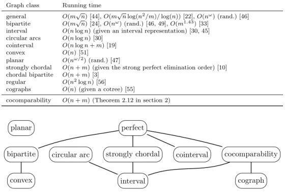
Table 1

Fastest algorithms for Matchingon special graph classes;\omega <2.373is the matrix

multiplica-tion exponent, that is, twon\times nmatrices can be multiplied inO(n\omega _)time.

Graph class Running time

general O(m\surd n) [44],O(m\surd nlog(n2_{/m)/log(n)) [22],O(n}\omega _{) (rand.) [46]}

bipartite O(m\surd n) [24],O(n\omega ) (rand.) [46, 49],O(m1.43) [33] interval O(nlogn) (given an interval representation) [30, 45] circular arcs O(nlogn) [30]

cointerval O(nlogn+m) [19] convex O(n) [51]

planar O(n\omega /2) (rand.) [47]

strongly chordal O(n+m) (given the strong perfect elimination order) [10] chordal bipartite O(n+m) [3]

regular O(n2_{logn) [56]}

cographs O(n) (given a cotree) [55]

cocomparability O(n+m) (Theorem 2.12 in section 2)

planar perfect

bipartite circular arc strongly chordal cointerval cocomparability

convex interval cograph

Fig. 1. Overview of most of the graph classes mentioned in Table 1. An edge indicates that

the class above strictly contains the class below.

overview concerning the containment relation between the graph classes.

A graphGis acocomparabilitygraph if its complementGadmits a transitive ori-entation of its edges. These graphs (as well as their complements, i.e., comparability graphs) arise naturally in several real-world applications as they are closely related to

partially ordered sets (also referred to as posets). In particular, a given

cocompara-bility graphG, together with a transitive orientation of the edges of its complement G, can be equivalently represented by a poset. Cocomparability graphs have been the subject of intensive theoretical research [4, 6, 7, 11, 14, 15, 26, 27, 29, 39, 43]. On the one hand, cocomparability graphs naturally generalize well-studied graph classes such as interval and permutation graphs [2, 23],trapezoid (orbounded multitolerance) graphs [25, 28, 32, 36, 38, 52],parallelogram(orbounded tolerance) graphs [20, 41, 42],

triangle (or PI\ast ) graphs [5, 35], and simple-triangle (or PI) graphs [37, 53, 54]. On

the other hand, cocomparability graphs form an ``almost maximal"" subclass of perfect graphs [2].1 _{Since perfect graphs (as well as comparability graphs) properly contain}

bipartite graphs (for which improving the O(m\surd n) running time is a long-standing open question), it seems out of reach to obtain an algorithm for_Matchingwith linear running time on perfect graphs. Consequently, designing a linear-time algorithm for cocomparability graphs provides a sharp boundary betweenO(n+m)-time algorithms and the knownO(m\surd n)-time algorithms for_Matching.

1_{For an overview of the relation between graph classes see http://www.graphclasses.org/.}

Our contribution. In this paper we present a linear-time algorithm for_Matching

oncocomparability graphs. It is a simple greedy algorithm, referred to asRightmost

Matching (RMM), running on a specific vertex ordering. Essentially the same greedy approach was earlier considered by Dragan [12] in the context of greedy matchable graphs.2 _{The vertex ordering is obtained by using (as a preprocessing step) the}

recently discovered Lexicographic Depth First Search (LDFS) algorithm [8]. Inter-estingly it turns out that RMM computes in atrivial way a maximum matching on interval graphs, when applied on the standard interval graph vertex ordering.3 Note that the class of interval graphs is a strict subset of the class of cocomparability graphs. So far a similar phenomenon of extending an interval graph algorithm to cocomparability graphs by using an LDFS preprocessing step has also been observed for the _{Longest Path}problem [39], the _{Minimum Path Cover} problem [6], and

the_{Maximum Independent Set}problem [7]. Our results for the RMM algorithm,

adding to the previous results [6, 7, 39], provide evidence that cocomparability graphs present an ``interval graph structure"" when they are considered with an LDFS pre-processing step. This insight is of independent interest and might lead to new and more efficient combinatorial algorithms.

Preliminaries. We use standard notation from graph theory. In particular, all

paths we consider are simple paths. A matching in a graph is a set of pairwise disjoint edges. LetG= (V, E) be an undirected graph, and letM \subseteq E be a matching in G. A vertex v\in V is calledmatched with respect toM if there is an edge inM containing v; otherwise v is called free with respect to M. If the matching M is clear from the context, then we omit ``with respect toM."" Analternating path with respect toM is a path in Gsuch that every second edge of the path belongs toM.

Anaugmenting pathis an alternating path whose endpoints are free. It is well known

that a matchingM is maximum if and only if there is no augmenting path for it [31]. A graph G= (V, E) is an interval graph if we can assign to each vertex of Ga closed interval on the real line such that two vertices are adjacent inGif and only if the corresponding two intervals intersect. Acomparability graph is a graph whose edges can be transitively oriented; that is, if u\rightarrow v (the edge\{ u, v\} is oriented towardsv)

andv\rightarrow w, thenu\rightarrow w. Acocomparability graphGis a graph whose complementG

is a comparability graph. The class of interval graphs is strictly included in the class of cocomparability graphs [2]. Intuitively, we can transitively orient the ``nonedges"" of an interval graph, using the following ordering of nonintersecting intervals from left to right: Consider three intervalsIa, Ib, Ic in an interval representation of an interval

graph. IfIa lies completely to the left of Ib, andIb lies completely to the left ofIc,

then alsoIa lies completely to the left ofIc.

2. A linear-time algorithm for cocomparability graphs. To begin with,

we present in subsection 2.1 a simple greedy linear-time algorithm (called RMM) for computing a maximum matching M on interval graphs. Subsequently we provide in subsection 2.2 all necessary background on vertex orderings for cocomparability graphs and on the LDFS, which is needed for our algorithm on cocomparability graphs. Finally, as our central result, we prove in subsection 2.3 that the algorithm RMM actually works also for cocomparability graphs.

2_{Refer to Remark 2 in subsection 2.3 for a discussion about the subtle but important differences}

from our approach.

3_{This is the vertex ordering that results from sorting the intervals according to their left}

end-points. The RMM algorithm for interval graphs was discovered by Moitra and Johnson [45].

2.1. The greedy algorithm for interval graphs. Given an interval graphG withnvertices andmedges, we first compute inO(n+m) time an interval represen-tation of Gand, at the same time, we also sort the intervals according to their left endpoint [48]. The algorithm works as follows (cf. [30, 45]):

1. InitializeM =\emptyset and label all vertices as ``unvisited.""

2. Pick the unvisited vertex (interval) xwhich has the rightmost left endpoint among all currently unvisited vertices inG. Then, labelxas ``visited."" 3. Ifxhas at least one unvisited neighbor in G, then pick the unvisited

neigh-boryofxwhich has the rightmost left endpoint among all unvisited neighbors ofx. Then labely as ``visited"" and add the edge\{ x, y\} to M.

4. If there is still an unvisited vertex inG, then go to step 2. 5. ReturnM.

We call the above algorithmRightmost Matching(RMM). It can be executed inO(n+ m) time; with a simple exchange argument we can show that the matchingM returned by RMM is indeed maximum inG. This algorithm implicitly uses the following vertex ordering that characterizes interval graphs. It corresponds to sorting the intervals according to their left endpoints and can be computed inO(n+m) time fromG[48].

Lemma 2.1 (see [48]). G= (V, E)is an interval graph if and only if there exists

a vertex ordering \sigma of G (called an I-ordering) such that, for all x <\sigma y <\sigma z, if

\{ x, z\} \in E, then also \{ x, y\} \in E.

2.2. Cocomparability graphs and vertex orderings. Before we proceed

with our algorithm RMM and its analysis on cocomparability graphs (see subsec-tion 2.3), we now state vertex ordering characterizasubsec-tions of cocomparability graphs and of any vertex ordering that can result from an LDFS search on an arbitrary graph. The following vertex ordering characterizes cocomparability graphs [27].

Definition 2.2 (see [27]). Let G = (V, E) be a graph. An ordering \pi of the

verticesV is an umbrella-freeordering (or a CO-ordering) if for allx <\pi y <\pi z it

holds that if\{ x, z\} \in E, then\{ x, y\} \in E or\{ y, z\} \in E (or both).

Lemma 2.3 (see [27]). A graphG= (V, E)is a cocomparability graph if and only

if there exists an umbrella-free ordering \pi of V.

Umbrella-free orderings directly generalize I-orderings for interval graphs (see Lemma 2.1). It is worth noting here that, although there exists a linear-time al-gorithm tocomputean umbrella-free ordering\pi of a given cocomparability graph [34], the fastest known algorithm toverify that a given vertex ordering is indeed umbrella-free needs the same time as boolean matrix multiplication (Spinrad [50] discusses this issue). As an example, we illustrate in Figure 2 the cocomparability graph C6,

i.e., the complement of the cycle on six vertices. In this graph, it is straightforward to check by Definition 2.2 that the vertex ordering \pi = (b, d, c, f, e, a) is indeed an umbrella-free ordering.

In the following we present the notion of an LDFS ordering\sigma (see Definition 2.5) due to Corneil and Krueger [8]. This notion is based ongood triples andbad triples, which are defined next.

Definition 2.4 (see [8]). Let G = (V, E) be a graph and \sigma be an arbitrary

ordering of V. Let a, b, c \in V be three vertices such that a <\sigma b <\sigma c, \{ a, c\} \in E,

and \{ a, b\} \in / E. If there exists a vertex d such that a <\sigma d <\sigma b, \{ d, b\} \in E, and

\{ d, c\} \in /E, then(a, b, c)is a good triple; otherwise it is a bad triple.

Definition 2.5 (see [8]). Let G= (V, E)be a graph. An ordering \sigma of V is an

b

c

d

e

a

f

Fig. 2.The cocomparability graphG=C6, i.e., the complement of a cycle on six vertices. The

vertex ordering\pi = (b, d, c, f, e, a)is an umbrella-free ordering forG.

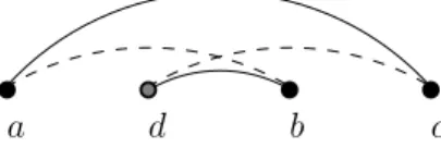
a

d

b

c

Fig. 3. A good triple (a, b, c) and its vertex d as in Definition 2.4, in the vertex ordering

\sigma = (a, d, b, c). The edges\{ a, c\} and\{ d, b\} are indicated with solid lines and the nonedges\{ a, b\} and

\{ d, c\} with dashed lines. Note that\{ a, d\} and\{ b, c\} can be edges or nonedges.

LDFS orderingif \sigma has no bad triple.

An example of a good triple (a, b, c) and the corresponding fourth vertex d is depicted in Figure 3. Now we present the generic LDFS algorithm (Algorithm 1) due to Corneil and Krueger [8]. LDFS runs on an arbitrary connected graphG, starting at a distinguished vertexu. It is a variation of the well-known Depth First Search (DFS) algorithm; the main difference is that LDFS assigns labels to the vertices and uses the lexicographic order over these labels as a tie-breaking rule. Briefly, it proceeds as follows. Initially, the label \varepsilon is assigned to every vertex. Then, iteratively, an unvisited vertex v with a lexicographically maximum label is chosen and removed from the graph. Ifvis chosen as theith vertex, then the label of each of its unvisited neighbors is being updated by prepending the digit i to it. Note that the digits in the label of any vertex are always in decreasing order. Hence all neighbors of the last chosen vertex have a lexicographically greater label than all its nonneighbors, and thus all vertices are visited in a depth first search order.

Algorithm 1. LDFS(G, u) [8].

Input: A connected graphG= (V, E) withnvertices and a vertexu\in V.

Output: An LDFS ordering\sigma u of the vertices ofG.

1: Assign the label\varepsilon to all vertices and mark all vertices as unnumbered 2: label(u)\leftarrow \{ 0\}

3: fori= 1 tondo

4: Pick an unnumbered vertex v with the lexicographically largest label

5: \sigma u(i)\leftarrow v \{ assign to vthe numberi;v is now numbered\}

6: foreach unnumbered vertexw\in N(v)do

7: prependito label(w)

8: return the ordering\sigma u= (\sigma u(1), \sigma u(2), . . . , \sigma u(n))

The execution of the LDFS algorithm is illustrated with the running example of Figure 2. In this example, suppose that the LDFS algorithm starts at vertex a. Suppose that LDFS chooses vertexc next. Now, ordinary DFS could choose eithere orf next, but LDFS has to choosee, sinceehas a greater label thanf (eis a neighbor of the previously visited vertexa). The next visited vertex has to beb, since it is the only unvisited neighbor of e. The vertex following b in the LDFS ordering \sigma a must

be f rather than d, since f has a greater label than d(f is a neighbor of vertex c which has been visited more recently thand's neighbora). Finally, LDFS visits the last vertexd, completing the LDFS ordering as \sigma a = (a, c, e, b, f, d).

It is important here to connect the vertex ordering \sigma u that is returned by the

LDFS algorithm (i.e., Algorithm 1) with the notion of an LDFS ordering, as defined in Definition 2.5. The next theorem due to Corneil and Krueger [8] shows that a vertex ordering \sigma of an arbitrary graph Gcan be returned by an application of the LDFS algorithm toG (starting at some vertexu ofG) if and only if \sigma is an LDFS ordering.

Theorem 2.6 (see [8]). For an arbitrary graphG= (V, E), an ordering\sigma ofV

can be returned by an application of Algorithm 1 to G if and only if \sigma is an LDFS

ordering.

In the generic LDFS, there can be some choices to be made at Line 4 of Algo-rithm 1. More specifically, at some iteration there may be two or more vertices that have the same label; in this case the algorithm must break ties and choose one of these vertices. Generic LDFS (i.e., Algorithm 1) allows an arbitrary choice here. We present in the following a special type of LDFS algorithm, called LDFS+ _(see

Al-gorithm 2 below), which chooses a specific vertex in such a case of equal labels, as follows. Along with the graphG= (V, E), an ordering\pi ofV is also given as input. The algorithm LDFS+_{operates exactly as a generic LDFS that starts at therightmost}

vertex ofV in the ordering\pi , with the only difference being that, in the case where at some iteration at least two unvisited vertices have the same label, LDFS+ _chooses

therightmost vertex among them in the input ordering\pi . The resulting ordering is

then denoted\sigma = LDFS+(G, \pi ).

Algorithm 2. LDFS+ (G, \pi ).

Input: A connected graphG= (V, E) withnvertices and an ordering\pi ofV.

Output: An LDFS ordering\sigma of the vertices ofG.

1: Assign the label\varepsilon to all vertices and mark all vertices as unnumbered 2: fori= 1 tondo

3: Pick the rightmost vertex v in \pi among the unnumbered vertices with the lexicographically largest label

4: \sigma (i)\leftarrow v \{ assign to vthe numberi;v is now numbered\}

5: foreach unnumbered vertexw\in N(v)do

6: prependito label(w)

7: return the ordering\sigma = (\sigma (1), \sigma (2), . . . , \sigma (n))

Consider our running example of Figure 2. In this graph G=C6, suppose that

LDFS+ _{is given as input the umbrella-free ordering \pi = (b, d, c, f, e, a). Then the}

ordering \sigma = LDFS+_{(G, \pi ) is computed using Algorithm 2 as follows. The first}

visited vertex is a, since a is the rightmost vertex in the ordering \pi . Now, LDFS (see Algorithm 1) could choose any of the neighborsc, d, eofanext, but LDFS+ _(see

Algorithm 2) has to choose e, since e is the rightmost among these vertices in the ordering\pi . In this example there exists no further tie among vertices with the same label. Thus, proceeding similarly to our example vertex ordering for LDFS above, it follows that the resulting ordering\sigma = LDFS+_{(G, \pi ) is\sigma = (a, e, c, f, b, d).}

For the purposes of our algorithm RMM for computing a maximum matching on cocomparability graphs in subsection 2.3, we will consider an arbitrary umbrella-free vertex ordering \pi of the input cocomparability graphG, and we will then compute the LDFS ordering \sigma = LDFS+(G, \pi ), by applying Algorithm 2 (i.e., LDFS+) to \pi . Our RMM algorithm (see Algorithm 3) will then take this LDFS ordering \sigma as input, together with the graph G. It is important to note here that, starting from an umbrella-free ordering \pi , the LDFS vertex ordering \sigma = LDFS+_{(G, \pi ) remains}

umbrella-free [6]. That is,\sigma satisfies both the conditions of Definition 2.2 and Defini-tion 2.5, and thus\sigma issimultaneouslyan LDFS ordering and an umbrella-free ordering. For this reason we refer to\sigma as anLDFS umbrella-free vertex ordering of the input cocomparability graph G. Finally, note that, given an umbrella-free ordering \pi of a cocomparability graphGwithnvertices andmedges, the ordering LDFS+_{(G, \pi ) can}

be computed inO(n+m) time [26].

2.3. The algorithm for cocomparability graphs. Once we have computed

in O(n+m) time the LDFS umbrella-free ordering \sigma = LDFS+_{(G, \pi ), we apply}

our simple linear-time algorithm Rightmost Matching (RMM) (see Algorithm 3) to compute a new vertex ordering\sigma _\widehat and a maximum matchingM ofG. RMM is a simple greedy algorithm which operates as follows. At every step it visits the rightmost unvisited vertex x in \sigma and it labels x as visited. Then, if x does not have any unvisited neighbor, then RMM proceeds at the next step by visiting the rightmost currently unvisited vertex in\sigma ; note that this vertex is now different fromx, asxhas already been labeled as visited. Otherwise, if xhas at least one unvisited neighbor, then RMM visits afterxits rightmost unvisited neighbory in the ordering \sigma , and it also adds the edge\{ x, y\} to the computed matchingM.

Algorithm 3. RMM(G,\sigma ).

Input: A cocomparability graphGwith an LDFS umbrella-free ordering\sigma ofG.

Output: A vertex ordering_\widehat \sigma ofGand a maximum matching of G.

1: Label all vertices ``unvisited""; i\leftarrow 0; M \leftarrow \emptyset

2: while there are unvisited verticesdo

3: Pick the rightmost unvisited vertex xin \sigma and labelxas ``visited""

4: i\leftarrow i+ 1; _\widehat \sigma (i)\leftarrow x \{ add vertexxto the ordering_\widehat \sigma \}

5: if xhas at least one unvisited neighborthen

6: Pick the rightmost unvisited neighbor y ofxand labely as ``visited""

7: i\leftarrow i+ 1; _\widehat \sigma (i)\leftarrow y \{ add vertexy to the ordering_\widehat \sigma \}

8: M \leftarrow M\cup \{ \{ x, y\} \} \{ match xandy\}

9: return the ordering_\widehat \sigma and the matchingM

Remark 1. Since any I-ordering of an interval graph is also an LDFS

umbrella-free ordering (see Lemma 2.1 and Definitions 2.2, 2.4, and 2.5), note that Algorithm 3 also works with an interval graph G and an I-ordering \sigma of G as input. In this case, RMM(G,\sigma ) is actually exactly the same RMM algorithm as we sketched in subsection 2.1 for interval graphs.

Remark 2. Essentially the same greedy approach as our RMM algorithm was already considered by Dragan [12].4 _{More specifically, he characterized those graphsG}

which admit a vertex ordering\tau such that the greedy algorithm computes a maximum matching onevery induced subgraph F ofGwhen applied to the induced subordering of \tau on the vertices of F. These graphs G having the above property are called

greedy matchable graphs [12]. We prove that cocomparability graphs admit a vertex

ordering\sigma (namely an LDFS umbrella-free ordering) such that the greedy algorithm computes a maximum matching in the input graphGitself (andnot in every induced subgraph ofG). That is, Dragan [12] studied a problem that is very different from computing a maximum matching in a given graph.

Dragan [12] proved that greedy matchable graphs form a subclass of weakly tri-angulated graphs; a graph is weakly tritri-angulated if it contains neither (as an induced subgraph) a chordless cycle of length at least five nor the complement of such a chordless cycle. On the contrary, cocomparability graphs are not a subclass of weakly triangulated graphs since, for everyk \geq 3, the complement C2k of a chordless cycle

with length 2kis a cocomparability graph. Indeed, the complement of aC2k (i.e., the

chordless cycleC2k) can be transitively oriented. Therefore, our results do not follow

from the paper of Dragan [12].

More specifically, one of the main results of Dragan (see Theorem 1 in [12]) is that a graphGis greedy matchable if and only ifGadmits anadmissible vertex ordering (as defined in Definition 3 of [12]). Admissible orderings are characterized by the nine forbidden suborderings as shown in Figure 1 of Dragan [12]. However, three of these forbidden suborderings (namely the 2nd, the 5th, and the 9th) are in fact LDFS umbrella-free orderings (see Definitions 2.2 and 2.5 of our paper). To see this, observe that each of these three orderings (i) is umbrella-free (see our Definition 2.2) and (ii) does not contain any triple a, b, c of vertices such that a <\sigma b <\sigma c, \{ a, c\} \in E,

and\{ a, b\} \in /E (see our Definitions 2.4 and 2.5).

To illustrate this with an example, consider the graph G =C6 of our Figure 2

and recall from subsection 2.2 that \sigma = (a, e, c, f, b, d) is an LDFS umbrella-free vertex ordering of G. Note that this ordering \sigma contains the orderings (a, e, c, d) and (a, e, c, b) as induced suborderings. Furthermore, note that these suborderings correspond to the 2nd and the 5th forbidden suborderings of Figure 1 in Dragan's paper [12], respectively. Hence,\sigma is an example of an LDFS umbrella-free ordering which is not an admissible ordering; this is an alternative explanation of why our results do not follow from Dragan's paper [12].

In the remainder of this section, we show that the matching M returned by RMM(G, \sigma ) is indeed a maximum matching ofG. The proof is by contradiction and uses an appropriatepotential function f that is defined over all matchings ofG:

Definition 2.7 (potential function). LetG= (V, E)be a cocomparability graph

and\sigma be an LDFS umbrella-free ordering of V =\{ v1, . . . , vn\} withv1<\sigma \cdot \cdot \cdot <\sigma vn.

Let M be a matching of G. Then the potential function is f(M) := \sum n

i=1gM(vi),

where for each vi\in V

gM(vi) :=

\left\{

0 if \{ vi, vj\} \in M andi < j,

(i - j)\cdot (n+ 1)i if \{ vi, vj\} \in M andj < i,

i\cdot (n+ 1)i _{if v}

i is not matched withinM.

4_{The only difference is that Dragan's algorithm visits the vertices from left to right and always}

matches a vertex with its leftmost unvisited neighbor.

Note by Definition 2.7 that, for the empty matching, we havef(\emptyset ) =\sum n

i=1i\cdot (n+

1)i_{. Then, as we add an edge\{ v}

i, vj\} to the current matchingM, wherej < iandvi

andvj are unmatched, we have that

f(M \cup \{ \{ vi, vj\} \} ) =f(M) - i(n+ 1)i - j(n+ 1)j+ (i - j)(n+ 1)i

=f(M) - j((n+ 1)j+ (n+ 1)i)< f(M).

Thus, adding edges to a matching decreases the potential function value. The expo-nential dependency on the vertex-index in gM ensures that matching vertices with

higher index has a larger impact than matching vertices with lower index. Further-more, aiming at a small potential function value also means that the endpoints of the matched edges have only a small index difference. We formalize this intuition in the next observation.

Observation 2.8. Let G = (V, E) be a graph and \sigma be an arbitrary ordering

of V =\{ v1, . . . , vn\} withv1<\sigma \cdot \cdot \cdot <\sigma vn. Let M andM\prime be two different matchings

of G such that at vi is the rightmost difference between M and M\prime , that is, each

vertex v\ell , \ell > i, is either free in both M and M\prime or matched with the same v\ell \prime in

both M andM\prime . Suppose that

\bullet \{ vj, vi\} \in M\prime \setminus M,j < i, and

\bullet vi is inM either free or matched to somevj\prime ,j\prime < j.

Then, f(M\prime )< f(M). Proof. We have f(M\prime ) - f(M) = n \sum k=1 gM\prime (v_k) - g_M(v_k) = i \sum i=k gM\prime (v_k) - g_M(v_k)

as by assumptionvi is the rightmost vertex whereM andM\prime differ. Then,

f(M\prime ) - f(M) =gM\prime (v_i) - g_M(v_i) + i - 1 \sum k=1 gM\prime (v_k) - g_M(v_k) <(i - j)(n+ 1)i - (i - x)(n+ 1)i+ i - 1 \sum k=1 gM\prime (v_k),

wherex= 0 ifvi is free inM orx=j\prime ifviis matched tovj\prime inM. In both cases we

havej > x and thus

f(M\prime ) - f(M)< - (n+ 1)i+ i - 1 \sum k=1 gM\prime (v_k)< - (n+ 1)i+ i - 1 \sum k=1 n(n+ 1)k = - (n+ 1)i+n(n+ 1) i _{- 1} n - 1 = - (n+ 1)i+ (n+ 1)i - 2<0.

With the above observation the connection between the RMM algorithm and the potential functionf is easy to see.

Observation 2.9. The matchingM returned by RMM(G, \sigma )minimizes the

func-tionf(M).

Proof. LetM\prime be a matching such thatf(M\prime ) is minimum. Consider the right-most vertexvnin the ordering\sigma and letvibe the rightmost neighbor ofvnin \sigma .

As-sume that\{ vi, vn\} \in /M\prime . Then letM\prime \prime be the matching obtained by removing fromM\prime

any edges with endpointsvi orvn, and by adding to it the edge\{ vi, vn\} . By

Obser-vation 2.8, we have f(M\prime \prime )< f(M\prime ), a contradiction. Thus\{ vi, vn\} \in M\prime . We can

now recursively apply the same argument in the induced subgraphG[(V\setminus \{ vi\} \setminus )\{ vn\} ],

which eventually implies thatM\prime is the matching returned by RMM(G, \sigma ).

Before we prove our main result in Theorem 2.12, we need to prove a crucial technical lemma (Lemma 2.11). On a high level, our proof strategy is as follows: We consider a maximum matching M minimizing f and a matching M\prime _produced

by Algorithm 3. IfM =M\prime _{, then we are done. Otherwise, we take the ``rightmost""}

difference betweenM andM\prime , that is the rightmost vertexvinM that is not matched in the same way in M\prime (orv is free in exactly one of the two matchings). Then we show that matchingv in M as in M\prime leads to another maximum matching M\prime \prime such thatf(M\prime \prime )< f(M). To show this, we make a case distinction where in two cases we need to exclude the special scenario described in Lemma 2.11. The existence of M\prime \prime would be a contradiction to our choice ofM. This shows thatM =M\prime .

In the next definition we introduce for every vertexvthe induced subgraphG\sigma (v)

with respect to the ordering\sigma , which is fundamental for the statement and the proof of Lemma 2.11.

Definition 2.10. Let G = (V, E) be a cocomparability graph and let \sigma =

(v1, v2, . . . , vn) be an LDFS umbrella-free vertex ordering of G. Then, for every

vi\in V, the graphG\sigma (vi)is the induced subgraph ofGon the vertices\{ v1, v2, . . . , vi\} .

Lemma 2.11. Let G = (V, E) be a cocomparability graph and \sigma be an LDFS

umbrella-free ordering ofV. LetM be a maximum matching ofGsuch that f(M)is

minimum among all maximum matchings. Then, there is no quadruple (a, b, c, x)of

vertices inGsatisfying all of the following six conditions:

1. a <\sigma b <\sigma c\leq \sigma x,

2. \{ a, c\} ,\{ b, c\} \in E and\{ a, b\} \in / E,

3. \{ a, c\} \in M,

4. there is no odd-length alternating path from atob withinG\sigma (x),

5. there is no odd-length alternating path from a to any free vertex v

withinG\sigma (x), and

6. there is no odd-length alternating path from b to any free vertex v

withinG\sigma (x).

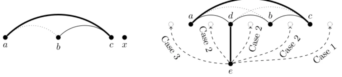
Proof. LetG,\sigma , and M be as described in the statement of the lemma (see

Fig-ure 4). The proof is by contradiction. Towards a contradiction let (a, b, c, x) be a quadruple of vertices satisfying all six conditions of the lemma. Fix now vertex x. Among all such quadruples with fixedx, let (a, b, c, x) be such thatais leftmost in\sigma ; that is, for any other such quadruple (a\prime , b\prime , c\prime , x) we havea\leq \sigma a\prime . Since\sigma is an LDFS

ordering, it follows from conditions 1 and 2 and Definitions 2.4 and 2.5 that there is a vertexdsuch thata <\sigma d <\sigma b,\{ d, b\} \in E, and\{ d, c\} \in /E. Since\{ d, c\} \in /E and\sigma is

umbrella-free, it follows that\{ a, d\} \in E. Observe thatdis matched inM as otherwise conditions 5 and 6 would be violated. Thus, there is a vertexe\in V with\{ e, d\} \in M. Now we distinguish three cases with respect to the position ofein the ordering\sigma .

Case 1: \bfitc <\bfitsigma \bfite . In this case we have thata <\sigma c <\sigma e,\{ d, e\} \in E, and\{ d, c\} \in /

E. Thus, since\sigma is umbrella-free, it follows that\{ c, e\} \in E. However, in this case for the matchingM\prime = (M \setminus \{ \{ a, c\} ,\{ d, e\} \} )\cup \{ \{ e, c\} ,\{ a, d\} \} we invoke Observation 2.8

a _b c x a d b c e Case 1 Case 2 Case 2 Case 2 Case 3

Fig. 4.Bold lines indicate matched edges; dotted lines indicate a nonedge. Left: Situation for

invoking Lemma 2.11displaying conditions 1to3wherec\not =x. Right: The case distinction in the

proof of Lemma 2.11over the position ofein the order.

withvi=eto obtainf(M\prime )< f(M), a contradiction.

Case 2: \bfita <\bfitsigma \bfite <\bfitsigma \bfitc . If\{ a, e\} \in E, then there exists the length-three

alternat-ing path (a, e, d, b) fromatobwithinG\sigma (x), which is a contradiction to condition 4.

Thus, \{ a, e\} \in / E. Furthermore, \{ c, e\} \in E, since\sigma is umbrella-free and\{ a, c\} \in E. Hence, for the matching M\prime = (M \setminus \{ \{ a, c\} ,\{ d, e\} \} )\cup \{ \{ e, c\} ,\{ a, d\} \} we invoke Ob-servation 2.8 withvi=cto obtainf(M\prime )< f(M), a contradiction.

Case 3: \bfite <\bfitsigma \bfita . In this case it follows similarly to Case 2 that\{ a, e\} \in / E(proof

by contradiction due to condition 4). Furthermore, observe that \{ e, d\} ,\{ a, d\} \in E

and \{ e, d\} \in M. Thus the triple (e, a, d) satisfies conditions 1 to 3. Furthermore,

if there exists an odd-length alternating path from e to a within G\sigma (x), then this

alternating path can be extended throughdto an odd-length alternating path from ato bwithinG\sigma (x), which is a contradiction to condition 4. Hence there is no

odd-length alternating path from eto a withinG\sigma (x). Similarly, odd-length alternating

paths frome(resp., froma) to a free vertexv withinG\sigma (x) are excluded as well due

to condition 5 (resp., due to condition 6). Thus the quadruple (e, a, d, x) satisfies the six conditions of the lemma and it holds thate <\sigma a, a contradiction to the choice of

the initial quadruple (a, b, c, x).

We are now ready to prove our central result.

Theorem 2.12. For any n-vertex and m-edge cocomparability graph G,

Algo-rithm 3 returns a maximum matchingM ofGin O(n+m)time.

Proof. LetG= (V, E) be a cocomparability graph, and let\sigma be an umbrella-free

LDFS ordering ofG. First we prove that Algorithm 3 runs inO(n+m) time. To this end, we denote with deg(v) the degree of a vertex v \in V. During the execution of the algorithm we maintain theunvisited vertices in a doubly linked listA(initially of sizen), according to their position in\sigma . Furthermore, we maintain for each vertexuits

unvisited neighborsin a doubly linked listNu(initially of size deg (u)), again according

to their position in\sigma . Once we have computed the ordering\sigma , the construction of the listA can be done inO(n) time. The construction of all lists Nu, whereu\in V, can

be done inO(n+m) time as follows. We initializeNu=\emptyset for everyu\in V. Then we

iterate for each vertexu\in V in the listA from left to right. For every such vertexu we scan (in an arbitrary order) through its neighborhood N(u) (note that Nu is at

this point still incomplete), and for eachv\in N(u) we append vertexuin the listNv.

Line 16 can be clearly executed inO(n) time. The rightmost unvisited vertexx in Line 18 can be found in O(1) time as the rightmost vertex in the listA. Oncex is detected in Line 18, x is removed from A also in O(1) time. Furthermore, x is removed from all lists Nu, where \{ x, u\} \in E, in O(deg (x)) time since x is always

the last element in the respective list. Moreover, Line 19 can be clearly executed in O(1) time. The if-condition of Line 20 can be checked inO(1) time by just checking whether the list Nx is empty. Similarly to Line 18, Line 21 can be executed in

O(deg (y)) time. Furthermore, each of Lines 22 to 24 can be clearly executed in O(1) time. Summarizing, the total running time of Algorithm 3 isO(n+\sum

u\in V deg (u)) =

O(n+m).

For the correctness part, the proof is done by contradiction. LetM be the match-ing returned by RMM(G, \sigma ). Assume towards a contradiction thatM is not a max-imum matching. For the rest of the proof, letM\prime denote a maximum matching that minimizesf(M\prime ) among all maximum matchings ofG. Letxbe the rightmost vertex in \sigma on which M differs from M\prime _{. Then x is matched in at least one of the two}

matchingsM andM\prime . Now we distinguish three cases with respect to the vertex that is matched withxinM andM\prime .

Case 1: \bfitx is matched in \bfitM \prime to some \bfity \in \bfitV but is free in \bfitM . Then

M and M\prime also differ at vertex y. Thus y <\sigma x, since x is the rightmost vertex

in which M and M\prime differ. Consider the iteration t of Algorithm 3 during which the algorithm visits x. If y is free inM, then this leads to a contradiction; indeed, otherwise Algorithm 3 would have matched x in iteration t as x has at least one unvisited neighbor, namelyy. Hence, the vertexy is matched inM with a vertexz at an earlier iteration t\prime < t. Then M differs fromM\prime also at vertex z. If z <\sigma x,

then Algorithm 3 visits xat an earlier iteration than z, which is a contradiction to the assumption on z. Hence x <\sigma z. This is a contradiction to the assumption that

xis the rightmost vertex in\sigma in whichM differs fromM\prime .

Case 2: \bfitx is matched in \bfitM to some vertex \bfity \in \bfitV but is free in \bfitM \prime .

If y is free in M\prime , then the matching M\prime \cup \{ \{ x, y\} \} is larger than M\prime , which is a contradiction to the maximality assumption on M\prime _{. Therefore, y is matched in M}\prime

to some vertex z \in V. Note that M and M\prime differ also on y and z. Thus, it follows by the choice of x that y <\sigma x and z <\sigma x. Consider now the matching

M\prime \prime := (M\prime \setminus \{ \{ y, z\} \} )\cup \{ \{ x, y\} \} , which is maximum since | M\prime \prime | =| M\prime | . However, invoking Observation 2.8 withvi=xyieldsf(M\prime \prime )< f(M\prime ), which is a contradiction

to the assumption on the minimality off(M\prime ).

Case 3: \{ \bfitx , \bfity \} \in \bfitM and \{ \bfitx , \bfitz \} \in \bfitM \prime with \bfitz \not = \bfity . Then M and M\prime

differ also ony and z. Thus, it follows by the choice of xthat y <\sigma xand z <\sigma x.

Consider the iterationtof Algorithm 3 during which the algorithm visitsx. Suppose that vertexzis matched inM with a vertexpat an earlier iterationt\prime < t. ThenM differs from M\prime also at vertex p. If p <\sigma x, then Algorithm 3 visits xat an earlier

iteration thanp, which is a contradiction to the assumption onp. Ifx <\sigma p, then we

have again a contradiction to the assumption that xis the rightmost vertex in\sigma in whichM differs fromM\prime . Thuszis unmatched inM at the iterationtof Algorithm 3 during which the algorithm visits x. Furthermore, z is also unvisited at iteration t since z <\sigma x. Now, if y <\sigma z, then Algorithm 3 would not match x to y at the

execution of Line 21, which is a contradiction. Hencez <\sigma y.

Suppose that y is free inM\prime . ThenM\prime \prime := (M\prime \setminus \{ \{ x, z\} \} )\cup \{ \{ x, y\} \} is another maximum matching. Invoking Observation 2.8 with vi = xyields f(M\prime \prime )< f(M\prime ),

a contradiction to the assumption on M\prime . Hence, y is matched in M\prime to some vertex w \in V with w <\sigma x by the choice of x. If \{ w, z\} \in E, then the

match-ing M\prime \prime := (M\prime \setminus \{ \{ x, z\} ,\{ w, y\} \} )\cup \{ \{ x, y\} ,\{ z, w\} \} is another maximum matching. Invoking Observation 2.8 withvi =xyields f(M\prime \prime )< f(M\prime ), which a contradiction

to the choice ofM\prime . Hence\{ z, w\} \in / E.

Suppose that withinG\sigma (x) (Definition 2.10) there exists an odd-length alternating

pathP0with respect toM\prime from wtoz. LetE0 be the edges in the pathP0. Then,

swapping inM\prime all edges on the pathP0(that is, replacing in M\prime the edgesM\prime \cap E0

with the edges E0\setminus M\prime ), removing \{ x, z\} and \{ w, y\} from M\prime , and adding \{ x, y\}

yields another maximum matching M\prime \prime . Recall that x is the rightmost vertex in whichM andM\prime differ. Thus, since the alternating pathP0 belongs to the induced

subgraph G\sigma (x), it follows from Observation 2.8 withvi =xthat f(M\prime \prime )< f(M\prime ),

a contradiction to the choice of M\prime . Thus, within G\sigma (x) there exists no odd-length

alternating path with respect toM\prime fromwto z.

Similarly, suppose that within G\sigma (x) there exists an odd-length alternating

pathP1with respect toM\prime fromw(resp., fromz) to a free vertexv. Then, swapping

inM\prime _{all edges on the pathP}

1, removing\{ x, z\} and\{ w, y\} fromM\prime , and adding\{ x, y\}

yields another maximum matchingM\prime \prime for which Observation 2.8 withvi=ximplies

f(M\prime \prime )< f(M\prime ), which is again a contradiction to the choice ofM\prime . Thus there exists withinG\sigma (x) no odd-length alternating path with respect toM\prime fromw(resp., fromz)

to a free vertexv.

Now suppose thatw <\sigma z. That is,w <\sigma z <\sigma y, where\{ w, y\} \in Eand\{ z, w\} \in /

E. Hence,\{ z, y\} \in Esince\sigma is umbrella-free. Thus, since\{ w, y\} \in M\prime , it follows that the quadruple (w, z, y, x) satisfies all six conditions in the statement of Lemma 2.11. This is a contradiction to Lemma 2.11, sinceM\prime is assumed to be a maximum matching ofGsuch thatf(M\prime ) is minimum among all maximum matchings.

Finally, suppose thatz <\sigma w. Recall thatM differs fromM\prime inw, since\{ y, w\} \in

M\prime and \{ x, y\} \in M. Thus, since x is the rightmost vertex in\sigma in which M differs fromM\prime , it follows thatw <\sigma x. That is,z <\sigma w <\sigma x, where\{ x, z\} \in Eand\{ z, w\} \in /

E. Hence,\{ w, x\} \in Esince\sigma is umbrella-free. Thus, since\{ x, z\} \in M\prime , it follows that the quadruple (z, w, x, x) satisfies all six conditions in the statement of Lemma 2.11. This is again a contradiction to Lemma 2.11, sinceM\prime _{is assumed to be a maximum}

matching ofGsuch thatf(M\prime ) is minimum among all maximum matchings. Summarizing, the matchingM returned by Algorithm 3 is a maximum matching.

3. Conclusion. We presented a thorough mathematical analysis of an efficient

and easy-to-implement linear-time greedy algorithm for computing maximum match-ings on cocomparability graphs. This contributes to a long list of polynomial-time algorithms for problems on cocomparability graphs. Notably, most of this previous work showed polynomial-time (typically far from linear) algorithms for problems that are NP-hard on general graphs, while we improved a problem solvable in polynomial time on general graphs to linear time on cocomparability graphs.

Apart from being of interest on its own, our result might also be useful in a more general approach towards deriving faster algorithms for computing maximum matchings in relevant special cases. The fundamental idea behind this, as described in the companion work [40], is as follows. First observe that, once a matching is given which haskfewer edges than an optimal one, then usingkiterated augmenting path computations (each taking linear time [18]), one can improve it to a maximum matching. If for a graph G we also have a vertex subset set X, | X| = k, such thatG - X is a cocomparability graph, then for constantkwe could get a linear-time algorithm for_Matching as follows: First, delete thek vertices fromG, then apply our linear-time algorithm, and then apply (as described above) at mostk iterations of augmenting path computations again with respect to the original graphG, starting with the maximum matching for the cocomparability graph. A drawback of this approach is that we do not even know how to compute in linear time a constant-factor approximation (which would be good enough) for the mentioned vertex deletion set

of size k. Hence, we consider it as an interesting challenge for future work to give a linear-time (constant-factor approximation) algorithm for computing a ``minimum-vertex-deletion-to-cocomparability"" set. Based on the above considerations, for now we only can state the following result.

Corollary 3.1. Matchingcan be solved in O(k\cdot (n+m)) time when given a

size-k vertex set subsetX such that deleting X from the given graph yields a

cocom-parability graph.

From a more general point of view, Corollary 3.1 is a contribution to the ``FPT in P"" program [21], heading for more efficient polynomial-time algorithms based on problem parameterizations (also cf. [1, 9, 16, 17]).

Acknowledgment. We are deeply grateful to two anonymous reviewers for their

very careful reading and their constructive feedback, which helped us significantly clarify and improve the presentation.

REFERENCES

[1] M. Bentert, T. Fluschnik, A. Nichterlein, and R. Niedermeier,Parameterized aspects of

triangle enumeration, in Proceedings of the 21st International Symposium on Fundamen-tals of Computation Theory (FCT '17), Lecture Notes in Comput. Sci. 10472, Springer, Berlin, 2017, pp. 96--110.

[2] A. Brandst\"adt, V. B. Le, and J. P. Spinrad,Graph Classes: A Survey, SIAM Monogr.

Dis-crete Math. Appl. 3, SIAM, Philadelphia, 1999, https://doi.org/10.1137/1.9780898719796.

[3] M. Chang, Algorithms for maximum matching and minimum fill-in on chordal bipartite

graphs, in Proceedings of the 7th International Symposium on Algorithms and Computa-tion (ISAAC '96), Lecture Notes in Comput. Sci. 1178, Springer, Berlin, 1996, pp. 146--155.

[4] S. R. Coorg and C. P. Rangan,Feedback vertex set on cocomparability graphs, Networks, 26

(1995), pp. 101--111.

[5] D. Corneil and P. Kamula,Extensions of permutation and interval graphs, in Proceedings

of the 18th Southeastern Conference on Combinatorics, Graph Theory and Computing, 1987, pp. 267--275.

[6] D. G. Corneil, B. Dalton, and M. Habib,LDFS-based certifying algorithm for the minimum

path cover problem on cocomparability graphs, SIAM J. Comput., 42 (2013), pp. 792--807, https://doi.org/10.1137/11083856X.

[7] D. G. Corneil, J. Dusart, M. Habib, and E. K\"ohler,On the power of graph searching for

cocomparability graphs, SIAM J. Discrete Math., 30 (2016), pp. 569--591, https://doi.org/ 10.1137/15M1012396.

[8] D. G. Corneil and R. M. Krueger, A unified view of graph searching, SIAM J. Discrete

Math., 22 (2008), pp. 1259--1276, https://doi.org/10.1137/050623498.

[9] D. Coudert, G. Ducoffe, and A. Popa,Fully polynomial FPT algorithms for some classes of

bounded clique-width graphs, in Proceedings of the 29th Annual ACM--SIAM Symposium on Discrete Algorithms (SODA '18), ACM, New York, SIAM, Philadelphia, 2018, pp. 2765--2784, https://doi.org/10.1137/1.9781611975031.176.

[10] E. Dahlhaus and M. Karpinski,Matching and multidimensional matching in chordal and

strongly chordal graphs, Discrete Appl. Math., 84 (1998), pp. 79--91.

[11] J. S. Deogun and G. Steiner, Polynomial algorithms for Hamiltonian cycle in

cocom-parability graphs, SIAM J. Comput., 23 (1994), pp. 520--552, https://doi.org/10.1137/ S0097539791200375.

[12] F. F. Dragan,On greedy matching ordering and greedy matchable graphs, in Proceedings of

the 23rd International Workshop Graph-Theoretic Concepts in Computer Science (WG 1997), Lecture Notes in Comput. Sci. 1335, Springer, Berlin, 1997, pp. 184--198.

[13] R. Duan and S. Pettie,Linear-time approximation for maximum weight matching, J. ACM,

61 (2014), 1.

[14] J. Dusart and M. Habib,A new LBFS-based algorithm for cocomparability graph recognition,

Discrete Appl. Math., 216 (2017), pp. 149--161.

[15] J. Dusart, M. Habib, and D. G. Corneil,Maximal Cliques Structure for Cocomparability

Graphs and Applications, preprint, https://arxiv.org/abs/1611.02002, 2016.

[16] T. Fluschnik, C. Komusiewicz, G. B. Mertzios, A. Nichterlein, R. Niedermeier, and

N. Talmon,When can graph hyperbolicity be computed in linear time?, in Proceedings of

the 15th International Workshop on Algorithms and Data Structures (WADS '17), Lecture Notes in Comput. Sci. 10389, Springer, Berlin, 2017, pp. 397--408; Algorithmica, to appear, https://doi.org/10.1007/s00453-018-0522-6.

[17] F. V. Fomin, D. Lokshtanov, S. Saurabh, M. Pilipczuk, and M. Wrochna, Fully

polynomial-time parameterized computations for graphs and matrices of low treewidth, ACM Trans. Algorithms, 14 (2018), 34.

[18] H. N. Gabow and R. E. Tarjan,A linear-time algorithm for a special case of disjoint set

union, J. Comput. System Sci., 30 (1985), pp. 209--221.

[19] F. Gardi,Efficient algorithms for disjoint matchings among intervals and related problems, in

Proceedings of the 4th International Conference on Discrete Mathematics and Theoretical Computer Science (DMTCS '03), Lecture Notes in Comput. Sci. 2731, Springer, Berlin, 2003, pp. 168--180.

[20] A. C. Giannopoulou and G. B. Mertzios,New geometric representations and domination

problems on tolerance and multitolerance graphs, SIAM J. Discrete Math., 30 (2016), pp. 1685--1725, https://doi.org/10.1137/15M1039468.

[21] A. C. Giannopoulou, G. B. Mertzios, and R. Niedermeier, Polynomial fixed-parameter

algorithms: A case study for longest path on interval graphs, Theoret. Comput. Sci., 689 (2017), pp. 67--95.

[22] A. V. Goldberg and A. V. Karzanov, Maximum skew-symmetric flows and matchings,

Math. Program., 100 (2004), pp. 537--568.

[23] M. C. Golumbic, Algorithmic Graph Theory and Perfect Graphs, 2nd ed., Ann. Discrete

Math. 57, North--Holland, Amsterdam, 2004.

[24] J. E. Hopcroft and R. M. Karp,An n5/2 _{algorithm for maximum matchings in bipartite}

graphs, SIAM J. Comput., 2 (1973), pp. 225--231, https://doi.org/10.1137/0202019.

[25] A. Ilic,Efficient algorithm for the vertex connectivity of trapezoid graphs, Inform. Process.

Lett., 113 (2013), pp. 398--404.

[26] E. K\"ohler and L. Mouatadid,Linear time LexDFS on cocomparability graphs, in Proceedings

of the 14th Scandinavian Symposium and Workshops on Algorithm Theory (SWAT 14), Lecture Notes in Comput. Sci. 8503, Springer, Berlin, 2014, pp. 319--330.

[27] D. Kratsch and L. Stewart,Domination on cocomparability graphs, SIAM J. Discrete Math.,

6 (1993), pp. 400--417, https://doi.org/10.1137/0406032.

[28] T. Krawczyk and B. Walczak, Extending partial representations of trapezoid graphs, in

Proceedings of the 43rd International Workshop on Graph-Theoretic Concepts in Computer Science (WG), Lecture Notes in Comput. Sci. 10520, Springer, Berlin, 2017, pp. 358--371.

[29] Y. D. Liang and M. Chang, Minimum feedback vertex sets in cocomparability graphs and

convex bipartite graphs, Acta Informatica, 34 (1997), pp. 337--346.

[30] Y. D. Liang and C. Rhee, Finding a maximum matching in a circular-arc graph, Inform.

Process. Lett., 45 (1993), pp. 185--190.

[31] L. Lov\'asz and M. D. Plummer,Matching Theory, Ann. Discrete Math. 29, North--Holland,

Amsterdam, 1986.

[32] T. Ma and J. P. Spinrad,On the2-chain subgraph cover and related problems, J. Algorithms,

17 (1994), pp. 251--268.

[33] A. Madry,Navigating central path with electrical flows: From flows to matchings, and back,

in Proceedings of the 54th Annual IEEE Symposium on Foundations of Computer Science (FOCS '13), IEEE, Washington, DC, 2013, pp. 253--262.

[34] R. M. McConnell and J. Spinrad,Linear-time modular decomposition and efficient

transi-tive orientation of comparability graphs, in Proceedings of the Tenth Annual ACM--SIAM Symposium on Discrete Algorithms (SODA), ACM, New York, SIAM, Philadelphia, 1994, pp. 536--545.

[35] G. B. Mertzios,The recognition of triangle graphs, Theoret. Comput. Sci., 438 (2012), pp.

34--47.

[36] G. B. Mertzios,An intersection model for multitolerance graphs: Efficient algorithms and

hierarchy, Algorithmica, 69 (2014), pp. 540--581.

[37] G. B. Mertzios, The recognition of simple-triangle graphs and of linear-interval orders is

polynomial, SIAM J. Discrete Math., 29 (2015), pp. 1150--1185, https://doi.org/10.1137/ 140963108.

[38] G. B. Mertzios and D. G. Corneil,Vertex splitting and the recognition of trapezoid graphs,

Discrete Appl. Math., 159 (2011), pp. 1131--1147.

[39] G. B. Mertzios and D. G. Corneil, A simple polynomial algorithm for the longest path problem on cocomparability graphs, SIAM J. Discrete Math., 26 (2012), pp. 940--963, https: //doi.org/10.1137/100793529.

[40] G. B. Mertzios, A. Nichterlein, and R. Niedermeier,The power of linear-time data

re-duction for maximum matching, in Proceedings of the 42nd International Symposium on Mathematical Foundations of Computer Science (MFCS), 2017, 46.

[41] G. B. Mertzios, I. Sau, and S. Zaks,A new intersection model and improved algorithms for

tolerance graphs, SIAM J. Discrete Math., 23 (2009), pp. 1800--1813, https://doi.org/10. 1137/09075994X.

[42] G. B. Mertzios, I. Sau, and S. Zaks, The recognition of tolerance and bounded tolerance

graphs, SIAM J. Comput., 40 (2011), pp. 1234--1257, https://doi.org/10.1137/090780328.

[43] G. B. Mertzios and S. Zaks,On the intersection of tolerance and cocomparability graphs,

Discrete Appl. Math., 199 (2016), pp. 46--88.

[44] S. Micali and V. V. Vazirani,AnO(\sqrt{}

| V| | E| )algorithm for finding maximum matching in

general graphs, in Proceedings of the 21st Annual IEEE Symposium on Foundations of Computer Science (FOCS '80), IEEE, Washington, DC, 1980, pp. 17--27.

[45] A. Moitra and R. C. Johnson, A parallel algorithm for maximum matching on interval

graphs, in Proceedings of the International Conference on Parallel Processing (ICPP '89), Pennsylvania State University Press, University Park, PA, 1989, pp. 114--120.

[46] M. Mucha and P. Sankowski,Maximum matchings via Gaussian elimination, in Proceedings

of the 45th Annual IEEE Symposium on Foundations of Computer Science (FOCS '04), IEEE, Washington, DC, 2004, pp. 248--255.

[47] M. Mucha and P. Sankowski,Maximum matchings in planar graphs via Gaussian

elimina-tion, Algorithmica, 45 (2006), pp. 3--20.

[48] S. Olariu,An optimal greedy heuristic to color interval graphs, Inform. Process. Lett., 37

(1991), pp. 21--25.

[49] P. Sankowski,Maximum weight bipartite matching in matrix multiplication time, Theoret.

Comput. Sci., 410 (2009), pp. 4480--4488.

[50] J. P. Spinrad,Efficient Graph Representations, Fields Inst. Monogr. 19, AMS, Providence,

RI, 2003.

[51] G. Steiner and J. S. Yeomans,A linear time algorithm for maximum matchings in convex

bipartite graphs, Comput. Math. Appl., 31 (1996), pp. 91--96.

[52] A. Takaoka, Graph isomorphism completeness for trapezoid graphs, IEICE Trans., 98-A

(2015), pp. 1838--1840.

[53] A. Takaoka,A Recognition Algorithm for Simple-Triangle Graphs, preprint, https://arxiv.

org/abs/1710.06559, 2017.

[54] A. Takaoka,Recognizing simple-triangle graphs by restricted 2-chain subgraph cover, in

Pro-ceedings of the 11th International Conference and Workshops on Algorithms and Compu-tation (WALCOM), 2017, pp. 177--189.

[55] M. Yu and C. Yang,An O(n)time algorithm for maximum matching on cographs, Inform.

Process. Lett., 47 (1993), pp. 89--93.

[56] R. Yuster,Maximum matching in regular and almost regular graphs, Algorithmica, 66 (2013),

pp. 87--92.