Instrumental Variable Estimation of Treatment Effects for
Duration Outcomes
Govert E. Bijwaard
∗Econometric Institute
Erasmus University Rotterdam
Econometric Institute Report EI 2007-20
∗Erasmus University Econometric Institute, P.O. Box 1738, 3000 DR Rotterdam, The Netherlands; Phone:
(+31) 10 40 81424; Fax: (+31) 10 40 89162; E-mail:[email protected]. This research is financially supported by the Netherlands Organization for Scientific Research (NWO) no. 451-04-011. I am very grateful to Geert Ridder for his comments and suggestions. I also benefited from the comments of participants at the 2003 Extending the Tinbergen Heritage conference in Rotterdam, at the 2003 ESEM Meeting, at the 14th
EC2
conference and, at the Econometric Evaluation of Public Policies : Methods and Applications in Paris 2005. I thank Steve Woodbury and the W. E. Upjohn Institute for making the data available to me.
Instrumental Variable Estimation of Treatment Effects
for Duration Outcomes
Abstract
In this article we propose and implement an instrumental variable estimation proce-dure to obtain treatment effects on duration outcomes. The method can handle the typical complications that arise with duration data of time-varying treatment and censoring. The treatment effect we define is in terms of shifting the quantiles of the outcome distribution based on the Generalized Accelerated Failure Time (GAFT) model. The GAFT model encompasses two competing approaches to duration data; the (Mixed) Proportional Haz-ard (MPH) model and the Accelerated Failure Time (AFT) model. We discuss the large sample properties of the proposed Instrumental Variable Linear Rank (IVLR), and show how we can, with one additional step, improve upon its efficiency. We discuss the em-pirical implementation of the estimator and apply it to the Illinois re-employment bonus experiment.
JEL classification:C21, C41, J64.
1
Introduction
In recent years, social experiments have gained popularity as a method for evaluating social and labor market programs (see e.g. Meyer (1995), Heckman et al. (1999) and Angrist and Krueger (1999)). In experiments the assignment of individuals to the treatment can be manipulated. If assignment is random, the average impact of the treatment can be estimated. However, a randomized assignment may be compromised, if the individuals can refuse to participate, either by dropping out, if they are to receive the treatment, or by obtaining the treatment, if they are in the control group. If this non–compliance to the assigned treatment is correlated with the outcome variable, i.e. is selective, then the difference of the average outcomes is a biased estimate of the average effect of the treatment.
Most of the evaluation literature has focused on static treatments, i.e. treatment that is administered at a particular point in time or in a particular time interval. If the outcome is a duration the treatment or its effect can be dynamic,i.e.it can be switched on and off over time. A further complication with duration data is that the durations are often censored. Examples of evaluation studies based on duration outcomes are Ham and LaLonde (1996), Meyer (1995), Van den Berg et al. (2004), Ashenfelter et al. (2005) and Bijwaard and Ridder (2005). These studies show that simple comparisons between average durations in the various treatment regimes are confounded by dynamic selection. We specify a causal model for duration outcomes that can handle censoring and time-varying treatments. The treatment effect in this model is defined in terms of shifting the quantiles of the survival rate.
Two competing approaches to the estimation of the effect of a, possible time–varying, covari-ate on survival has been the (Mixed) Proportional Hazard (MPH) model (for a recent survey see Van den Berg (2001)) and the Accelerated Failure Time (AFT) model (see a.o. Kalbfleisch and Prentice (2002), Br¨ann¨as (1992), and Klein and Moeschberger (1997)). In the Mixed Pro-portional Hazards (MPH) model the hazard is written as the product of the baseline hazard, a non-negative regression function, and a non-negative random variable that represents the covariates that are omitted from the regression function. Ridder (1990) introduced the Gener-alized Accelerated Failure Time (GAFT) model, a generalization of the AFT models that also includes the MPH model.
The GAFT model is based on transforming the duration and assuming some distribution for this transformed duration. The transformation is the integrated hazard of a PH model. The
AFT model is obtained by restricting the transformation but it does not restrict the distribution of the transformed duration, while the MPH model restricts the this distribution to a mixed of exponentials. The GAFT model is also related to the generalized regression model of Han (1987). The regression coefficients in a GAFT model can be interpreted in terms of the effect of regressing on the quantiles of the distribution of the transformed duration for the reference individual. In an AFT model the relation between the quantile of a individual with observed characteristics X and the quantile of the reference individual is the acceleration factor. In a GAFT this acceleration factor is multiplied by the ratio of the duration dependence at the two quantile durations. We use the GAFT model to construct a causal model for duration outcomes. Our approach to obtain the treatment effect in a duration model is related to rank es-timation procedures of Robins and Tsiatis (1991) and of Bijwaard and Ridder (2005). The procedure of Bijwaard and Ridder (2005) is based on a semi-parametric MPH and requires pre-liminary estimates of the baseline hazard. The procedure of Robins and Tsiatis (1991) is based on the strong version of the Accelerated Failure Time model. Their model imposes a strong non-interaction assumption. This implies that if two individuals have the identical observed durations and observed treatment histories then they would have had identical durations had treatment always been withheld.
We propose an instrumental variable procedure for duration models that does neither impose the non-interaction assumption nor requires full compliance in the control group. It enables us to estimate the treatment effect in terms of changes in the quantiles. This is accomplished by using a GAFT model that transforms the duration such that for the true, population, parameter the transformed duration is independent of the instrument. Thus, for a binary instrument, R, the proportion of the people withR= 1 remains the same over the survivors on the transformed duration time. This implies that the rank test statistic for the instrument on the relevant time scale, i.e. the transformed duration time scale, should go to zero. The inverse of this rank test,or a weighted version, provides the estimation procedure we call the Instrumental Variable Linear Rank (IVLR) estimation.
The existence of an endogenous treatment implies (possible) dependence between the trans-formed duration and the censoring time. This implies that the IVLR estimator, which exploits the independence between the transformed durations and the instruments, may give biased re-sults. However, with a small adjustment we can still apply the IVLR approach, based upon the assumption that the (potential) censoring time is known at the start of the study. For example,
in our empirical data, we only observed the unemployed while receiving UI benefits. In these data the potential censoring time for all individuals is at 26 weeks, the maximum duration of receiving UI benefits. With known (potential) censoring time we can modify the GAFT trans-formation by introducing additional censoring such that this modified transtrans-formation and the instruments become independent for the uncensored observations. Then, the IVLR estimator on this modified transformation leads to consistent estimators.
The IVLR estimation is based on a vector of mean restrictions on weight functions of the covariates, instrument and the transformed durations. Thus the IVLR is also related to GMM estimation. In GMM estimation it is feasible to get the most efficient, optimal, GMM estimator in just two steps. At the first step a GMM estimator is obtained using suboptimal, but feasible, weighting matrices. From this consistent estimator the optimal weighting matrices can be estimated consistently. With these estimated matrices we can obtain an efficient estimate of the parameters involved in just one additional step. A similar reasoning applies to the IVLR-estimator. At the first step we use feasible weighting functions to obtain consistent estimates of the parameters of the GAFT model. From these parameters we estimate the distribution of the transformed durations, which is needed to calculate the most efficient weighting functions. Then, in just one additional step the efficient IVLR estimator is obtained.
Our approach identifies the treatment effect in terms of the effect of the quantiles of the transformed duration. It is therefore not surprising that our approach is also related to quantile regression. Koenker and Geling (2001) and Koenker and Bilias (2001) use quantile survival regression to identify the treatment effect as the difference between the two marginal survival distributions of treated and untreated individuals. It is, however, unclear how these methods can handle time-varying treatment.
Various other papers consider methods for Instrumental Variable estimation for duration models that are related to the approach of this paper. We mentioned already the methods developed by Robins and Tsiatis (1991) and by Bijwaard and Ridder (2005). Recently the application of the timing-of-events approach, introduced by Abbring and van den Berg (2003) has emerged. This method identified the causal effect on the hazard rate in a MPH model. The important identifying assumption is that the time to the treatment randomly varies between the individuals. Thus, when the timing of the treatment follows a predescribed protocol, as is the case for the bonus data, the timing-of-events method cannot be used to obtain the treatment effect. Abbring and van den Berg (2005) show that for a binary time-invariant treatment the
(fixed) treatment effect on the hazard rate in an MPH model is identified. The treatment effect can then consistently be estimated based on the behaviour of very short durations. The practical use of this estimator is limited because very short durations are often ill-recorded. Chesher (2002) considers an MPH-type model with an endogenous continuous treatment as well as exogenous variables, a continuous instrument, and a latent variable relating the treatment and the instrument.
For our empirical application we use data from the Illinois unemployment bonus experi-ment. These data have been analysed before with increasing sophistication by Woodbury and Spiegelman (1987), Meyer (1996) and Bijwaard and Ridder (2005). In this experiment a group of individuals who became unemployed during four months in 1984 were divided at random in three groups of about equal size: two bonus groups and a control group. The unemployed in the claimant bonus group qualified for a cash bonus if they found a job within 11 weeks and would hold this job for at least four months. In the employer bonus group, the bonus was paid to their employer. The members of the two bonus groups were asked whether they were prepared to participate in the experiment. About 15% of the claimant bonus and 35% of the employer bonus groups refused participation. The reason for this refusal is unknown, and it is very likely that the decision to participate is related to the unemployment duration. This makes the indicator of being eligible for a bonus an endogenous treatment variable.
The outline of the article is as follows. Section 2 provides the definition of treatment effect in the Generalized Accelerated Failure Time model. We also discuss identification. Section 3 pro-vides the intuition behind the Instrumental Variable Linear Rank estimator that is introduced in Section 4. We prove the consistency and asymptotic normality of the estimator and discuss the efficiency and the practical implementation of the IVLR. In Section 5 we apply the IVLR estimator to estimate the treatment effect of a re-employment bonus based on the Illinois bonus experiment. We conclude with a summary of the proposed procedure and empirical results, and discuss avenues for further research.
2
Treatment effects in Duration Models
We consider the population of individuals flowing into unemployment, and the durations these individuals subsequently spend in unemployment. Each individual is either assigned to a pre-described treatment protocol or to a control group. Thus, we know for each individual when the treatment is turned on or off. We are interested in the causal effect of the treatment on the
unemployment duration.
It can rarely be defended that a study on unemployment durations includes all the relevant characteristics of the individuals looking for a job. For example, consider a study on the effect of a re-employment bonus on finding a job within a certain period. Because such a bonus increases the reward of leaving unemployment it gives an incentive to search more intensively and therefore it is expected to increase the re–employment hazard. However, the search intensity of the unemployed individuals is usually not observed.
Suppose that the unemployed have to choose at the start of their unemployment spell whether they want to be eligible for a bonus. If they choose to be eligible they have to fill in some forms, notify their new employer and provide a proof that they held that job for at least 4 months. Thus, joining the bonus program implies some administrative duties and cooperation with their new employer for the unemployed. This might refrain some individuals from joining (as we see in our application). It is very likely that the unobserved motivation to return to work has an impact on both the decision to be eligible for a bonus and the search intensity. This makes the indicator of joining the bonus program an endogenous variable. Without adjusting for this (self)-selection standard duration analysis give biased results of the effect of the bonus on unemployment duration.
A way of adjusting for an endogenous treatment is the conventional instrumental variable assumptions of instrument–error independence and an exclusion restriction. A familiar example of an instrumental variable is a randomly assigned treatment for a policy in which the actual treatment still depends on a decision by the agents (or on decisions made by those who execute the program). For instance, long–term unemployed can be randomly assigned to a training program, but for many programs they can still decide not to join, or the training manager can decide to withhold some training from some people. Then, the assignment indicator is an instrument for the actual indicator of training received.
Complications arise if the outcome variable of interest is a duration variable, like the un-employment duration. Models for duration data are usually non-linear. In general the value of the treatment variable may depend on information that accumulates during the evolution of the duration. The common approach to accommodate such time-varying variables is to relate them to the hazard rate or survival rate. Another reason not to consider the effect on the mean is that duration data are usually (right)-censored, due to a limited observation window. The hazard rate and survival rate are invariant to censoring. We shall define the treatment effect
in terms of a change in the quantiles of the distribution based on a Generalized Accelerated Failure Time Model.
2.1
The Generalized Accelerated Failure Time Model
The key variables in duration analysis are the duration till the next event,T, and the indicator of censoring,δ. The observed durations may be right–censored, i.e. we observe ˜T = min(T, C) with
C the censoring time. The possible time–varying treatment indicators are given by the vector
Di(t) whereirefers to a member of the population. The path of the treatment is predetermined.
Thus D(t) ={D(s); 0≤s≤t} does not depend on future, after t events.
Two competing approaches for the analysis of duration data has been the (Mixed) Propor-tional Hazard (MPH) model and the Accelerated Failure Time (AFT) model. The MPH model assumes that the hazard, the instantaneous probability of an event at durationt, given that no event occurred before t can be written as
λ(t|D(t), V) =vλ0(s;α)eγD(t)
where λ0(t) represents the baseline hazard, that is, the duration dependence of the hazard
common to all individuals. The treatment affect, eγ′D(s)
, and the unobserved heterogeneity ,V, enter the hazard proportionally. The integrated hazard, Λv(t) =
Rt
0 λ(s|D(s), V)ds =
vRt
0λ0(s;α)eγD(s)ds is unit exponentially distributed, E(1) and therefore the MPH model is
also equivalent to Z t 0 λ0(s;α)eγD(s)ds∼ E (1) V (1)
Thus the distribution of Λ(t) =Rt
0 λ0(s;α)e
γ′D(s)
ds is a mixture of exponential distributions. The AFT model assumes that the survival function of an individual with covariate pathD(t) is related to the survival function of the untreated individual, the individual with D(t) = 0, by
S t|D(t)
=S0
Z t
0
eγ′D(s)ds
with S0(·) is the survival function of the untreated individual. Let T0 be the duration of an
untreated individual. If the treatment is time-invariant then an AFT model implies that the distribution of TD, the duration of an individual with treatment D, and the distribution of
e−γ′D
T0 are the same. Thus, the treatment D accelerates, γ < 0, or decelerates, γ > 0 the
duration. This is equivalent with a linear regression model for the log-duration ln(T) = −γ′D+ǫ
where ǫ is a random variable with same distribution as ln(T0).
A class of duration models that generalizes the AFT models in such a way that it also in-cludes the MPH models is the Generalized Accelerated Failure Time (GAFT) model, introduced by Ridder (1990). The GAFT model is not specified by the distribution of the log-duration. Instead, we transform the duration, and assume that this transformed duration has some distri-bution. The transformation of the duration is related to the integrated hazard in a PH-model. The GAFT model is related to the generalized regression model proposed by Han (1987).
The GAFT model assumes that the relation between the duration T and the treatment is specified as
Z T
0
λ(s;α)eψ(s,D(s),γ)ds=U =h T, D(T), θ
(2) where λ(t;α) is a non–negative function on [0,∞) and ψ(t, D(t), γ) is the treatment function with treatment coefficient (vector)γ andθ= (α′, γ′)′. For the true population parameter-vector θ0 we have U0 =h T, D(T), θ0
. We assume that the treatment is a binary variable that only changes at predescribed durations and that the treatment effect may change over the duration. Then a flexible functional form forψ is
ψ(t, D(t), γ) =
J
X
j=0
γj·Dj·Ij(t) (3)
where Ij(t) =I(tj < t≤tj+1) with t0 = 0 andtJ+1 =∞.
A flexible functional form for λ is the piecewise constant function. The GAFT model is characterized by these functions and by the distribution of the non–negative random variable
U0. We denote the survivor function ofU0 by G0(u), which does not depend on the treatment,
and its hazard function byκ0(u). We assume that the distribution ofU0is absolutely continuous.
The semi–parametric estimators considered in this article avoid assumptions on the distribution of U0.
As mentioned, the GAFT model contains as special cases the AFT, the PH and the MPH models. The AFT model restricts the transformation to λ(t;α)≡1, but leaves the distribution of U0 unrestricted (with the exception of that U0 should be non–negative, see e.g. Cox and
Oakes (1984)). The (M)PH model restricts the distribution ofU0, but leaves the λunrestricted
(non–negative). The distribution ofU0 is an unit exponential distribution (PH) or a mixture of
exponential distributions (MPH). A convenient assumption is that the unobserved heterogeneity has a gamma distribution with variance σ2. Then, U
0 has a Burr distribution with density
g0(u) = (1 +uσ2)−1−1/σ
2
2.2
Counterfactual analysis
We model the causal effect of the treatment on the unemployment duration using the potential-outcome framework, as formulated by Holland (1986) for static interventions, and extended by Robins (1986) to time-varying interventions.
Equation (2) implicitly defines the outcome, i.e. duration, distributions for the treatment and control groups. We indicate these regimes by the subscripts (1) and (0), respectively. The outcome distributions for the two regimes forT∗
(1), T(0)∗ are given by U∗ (0) = Z T(0)∗ 0 λ(s;α0)ds (4) U∗ (1) = Z T(1)∗ 0 λ(s;α0)eψ(s,1;γ0)ds (5)
The fundamental assumption that assures identification is that U∗
(0) and U(1)∗ have the same
distribution. They may be dependent, but the joint distribution is only identified in special cases and not of particular interest. A special case is that U∗
(1) ≡ U(0)∗ . In that case there is a
deterministic relation between the outcomes in the two regimes and,
Z T(0)∗ 0 λ(s;α0)ds = Z T(1)∗ 0 λ(s;α0)eψ(s,1;γ0)ds (6)
This model corresponds, but is not identical to the Rank Preserving Structural Failure Time (RPSFT) model of Robins and Tsiatis (1991). In the RPSFT model T∗
(0)i is the potential
duration of individual i, if she/he was never to receive the treatment. Thus, Robins and Tsiatis think of T∗
(0)i is the baseline duration for the never treated, as a pre–treatment characteristic
of the individual. An example of an RPSFT model is to assume that
T(0)∗ =
Z Ti
0
eψ(s,Di(s);γ0)ds (7)
The outcome model defined in (4) and (5) is also rank preserving. If we consider two individuals with potential outcomes T∗
(0)i, T(1)∗ i, i = 1,2, then T(0)1∗ > T(0)2∗ implies T(1)1∗ > T(1)2∗ and vice
versa. However, T∗ (0) 6= Z T(1)∗ 0 λ(s;α0)eψ(s,D(s);γ0)ds ψ(t,D(t);γ0)≡0 (8) and T∗
(0) cannot be interpreted as the latent baseline duration. An unattractive feature of the
RPSFT model is that it implies that individuals with the same outcome in the treatment regime have the same outcome in the no treatment regime, and the other way round. This equality of counterfactuals is a strong assumption.
Under the weaker assumption thatU∗
(0) and U(1)∗ have the same distribution, the relation in
(6) still holds but now for the quantiles of the outcome distribution. Thus we can interpret the treatment effect in terms of regressing on theU∗
(0) quantiles. Lettq(0) andtq(1) be the quantiles
of U∗ (0) and U(1)∗ then, G0 htq(1),1;θ0 = 1−q =G0 h tq(0),0;θ0 (9) Hence we obtain a relation between tq(1) andtq(0) that is defined implicitly by
Z tq(1) 0 λ(s;α0)eψ(s,1;γ0)ds = Z tq(0) 0 λ(s;α0)ds (10)
This implies that
dtq(1) dtq(0) =e−ψ tq(1),D(tq(1));γ0 × λ(tq(0);α0) λ(tq(1);α0) (11) In the MPH model we can interpretλ(t) as the baseline hazard, i.e. the factor in the proportional hazard that captures the (duration) time variation in the hazard function. Thus, in the MPH model the ratio in (11) can be interpreted as the ratio of baseline hazards.
Note that if the treatment is time-invariant and has a fixed coefficient,ψ(t, D, γ0) =γ0Dand
γ0 >0 then an AFT model would overestimate the treatment effect ifλ tq(0);α
< λ tq(1);α
and underestimate the treatment effect ifλ tq(0);α
> λ tq(1);α
. Hence failure to correct for variation in λ may bias the treatment coefficient.
It may be instructive to give an example. The hazard or re–employment rate of unemploy-ment durations often exhibits a spike just before the time that unemployunemploy-ment benefits are exhausted. This corresponds to a large increase in λ at that spike. Now let us assume that all unemployed who find a job receive a bonus data and that the bonus has a small impact on the job finding rate, so that tq(0) > tq(1). If tq(0) is in the spike while tq(1) is not, then the
left–hand side of (11) is greater than one and the AFT treatment effect at tq(1) is negative.
We conclude that if there is (substantial) variation in λ, the uncorrected treatment effects that can be directly estimated from the marginal outcome distributions are misleading.
2.3
Identification of the GAFT model
In the GAFT model with an exogenous treatment and a log–linear regression function, the model is characterized by the non–negative function λ(t;α) defined on [0,∞), the distribution of U0 and the regression parameter γ. Ridder (1990) has shown that if the covariates are time
constant, all observationally equivalent GAFT models, i.e. models that give the same condi-tional distribution of T given D, have regression parameters c1γ, integrated transformation
c2 Rt 0 λ0(s;α)ds c1 and U0 distributionG0 u c2 1/c1
for some constants c1, c2 >0. The
equiv-alent class follows from the fact that a GAFT model with time constant covariates can be expressed as a transformation model
ln Z T 0 λ0(s;α) ds d =−γD+ lnU,
and the constants c1, c2 correspond to addition of ec2 to and division by c1 of the left– and
right–hand sides.
With time–varying covariates, the set of observationally equivalent GAFT models is gener-ally smaller. In particular, the power transformation that gives an observationgener-ally equivalent model if the covariates are time constant, in general does not result in a GAFT model. As an example consider the GAFT model with time–varying regressors that differ between two groups. In groupI
D(t) =
(
1 if 0 ≤t≤1,
0 if t >1.
and in group II, D(t) = 0; t ≥ 0. Moreover λ0(t;α) = αtα−1. With time constant regressors
the parameter α is not identified. It can be shown that the observationally equivalent GAFT models have transformation c2tα and U0–distribution with c.d.f. Gu cu2
. Hence, with time– varying covariatesα is identified (and so isγ).
We conclude that identification depends on whether the covariates are time constant or time– varying. If the covariates are time constant we can identify the transformation h(T, D(T);θ) up to a power andγ up to scale (with the power and the scale being equal). Moreover, if we fix the power we can identify h(T, D(T);θ)c1 up to scale and the distribution ofU up to the same
scale parameter.
If the covariates are time–varying, we can, except in special cases, identify h(T, D(T);θ) and the distribution of U0 up to a common scale parameter. Because we leave the distribution
of U0 unspecified in our estimation method, we can not use restrictions on this distribution to
find the scale parameter. For that reason we normalize h(T, D(T);θ) by setting h(T,0;θ) = 1 for some t0 > 0. With time constant regressors we need the same normalisation, but in
addition we need to set one regression coefficient equal to one. Of course, we could choose a class of transformations that is not closed under the power transformation. This amounts to identification by functional form.
Finally, we need a condition on the sample paths of D in the population. If we rewrite (2) as Z T 0 elnλ(s;α)+ψ(s,D(s),γ)ds=U (12) we require that Pr lnλ(s;α) + lnψ(s, D(s), γ) = 0 = 0 (13)
where the probability is computed over the distribution of D as a random function of t and 0 is the zero function. In other words, lnλ is not collinear with D.
The identification issues in the GAFT model with endogenous treatment are the same as in the GAFT model with only exogenous variables, except that we need additional assumptions on the instrument. First, the instrument should only affect the duration through the treatment and not directly. Second, the value of the instrument should influence the value of the treatment in a non-trivial way, for example if both the instrument and the treatment are binary Pr(D= 1|R= 1)>0 and Pr(D= 0|R= 0) >0.
3
Instrumental Variable estimation for Duration data
If treatment choice is exogenous to the duration, standard techniques for the analysis of survival time data can be used to estimate the treatment coefficient. For example, we can use a Mixed Proportional Hazards model and estimate the treatment coefficient using (semi–parametric) Maximum Likelihood procedures, depending on the assumptions we make about the distribution of the unobserved heterogeneity, V, and the baseline hazard. If the model is correctly specified the MLE yields a consistent estimate. However, standard MLE will give biased estimation results if the treatment choice is endogenous.3.1
Common solutions to endogeneity in duration models
Consider, for example, a randomized trail with selective compliance to the assigned time-constant treatment. LetR= 0,1 be the random assignment andD= 0,1 the actual treatment. Since physical randomization implies that at time zero all attributes of the two groups are (in expectation) identical, a commonly used solution to the endogeneity problem, is to ignore the post–randomization compliance and rely on the analysis of the treatment assignment groups. This intention–to–treat analysis replaces the actual treatment D, by the treatment assignment
indicator R, in the estimation procedure. Further, if the model is correctly specified the esti-mated treatment coefficients will correspond to the overall effect that would be realized in the whole population, under the assumption that the compliance rate and the factors influencing compliance in the sample are identical to those that would occur in the whole population.
The major drawback of the intention–to–treat analysis is that the estimated effect is a mixture of the population effect and the effect on the compliance. Hence, if the treatment effectively raises the re–employment hazard, the intention–to–treat measure of this effect will diminish as non–compliance increases. Another disadvantage is that compliance is very likely to depend on the perceived effects of the treatment. If, for example, the unemployed know that being eligible for a re–employment bonus does not stigmatize them, they will be more prone to participate. Thus, when the pattern of compliance is a function of the perceived efficacy of the treatment the estimated intention–to–treat will not represent the overall effect of the treatment had it been adopted in the whole population.
Recently an alternative approach introduced by Abbring and van den Berg (2003) to the analysis of treatment effects in duration models has emerged. This timing-of-events method identified the causal effect on the hazard rate in a MPH model. The important identifying assumption is that the time to the treatment randomly varies between the individuals. Thus, when the timing of the treatment follows a predescribed protocol, as is the case for the bonus data, the timing-of-events method cannot be used to obtain the treatment effect.
Abbring and van den Berg (2005) show that for a binary time-invariant treatment the (fixed) treatment effect on the hazard rate in an MPH model is identified. In the MPH model the hazard rate is λ(t|D, V) =vλ0(s;α)eγ
′D
. The treatment effect γ can then consistently be estimated based on the behaviour of very short durations. The practical use of this estimator is limited because very short durations are often ill-recorded.
When a continuous instrument is available more general models of the treatment effect are identified. Chesher (2002) considers an MPH-type model with an endogenous continuous treat-ment D as well as exogenous variables X, a continuous instrument R, and a latent variable relating D and R. He demonstrates local identification of ratios of the derivatives of the in-dividual hazard rate with respect to D and R. Abbring and van den Berg (2005) prove that for an MPH model with perfect compliance in the control group and a binary treatment a time-varying treatment effect that possibly depends on X is identified.
procedures of Robins and Tsiatis (1991) and of Bijwaard and Ridder (2005). The procedure of Bijwaard and Ridder (2005) is based on a semi-parametric MPH and requires preliminary estimates of the baseline hazard. If there is full compliance in the control group these preliminary estimates can be obtained from the control sample. These estimates are substituted in the second stage estimation equation. Their 2 Stage Linear Rank Estimator (2SLR) is a device to reduce the computational burden by dividing the computation into two steps. This is appealing because in the 2SLR is the solution to a discontinuous estimating function. However, the first stage of the 2SLR estimator is based on a MPH model for the control group and can only be estimated if the individuals in that group do not have any possibility to get a treatment.
As discussed in Section 2.2, the procedure of Robins and Tsiatis (1991) is based on the strong version of the Accelerated Failure Time model. Their model imposes a strong non-interaction assumption. This implies that if two individuals have the identical observed durations and observed treatment histories then they would have had identical durations had treatment always been withheld.
We propose an Instrumental Variable (IV) procedure for duration models that does neither impose the non-interaction assumption nor requires full compliance in the control group. It enables us to estimate the treatment effect in terms of change in the quantiles, as defined in (11). This is accomplished by using a GAFT model that transforms the duration such that for the true, population, parameter the transformed duration is independent of the instrument.
The intuition behind the idea of transforming can be clarified by considering a simple example. Suppose we have data from an experiment on a treatment that may reduce unem-ployment duration. The assignment to treatment is random, but the compliance to the assigned treatment is selective. If the treatment has no impact on the re-employment hazard the prob-ability of observing an individual with assigned to treatment, R = 1, among the survivors at some unemployment duration t is equal to the treatment assignment probability at the start, Pr(R = 1). However, if the treatment has an effect, say positive, on the hazard this does not hold, because in that case the treated individuals will find a job faster. But the distributions of the counterfactual transformed durations U∗
(0) and U(1)∗ are both independent of the
treat-ment assigntreat-ment. Thus, on the transformed duration time-scale, using the true, population, parameters, U0 =h T, D(T), θ0
, in the GAFT model in (2) the proportion of the individuals in assignment group remains the same
Pr R= 1 |U0 ≥u
= Pr R= 1|T ≥0
In other words: the basic assumption underlying the IV estimator is that for the right GAFT model the distribution of the duration on the transformed time scale is independent of the instrument. This implies that the hazard of thepopulationtransformed duration is independent of the instrument. This independence only holds for the population parameters and therefore we can build an estimation procedure that exploits this conditional independence1. Independence
ofRand the hazard rate ofU0 implies (infinitely) many orthogonality restrictions. For instance,
if we assume independence of the hazard of U0 and R for u≤Cu, we can choose Cu so that it
corresponds to a specific quantile of the distribution ofU0. In section 4 we explore this moment
conditions that lead to the Instrumental Variable Linear Rank (IVLR) estimator.
3.2
Censoring and endogenous treatment in GAFT
A common feature of duration data is that some of the observations are censored. Assume the censoring time, C, is (potentially) known. For example, in the analysis of unemployment duration based on administrative data the duration is often only observed while the individual receives unemployment benefits. Usually, the maximum duration of receiving benefits is based on the labor market history of the individual and is recorded in the data. Then, the potential censoring time is known and the observed durations are ˜T = min(T, C) and ∆ = I(T ≤ C), where ∆ is one if T is observed.
One is tempted to define the censored transformed durations by the minimum of the transformed time till (potential) censoring and the transformed time till the event occurs,
˜
U(θ) = min h(T;θ), h(C;θ)
= h( ˜T;θ). However, with an endogenous treatment censoring makes some of the orthogonality conditions implied by the independence of the instrument and the transformed durations fail to hold. This can be illustrated by a simple example: Consider a fixed censoring time, all individuals have the same maximum duration of receiving benefits. Then for all individuals, irrespective of their treatment status, censoring occurs at time C. Suppose that treatment is time-invariant and has a constant treatment function, ψ(·) = γD. Finally, we assume that except for the treatment parameter, γ, all the parameters of λ are known. Hence
U0 =eγ0DΛ0(T) (15)
with Λ0(t) =
Rt
0λ(s, α0) ds. Hence, ifD= 0 censoring in the transformed time occurs at Λ0(C),
1
Here we only concentrate on a static binary instrument and a discrete, but possible time-varying according to a prescribed protocol, treatment. It is not difficult to extend the analysis to more, discrete, levels of both the instrument and the treatment and to have a sequential instruments.
but if D = 1 censoring occurs at eγ0Λ
0(C). Thus, if γ0 > 0, then all transformed durations in
the interval [Λ0(C), eγ0Λ0(C)] have D = 1, i.e belong to the treatment group (for γ0 < 0 the
boundaries are reversed). The hazard of U0 on this interval clearly depends on Dand hence on
R. The independence of the hazard ofU0andRonly holds up to the lower bound of the interval.
This implies that in the IVLR, which exploits this independence, the transformed durations that fall in the problematic interval have to be censored.
This can be generalized to a model with a time–varying treatment parameter and/or a time– varying treatment. Assume the piecewise constant structure for the treatment function in (3). This implies that for a duration in the interval (tk, tk+1], the treatment parameter is eγk. We
define the transformed censoring timeCU(θ) such that: (a)T ≥C impliesh(T;θ)≥CU(θ) and
(b) U0 and R are independent on the interval bounded above byCU(θ).
Note that we either observe T ≤ C and ∆ = 1, or T > C and ∆ = 0. The transformed censoring times (conditional on T, C > tk) that take all these considerations into account are
the sum of the transformed duration up to tk, h(tk;θ) and the censoring adjustment, i.e
CU(θ) = (RC 0 λ(s;α)P(s;γ) ds if T > C, RT 0 λ(s;α)P(s;γ) ds+ RC T λ(s;α)ds if T ≤C. (16)
where P(s;γ) =I(s ≥ tk)Qkj=0min(eγj,1). From the last term on the right–hand side of (16)
we see why we need to know C even for the uncensored observations. Otherwise we can not compute CU(θ) for these observations. We can estimate the treatment coefficient γ and the
parameters of λ from the following observed data ˜
U(θ) = min U(θ), CU(θ)
, ∆U(θ) =I U(θ)< CU(θ))
Now ˜U(θ0) is independent ofR for ∆U(θ0) = 1. Note that if, at least, one of the γ’s is different
from zero, we introduce extra censoring on the transformed durations, because then some units with ∆ = 1 have ∆U(θ) = 0.
4
Instrumental Variable Linear Rank Estimation
In this section we introduce the Instrumental Variable Linear Rank (IVLR) estimator of the GAFT model. The estimator is based on independence of the transformed durations
{U˜(θ0),∆U(θ0)} and R. The IVLR is motivated by (14) and is defined on the possibly
4.1
The IVLR estimator
For the population parameter vectorθ0 the hazard ofU0,κ0(u), is independent of the instrument
history up to h−01(u). This independence can be used to construct test statistics close to the linear rank test (see Prentice (1978)).2 The IVLR also exploits this independence and is the
estimation procedure derived from these rank tests.
The data is a random sample ˜Ti,∆i, Di(Ti), Ri, i= 1, . . . , N. For someθthis random sample
can be transformed to ˜Ui(θ),∆Ui (θ), D U i U˜i(θ)
, i= 1, . . . , N and this is the sample that is used
in the statistic Sn(θ;W) = n X i=1 ∆Ui (θ)nW U˜i(θ), Ri −W U˜i(θ) o (17) where W ( ˜Ui(θ) = Pn j=1I U˜j(θ)≥U˜i(θ) W U˜i(θ), Rj Pn j=1I U˜j(θ)≥U˜i(θ) ,
the average of the weight function evaluated at ˜Ui(θ) among the individuals still under
ob-servation at that (transformed) duration. Note that we used ∆U
i (θ) instead of ∆i to assure
independence of the instruments and the transformed durations for all uncensored observa-tions. The estimating equation that defines the IVLR estimator contains a left–continuous weight function W. The dimension of W is greater than or equal to the dimension of θ0. The
weight function may depend on ˜Ui(θ) and R. The variance of the IVLR estimator depends on
W and in section 4.2 we discuss the optimal choice of this function.
The interpretation ofSn(θ;W) is that it compares the weight function for a transformed
du-ration that ends at ˜Ui(θ) to the average of the weight functions at that transformed duration for
those individuals that are still under observation. The independence suggests that the difference of the weight function for individual i and the average weight function for the individuals still under observation is zero at the population parameter value θ0. In large samples this is correct
if we choose for instance W U˜i(θ), Ri
= Ri, because for θ =θ0 the transformed duration U0
is independent of Ri. For θ =θ0 the transformed durations U0i are identically distributed and
this implies that the rank statistic is zero in large samples for this choice of W.
The expression for the rank statistic simplifies if we order the observations by increasing trans-formed duration
˜
U(1)(θ)≤U˜(2)(θ)≤. . .≤U˜(N)(θ)
2
Hausman and Woutersen (2005) derive an instrumental variable estimator based on Kendall’s rank-correlation for the MPH model.
In the ordered transformed durations we obtain SN(θ, W) = N X i=1 ∆U(i)(θ) W U˜(i)(θ), R(i) − PN j=iW U˜(i)(θ), R(j) N +i−1 (18) The function SN is not continuous in θ. The points of discontinuity are values of θ that make
e.g. ˜U(k)(θ) and ˜U(k+1)(θ) equal. If ∆(k)(θ) = ∆(k+1)(θ) = 1, the discontinuity is
W U˜(k)(θ), R(k+1)
−W U˜(k)(θ), R(k)
N−k (19)
and this goes to 0 if N increases. Lemma 1 in the appendix shows that SN is asymptotically
equivalent to a linear (and hence continuous) function in θ.
Thus, the statistic Sn(θ;W) has mean zero at the population parameters and, therefore,
we base our estimator on the roots of Sn(θ;W) = 0. However, the estimating functions are
discontinuous, piecewise constant, functions of θ and a solution may not exist. For that reason we define the Instrumental Linear Rank estimator (IVLR) ˆθn(W) as the minimizer of the
quadratic form, i.e.
ˆ
θn(W) = inf{θ |Sn(θ;W)′Sn(θ;W)} (20)
If Sn(θ;W) were differentiable with respect to θ, then asymptotic normality can be proved
using Taylor series expansion in a neighborhood of θ0. Tsiatis (1990) showed that, if Sn(θ;W)
is not differentiable, as in the current problem, we can still use a linear approximation of
n−1/2S
n(θ;W). Using this approximation and the asymptotic normality of Sn(θ0;W), we can
show that√n(ˆθn(W)−θ0) is asymptotically normal. Let a(u;θ0) be the probability limit of the
average weight function (see assumption C6 in the appendix) evaluated atu,C0the transformed
censoring time for θ = θ0. The asymptotic properties of the IVLR estimator are summarized
in the following two theorems that use the following terms: Let di0(u) the derivative of the
hazard ofU(θ) w.r.t.θevaluated atθ =θ0 andV(u, θ) is the probability limit of the covariance
between di0(u) and W(u, Ri) at u. The assumptions are given in the appendix.
Theorem 1 (Consistency).
If assumptions C1 to C7 hold θˆn(W) converges in probability to θ0.
Proof:See the appendix.
If assumptions C1 to C9 hold and Q(W) has full rank, then √ n(ˆθn(W)−θ0) d →N 0, Q−1(W)Ω(W)Q′−1(W) (21) where Ω(W) = Z C0 0 a(u;θ0)κ0(u)du (22)
is the asymptotic variance of n−1/2S
n(θ0;W) and,
Q(W) =
Z C0
0
V(u, θ0)du (23)
the limiting covariance matrix of the processes W(u, Ri) and di0(u)/κ0(u).
Proof:See the appendix.
4.2
Efficiency of the IVLR estimator
Many different choices of the weight functions lead to consistent estimates of the parameters. By properly choosing the weight function the asymptotic variance of the IVLR can be minimized. Tsiatis (1990) has shown that for the AFT model with exogenous covariates weight functions proportional to uκ′
0(u)/κ0(u)X minimize the asymptotic variance of the estimated regression
parameters. In general the distribution of U0 is unknown. This distribution can, however,
con-sistently be estimated from the implied U from any IVLR with a weight function not involving these functionals.
The IVLR estimation is based on a vector of mean restrictions on weight functions of the co-variates, instrument and the transformed durations. GMM estimation is also based on moment conditions and in GMM estimation it is feasible to get the most efficient GMM estimator in just two steps. A similar reasoning applies to the IVLR-estimator. This justifies an adaptive con-struction of an efficient estimator. In the next section we address the practical implementation of an adaptive estimation procedure. First, we introduce the optimal weight function.
Theorem 3 (Optimal weight function in IVLR).
The weight–function that gives the smallest asymptotic variance for θˆn(W) is
Wopt(u, R))∝
di0(u)
κ0(u)
(24) The asymptotic covariance matrix of the optimal IVLR estimator reduces to
Ω−1(W
Proof of theorem 3. From 1 √n Sn(ϑ0;W) Sn(ϑ0;Wopt) d →N 0, Ω(W) Q(W)′ Q(W) Ω(Wopt)
follows that the matrix
Z =
Ω(W) Q(W)′
Q(W) Ω(Wopt)
is non–negative definite, the same is true for its inverse. In particular, the submatrices on the main diagonal of the inverse are non-negative definite. Hence the matrix
Q−1(W)Ω(W)Q′−1(W)
−Ω−1(W opt)
is a non-negative definite matrix.
Consider, for example, a GAFT model with a piecewise constant λ function,
λ(t, α) = J X j=0 eαjI(t j < t≤tj+1) (26)
with t0 = 0 and tL+1 = ∞ and the hazard on the last interval is normalized to 1, αL = 0.
Assume that the model has a constant treatment coefficient then by (24) the optimal weight functions are Wopt,αj = 1 +uκ ′ 0(u) κ0(u) ·RIj1(u) + (1−R)Ij0(u)+ (27) +R 1 +uκ0(u) f0(u|1, R)−f0(u) f0(u) +uf ′ 0(u|1, R)−f0(u) f0(u) Ij1(u) + + (1−R) 1 +uκ0(u) f0(u|0, R)−f0(u) f0(u) +uf ′ 0(u|0, R)−f0(u) f0(u) Ij0(u) Wopt,γ = R 1 +uκ ′ 0(u) κ0(u) + (28) +R 1 +uκ0(u) f0(u|1, R)−f0(u) f0(u) +uf ′ 0(u|1, R)−f0(u) f0(u)
where f0(u|D, R) is the density of U0 givenD and R,f0′(·) is the derivative of the density and
ID j (u) =I mj(D)< u≤mj+1(D) for mj(D) = Z tj 0 λ(s, α)eγDds
4.3
Estimation in practice
The statisticSn(θ;W) is a multi–dimensional step–function. Therefore, the standard Newton–
Raphson algorithm cannot be used to solve (20). One of the alternative methods for finding a zero of a non–differentiable function is the Powell-method. This method is a multidimensional version of the Brent algorithm, see Press et al. (1986, §10.5) and Powell (1964).
Related to the computation of optimal weight function is the estimation of the variance matrix for an arbitrary weight function.3 The difficulty in estimating the covariance matrix lies
in the calculation of the matrix Q(W) and not in the calculation of the variance matrix of the estimating equation. The latter can be consistently estimated by
ˆ Ω = 1 n n X i=1 ∆Ui (ˆθ)hW u, Ri −W(u,θˆ)ihW u, Ri −W(u,θˆ)i′ (29)
The optimal weight functions, the covariance matrix and the most efficient estimators are estimated in two steps. The first step consists of obtaining a consistent estimate of θ0 using a
weight function that does not depend on the distribution of U0. For the example of a GAFT
model with a piecewise constant λ and a time-invariant treatment coefficient, a choice for the weight functions are Ij(u) and R. The transformed durations for these parameter values are
estimates of the unobserved population transformed durations. The second step concerns the estimation of the unknown distribution of U0. Many different methods are available to get a
reasonable estimate of an unknown distribution. We shall notapply the commonly used kernel based method. Although kernel–smoothed hazard rate estimators have been developed and adjusted to deal with the boundary problems inherent to hazard rates these methods can be difficult to implement due to the choice of the bandwidth. It is also unclear how the boundary corrections can be incorporated in the kernel estimates of the derivative of the hazard. We therefore choose to use a series approximation of the distribution.
Suppose the distribution ofU0 can be approximated arbitrary well using orthonormal
poly-nomials. We base our approximation on Hermite polynomials using the exponential distribution as a weighting function: g0(u) = ae−au PL l=0b2l hXL l=0 blLl(u) i2 (30) 3
Robins and Tsiatis (1991) suggested to use a numerical derivative ofn−1
Sn(θ;W) that does not need an
estimate of the optimal W–function to get ˆQ(W). This numerical derivative is sensitive to the choice of the difference inθ. We found it hard to get stable results.
where Ll(u) = l X k=0 l k (−au)k k! (31)
are the Laguerre polynomials. The unknown parameters of this approximation are a and
b0, . . . , bL. If bl ≡ 0 for all l > 0 the distribution of U0 is exponential. Even for L as small
as three (30) allows for many different shapes ofκ0(u) and its derivative. Both can be derived
analytically given the estimates of the parameters. The parameter estimators can be obtained from standard maximum likelihood procedures on the observed ( ˜Ui(ˆθn(W)),∆i).
If a consistent but inefficient estimator ˆθn(W) of θ0 is available and we have estimated the
parameters of the polynomial approximation of the distribution ofU0 we can obtain an efficient
estimator ˆθopt in just one additional step. From the linearization of the estimating equations,
given in (43) in the appendix, we obtain an efficient estimator from ˆ
θopt = ˆθn(W)−Qˆ(W)−1Sn(ˆθn(W);Wopt)/n (32)
This procedure is related to obtaining an efficient GMM estimator in two steps from a consistent, but possible, inefficient GMM estimator. It also possible to obtain the efficient estimator directly from minimizing the quadratic form. However, this involves again the minimization of a multi– dimensional step function.
5
Application to the Illinois Re-employment Bonus
Ex-periment
Between mid–1984 and mid–1985, the Illinois Department of Employment Security conducted a controlled social experiment.4 This experiment provides the opportunity to explore, within a
controlled experimental setting, whether bonuses paid to Unemployment Insurance (UI) ben-eficiaries or their employers reduce the time spend in unemployment relative to a randomly selected control group. In the experiment, newly unemployed claimants were randomly divided into three groups: a Claimant Bonus Group, a Employer Bonus Group and, a control group. The members of both bonus groups were instructed that they (Claimant group) or their em-ployer (Emem-ployer group) would qualify for a cash bonus of $500 if they found a job (of at least 30 hours) within 11 weeks and, if they held that job for at least four months. Each newly
4
A complete description of the experiment and a summary of its results can be found in Woodbury and Spiegelman (1987).
unemployed individual who was randomly assigned to one of the two bonus groups had the possibility to refuse participation in the experiment.
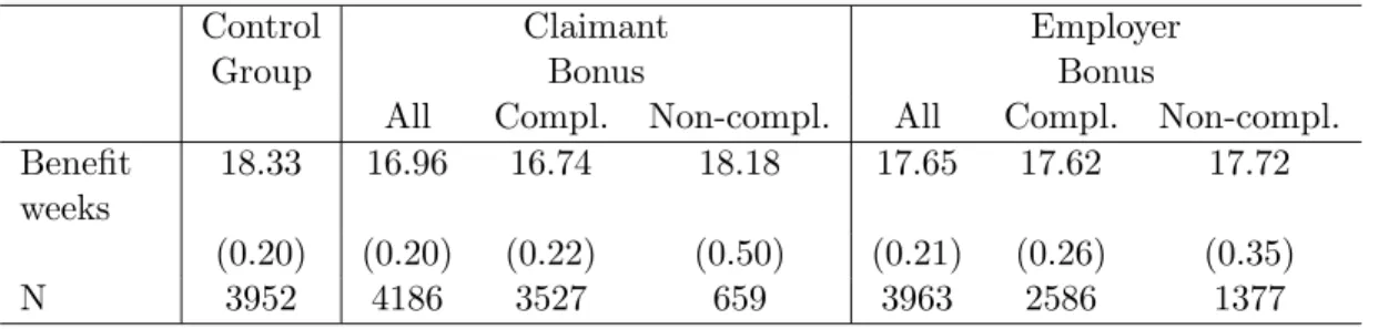
Woodbury and Spiegelman (1987) concluded from a direct comparison of the control group and the two bonus groups that the claimant bonus group had a significantly smaller average unemployment duration. The average unemployment duration was also smaller for the employer bonus group, but the difference was not significantly different from zero. These results are confirmed in table 1. Note that the response variable is insured weeks of unemployment. Because UI benefits end after 26 weeks, all unemployment durations are censored at 26 weeks. In table 1 no allowance is made for censoring. In the table we distinguish between compliers, those who agreed to be eligible for a bonus if assigned to a bonus group, and non-compliers. We see that the claimant bonus only affects the compliers and that the average unemployment duration of the non-compliers and the control group are almost equal.
Table 1: Average unemployment durations:control group and (non-)compliers.
Control Claimant Employer
Group Bonus Bonus
All Compl. Non-compl. All Compl. Non-compl. Benefit
weeks
18.33 16.96 16.74 18.18 17.65 17.62 17.72
(0.20) (0.20) (0.22) (0.50) (0.21) (0.26) (0.35)
N 3952 4186 3527 659 3963 2586 1377
standard error of average in brackets.
About 15% of Claimant group and 35% of the employer group declined participation. The reason for this refusal is unknown. Bijwaard and Ridder (2005) showed that the participation rate is significantly related to some observed characteristics of the individuals that also influence that re–employment hazard. Hence, we cannot exclude the possibility of unmeasured variables that affect both the compliance decision and the re–employment hazard. Meyer (1996) ana-lyzed the same data with a PH model with a piecewise constant baseline hazard. He used the randomization indicator instead of the actual bonus-group agreement indicator as an explana-tory variable. Thus he used the ITT estimator. He found a significantly positive effect of the claimant bonus. However, as shown by Bijwaard and Ridder (2005), the ITT has a downward bias.
We calculate the IVLR estimate of the effect of the claimant and employer bonus on the unemployment duration in a GAFT model and compare these estimates with the IVLR esti-mates of an AFT model, with ITT estiesti-mates in an MPH model and the ML estiesti-mates of an
MPH model that ignores the endogeneity of the decision to participate in the bonus group. We consider the two interventions separately: thus Claimant Bonus group versus Control group and Employer Bonus group versus Control.
We consider two alternative specifications for the treatment function of the bonus on unem-ployment duration: (i) constant treatment function and, (ii) a change in the treatment function after 10 weeks, in line with the end of the eligibility period of the bonuses. Thus, the implied transformed durations are
U(θ) =
Z T
0
λ(s;α)e(γ1I1(s)+γ2I2(s))Dds (33)
with I1(t) =I(0≤t <11) andI2(t) is its complement. We employ two different specifications
for λ(t;α0): (i) AFT model, i.e. λ(t;α0)≡1; and (ii) GAFT model with a piecewise constant
λ on six intervals 0–2, 2–4, 4–6, 6–10, 10–25 and 25 and beyond.
For identification we need to set one of the parameters of the piecewise constant λ equal to one (or the log equal to zero). We let the base interval, the interval on which λ = 1, start on the last week before the end of the observation period, at 25 weeks. This allows us to capture the spike in the observed unemployment duration just before the UI eligibility period ends. The end of the UI eligibility period, at 26 weeks, is for all individuals the same and thus provides the potential censoring time.
For both the AFT and the GAFT specifications we estimate a first stage IVLR using the Powell-method and the one step optimal IVLR. The first stage IVLR uses the values of the bonus group assignment indicator (constant treatment function) or the bonus group assignment indicator times the interval indicators on the transformed duration, R ·I1(u) and R ·I2(u)
(time-varying treatment function) and, (only for the GAFT-model) the interval indicators on the transformed duration, Ij(u) as the weight functions. From these first stage IVLR’s the
implied transformed duration are obtained. Then, we estimate the parameters of the polynomial approximation of the distribution of U conditional on R and D as mentioned in section 4.3. From these estimated parameters we calculate the hazard and its derivative of the transformed duration. These functions are then used as inputs to derive the optimal weight functions (see Theorem 3), which in turn are necessary to calculate the covariance matrix. We also calculate the 1-step efficient estimates with these optimal weight functions. In the case of a constant treatment function, the optimal weight function are given in (27) and (28). For a time-varying treatment function the optimal weight function in (28) is more complicated and therefore not
spelled out here.
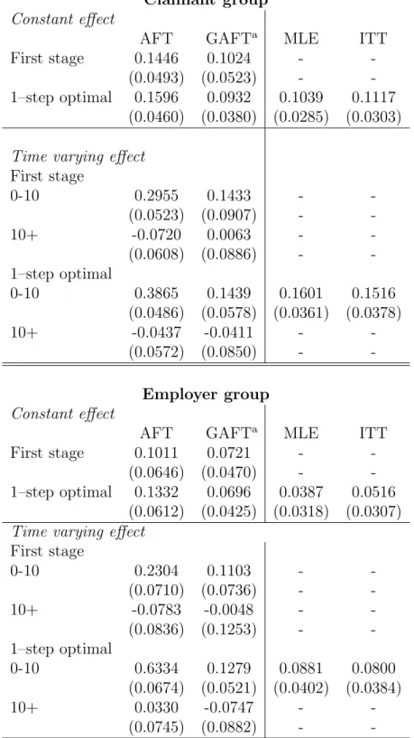
Table 2: Instrumental Variable Linear Rank estimates for the coefficient of the Bonus
Claimant group
Constant effect
AFT GAFTa MLE ITT
First stage 0.1446 0.1024 - -(0.0493) (0.0523) - -1–step optimal 0.1596 0.0932 0.1039 0.1117
(0.0460) (0.0380) (0.0285) (0.0303) Time varying effect
First stage 0-10 0.2955 0.1433 - -(0.0523) (0.0907) - -10+ -0.0720 0.0063 - -(0.0608) (0.0886) - -1–step optimal 0-10 0.3865 0.1439 0.1601 0.1516 (0.0486) (0.0578) (0.0361) (0.0378) 10+ -0.0437 -0.0411 - -(0.0572) (0.0850) - -Employer group Constant effect
AFT GAFTa MLE ITT
First stage 0.1011 0.0721 - -(0.0646) (0.0470) - -1–step optimal 0.1332 0.0696 0.0387 0.0516
(0.0612) (0.0425) (0.0318) (0.0307) Time varying effect
First stage 0-10 0.2304 0.1103 - -(0.0710) (0.0736) - -10+ -0.0783 -0.0048 - -(0.0836) (0.1253) - -1–step optimal 0-10 0.6334 0.1279 0.0881 0.0800 (0.0674) (0.0521) (0.0402) (0.0384) 10+ 0.0330 -0.0747 - -(0.0745) (0.0882) -
-aGAFT piecewise constant intervals: 0–2, 2–4, 4–6, 6–10, 10–25,
25→; Notes: Standard error in brackets.
The estimation results for the bonus effects are reported in Table 2. The results for the piecewise constant λ can be found in Table 3. A comparison of the results that AFT
overesti-Table 3: Estimated λ in GAFT model for the Bonus data Claimant
Constant Bonus effect Time varying Bonus effect interval first opt. first opt. 0–2 0.8098 0.7500 0.8625 0.9328 (0.4638) (0.2052) (0.5262) (0.2409) 2–4 0.3146 0.2348 0.3542 0.2309 (0.3691) (0.1462) (0.4048) (0.1799) 4–6 -0.0782 -0.0415 -0.0390 0.0318 (0.2646) (0.1220) (0.3015) (0.1552) 6–10 -0.2743 -0.1859 -0.2341 -0.2085 (0.2392) (0.1133) (0.2807) (0.1369) 10–25 -0.6868 -0.6655 -0.6077 -0.6345 (0.1626) (0.1006) (0.1758) (0.1261) Employer
Constant Bonus effect Time varying Bonus effect interval first opt. first opt. 0–2 0.7095 0.8929 0.7088 0.5647 (0.3063) (0.1450) (0.4375) (0.1716) 2–4 0.2540 0.4451 0.2542 0.1464 (0.2134) (0.0939) (0.3344) (0.1227) 4–6 -0.1217 -0.1178 -0.1195 0.0875 (0.2008) (0.0925) (0.2330) (0.1050) 6–10 -0.4552 -0.2707 -0.4526 -0.4098 (0.1516) (0.0751) (0.2255) (0.0975) 10–25 -0.7492 -0.6826 -0.7180 -0.6057 (0.0971) (0.0372) (0.1015) (0.0491)
mates the effect and that both ML and ITT estimators underestimate the effect of the employer bonus. The results clearly indicate that the bonuses only influence the chances to find a job in the first ten weeks. This is in line with the bonus eligibility period: those who find a job after that period would not get the bonus. The effect of the Claimant Bonus increases from about 10% higher probability to find a job at every unemployment duration to about 15% higher probability to find a job in the first ten weeks (and no effect thereafter). The bonus for the Em-ployer group raises the job finding probability with about 7% at every unemployment duration or with about 12% in the first ten weeks of unemployment. From Table 3 we can derive that the shape of the estimated λ’s indicate a U–shaped λ.
An indication that the AFT is not the right model is the difference between the first stage and one–step optimal estimators for the AFT model. For a correctly specified model both estimators are consistent and, therefore, do not differ much. In the GAFT model the first stage and one–step estimator are of the same magnitude. The estimated standard errors of the latter are, as expected, substantially lower in most situations.
In the GAFT (and AFT) model the treatment effect of the bonus is defined in terms of the change in the quantiles dtq(1)/dtq(0) , see (11). In an AFT model with a time-constant
treatment coefficient for the bonus the treatment effect is constant. In a GAFT model the λ
function influences the treatment effect. Using the distribution of U0, already calculated to
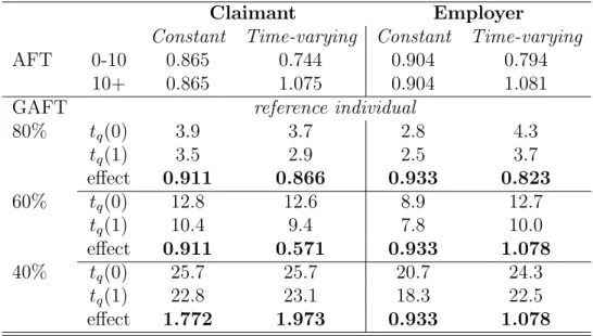
estimate the optimal IVLR and the variance-covariance matrix, we can derive the treatment effect of the bonus in the GAFT depending on the quantile of the distribution. In Table 4 we present the effect for the 80%, 60% and 40% survival, together with the AFT treatment effect (first stage). Figure 1 and Figure 2 depict the change over the survival quantile of the treatment effect of the bonus in the GAFT model.
Table 4: Effect of the Bonus on the length of unemployment duration
Claimant Employer
Constant Time-varying Constant Time-varying AFT 0-10 0.865 0.744 0.904 0.794
10+ 0.865 1.075 0.904 1.081 GAFT reference individual
80% tq(0) 3.9 3.7 2.8 4.3 tq(1) 3.5 2.9 2.5 3.7 effect 0.911 0.866 0.933 0.823 60% tq(0) 12.8 12.6 8.9 12.7 tq(1) 10.4 9.4 7.8 10.0 effect 0.911 0.571 0.933 1.078 40% tq(0) 25.7 25.7 20.7 24.3 tq(1) 22.8 23.1 18.3 22.5 effect 1.772 1.973 0.933 1.078
0 0.2 0.4 0.6 0.8 1 1.2 1.4 1.6 1.8 2 0.9 0.85 0.8 0.75 0.7 0.65 0.6 0.55 0.5 0.45 0.4 0.35 0.3 0.25 Survival quantile Claimant constant Employer constant
Figure 1: Treatment effect of Bonus on quantiles of unemployment duration, constant treatment coefficient 0 0.2 0.4 0.6 0.8 1 1.2 1.4 1.6 1.8 2 0.9 0.85 0.8 0.75 0.7 0.65 0.6 0.55 0.5 0.45 0.4 0.35 0.3 0.25 Survival quantile Claimant time-varying Employer time-varying
Figure 2: Treatment effect of Bonus on quantiles of unemployment duration, treatment coeffi-cient that changes after 10 weeks
Note that an effect smaller than one indicates that the bonus decreases the duration till re-employment and an effect bigger than one increases the duration. We see from the table (and more pronounced in Figure 1 ) that even for a time-constant γ the effect of the bonus on the unemployment duration in the GAFT changes with the duration. The huge spike in the effect at the survival quantile of 40% for the claimant group is because re–employment rate of unemployment durations exhibits a spike just before the time that unemployment benefits are exhausted at 25 weeks. For the individuals in the control group the 40% survival time is just before 26 weeks, while in the claimant bonus group it is at 23 weeks. Thus the control group individuals are in the re-employment spike while the claimant bonus group are not. The interval boundaries of the other intervals of λ also cause, although not as pronounced, spikes. These spikes are downward because the λ is jumping to a lower level at these boundaries. The spikes are also visible in the effect of a time-varying coefficient of the bonus, see Figure 2. Here, the change inγ at a duration of 10 weeks, after which the coefficient is negative, is reflected is a upward shift of the effect curve.
6
Conclusion
In this article we proposed and implemented an instrumental variable estimation procedure to estimate treatment effects for duration outcomes based on a Generalized Accelerated Failure Time (GAFT) model. The GAFT model is based on a transformation of the durations that encompasses both the Accelerated Failure Time (AFT) and the Mixed Proportional Hazards (MPH) model. The interpretation of the treatment effect in the GAFT model is in terms of shifting the quantiles of the distribution.
The proposed Instrumental Variable Linear Rank (IVLR) estimation procedure is based on the inverse of an extended rank-test. It exploits that for the population parameters any (weight)function of the instrument is independent of the distribution of the transformed dura-tions. It implies that the expected difference between the value of the weight function to the average of the weight functions for those individuals that are still under observation on the transformed duration scale is zero. The estimation procedure is related to the Rank Preserving Structural Failure Time Model estimator of Robins and Tsiatis (1991). The main difference with the RPSFT-model is that it assumes an AFT model while the IVLR allows for the more general GAFT-model, that includes duration dependence. The procedure is also related to the 2 stage Linear Rank (2SLR) estimation procedure of Bijwaard and Ridder (2005). The 2SLR
assumes an MPH model and is a 2-steps procedure, while the IVLR is a one-step procedure. The IVLR is based on a vector of mean restrictions and, therefore, it is related to the well-known GMM estimation procedure. Similar to the GMM estimation choosing the right weight functions can improve the efficiency. However, again similar to the GMM, these optimal weight functions are not directly observable. Fortunately, an adaptive (or even 2 step) procedure can provide the efficient IVLR. We show that a counting process framework simplifies the derivation and interpretation of the IVLR. The counting process framework also enables us to derive the large sample properties of the IVLR.
The empirical application shows that the ML and ITT estimates give downward biased treatment effects if the there is selective treatment choice. We also find that incorrectly assuming an AFT model can give misleading conclusions about the treatment effects of a bonus on the unemployment duration. In the Illinois bonus re-employment experiment many unemployed found a job just before their UI-benefits expires. This induces a spike in the re-employment hazard. In the GAFT model, even with a constant treatment coefficient, such a spike leads to an effect that changes over the quantiles. This has important implications for the evaluation of the treatment effect.
There are several issues that need further research. First, the current approach to adjust for endogenous censoring implies loss of information and depends on the (unknown) parameters of the model. An important improvement would be to find a method to adjust for endogenous censoring that is parameter independent and minimizes the loss of information. Further research on more general censoring patterns also deserve attention. A second issue for further research is the extension of the IVLR to recurrent duration data, like repeated unemployment spells.
References
Abbring, J. H. and G. J. van den Berg (2003). The non–parametric identification of treatment effects in duration models. Econometrica 71, 1491–1517.
Abbring, J. H. and G. J. van den Berg (2005). Social experiments and instrumental variables with duration outcomes. Tinbergen Institute, discussion paper, TI 2005–47.
Andersen, P. K., O. Borgan, R. D. Gill, and N. Keiding (1993).Statistical Models Based on Counting Processes. New York: Springer–Verlag.
Ashen-felter and D. Card (Eds.), Handbook of Labor Economics, Volume 3A, Chapter 23, pp. 1277–1366. Amsterdam: North–Holland.
Ashenfelter, O., D. Ashmore, and O. Deschˆene (2005). Do unemployment insurance recipi-ents actively seek work? Evidence from randomized trials in four U.S. states. Journal of Econometrics 125, 53–75.
Bijwaard, G. E. and G. Ridder (2005). Correcting for selective compliance in a re–employment bonus experiment. Journal of Econometrics 125, 77–111.
Br¨ann¨as, K. (1992).Econometrics of the Accelerated Duration Model. Ume˚a: Solfj¨adern Offset AB.
Chesher, A. (2002). Semi–parametric identification in duration models. CeMMAP, working paper, CWP20/02.
Cox, D. R. and D. Oakes (1984).Analysis of Survival Data. London: Chapman and Hall.
Ham, J. C. and R. J. LaLonde (1996). The effect of sample selection and initial conditions in duration models: Evidence from experimental data on training. Econometrica 64, 175– 205.
Han, A. K. (1987). Non–parametric analysis of a generalized regression model: The maximum rank correlation estimator. Journal of Econometrics 35, 303–316.
Hausman, J. A. and T. M. Woutersen (2005). Estimating a semi–parametric duration model without specifying heterogeneity. CeMMAP, working paper, CWP11/05.
Heckman, J. J., R. J. LaLonde, and J. A. Smith (1999). The economics and econometrics of active labor market programs. In O. Ashenfelter and D. Card (Eds.),Handbook of Labor Economics, Volume 3A, Chapter 31, pp. 1866–2097. Amsterdam: North–Holland.
Holland, P. W. (1986). Statistics and causal inference (with discussion).Journal of the Amer-ican Statistical Association 81, 945–970.
Kalbfleisch, J. D. and R. L. Prentice (2002). The Statistical Analysis of Failure Time Data (second edition). John Wiley and Sons.
Klein, J. P. and M. L. Moeschberger (1997).Survival Analysis: Techniques for Censored and Truncated Data. New York: Springer–Verlag.
Koenker, R. and Y. Bilias (2001). Quantile regression for duration data: A reappraisal of the Pennsylvania reemployment bonus experiments. Empirical Economics 26, 199–220.