Johns Hopkins University, Dept. of Biostatistics Working Papers
11-1-2004
Spatially Adaptive Bayesian P-Splines with
Heteroscedastic Errors
Ciprian M. Crainiceanu
Johns Hokins Bloomberg School of Public Health, Department of Biostatistics, [email protected]
David Ruppert
School of Operational Research & Industrial Engineering, Cornell University, [email protected]
Raymond J. Carroll
Department of Statistics, Texas A&M University, [email protected]
This working paper is hosted by The Berkeley Electronic Press (bepress) and may not be commercially reproduced without the permission of the copyright holder.
Copyright © 2011 by the authors Suggested Citation
Crainiceanu, Ciprian M.; Ruppert, David; and Carroll, Raymond J., "Spatially Adaptive Bayesian P-Splines with Heteroscedastic Errors" (November 2004).Johns Hopkins University, Dept. of Biostatistics Working Papers.Working Paper 61.
Spatially Adaptive Bayesian P-Splines With
Heteroscedastic Errors
Ciprian M. Crainiceanu
∗David Ruppert
†Raymond J. Carroll
‡November 9, 2004
Abstract
An increasingly popular tool for nonparametric smoothing are penalized splines (P-splines) which use low-rank spline bases to make computations tractable while main-taining accuracy as good as smoothing splines. This paper extends penalized spline methodology by both modeling the variance function nonparametrically and using a spatially adaptive smoothing parameter. These extensions have been studied before, but never together and never in the multivariate case. This combination is needed for satisfactory inference and can be implemented effectively by Bayesian MCMC. The variance process controlling the spatially-adaptive shrinkage of the mean and the vari-ance of the heteroscedastic error process are modeled as log-penalized splines. We discuss the choice of priors and extensions of the methodology, in particular, to multi-variate smoothing using low-rank thin plate splines. A fully Bayesian approach provides the joint posterior distribution of all parameters, in particular, of the error standard deviation and penalty functions. In the multivariate case we produce maps of the stan-dard deviation and penalty functions. Our methodology can be implemented using the Bayesian software WinBUGS.
Keywords: Knot selection; MCMC; Mixed models; Multivariate smoothing; Spatially adap-tive penalty; Thin-plate splines.
∗Assistant Professor, Department of Biostatistics, Johns Hopkins University, 615 N. Wolfe St. E3037
Baltimore, MD 21205 USA. E-mail: [email protected]
†Andrew Schultz Jr. Professor of Engineering and Professor of Statistical Science, School of
Opera-tional Research and Industrial Engineering, Cornell University, Rhodes Hall, NY 14853, USA. E-mail: [email protected]
‡Distinguished Professor of Statistics and Professor of Nutrition and Toxicology, Department of
car-1
Introduction
P-splines (Eilers and Marx, 1996; Ruppert, Wand, and Carroll, 2003) have become a popular nonparametric tool. Their success is due mainly to the use of low rank bases, which makes computations tractable. Also P-splines can be viewed as mixed models and fit with widely available statistical software (Ngo and Wand, 2003; Crainiceanu, Ruppert and Wand 2004). Bayesian penalized splines (Ruppert, Wand, and Carroll, 2003; Lang and Brezger, 2004) use a stochastic process model as a prior for the regression function. The usual Bayesian assumes that both this processes and the errors are homoscedastic.
The P-spline methodology has been extended to heteroscedastic errors (Ruppert, Wand, and Carroll, 2004) and also to spatially adaptive penalty parameters (Ruppert and Carroll, 2000; Baladandayuthapani, Mallick, and Carroll, 2004; Lang and Brezger, 2004). However, this is the first paper to combine these features. We show that this combination is important. Since the penalty parameter is the ratio of the error variance to the prior variance on the mean function, it is true that spatially varying penalties can adapt to both spatial heterogeneity of both the mean function and the error variance, at least for the purpose of estimation. However, for correct inference it is necessary to separate the spatial heterogeneity of the mean and of the error variance, and the innovation of this paper is to do that. Implementation of this extension was not straightforward because of technical problems such as slow MCMC mixing and sensitivity to the choice of prior, but we were able develop an algorithm that works satisfactorily in practice.
Our methodology can be extended to almost any of the P-spline model, for example, those in Ruppert, Wand, and Carroll (2003) such as additive models, varying coefficient models, interaction models, and multivariate smoothing. As an illustration, we also study low rank thin plate (multivariate) splines. As in the univariate case we model the mean, the variance and the smoothing functions nonparametrically and estimate them from the data using a fully Bayesian approach. The computational advantage of low rank over full rank smoothers becomes even greater in more than one dimension.
Section 2 provides a quick introduction to P-splines and their connections with mixed models. Section 3 discusses the choice of priors for P-spline regression. Section 4 pro-vides simultaneous credible bounds for mean and variance functions and their derivatives. Sections 5 provides an example and comparisons with simpler techniques and in Section 9 we compare our proposed methodology to the one proposed by Baladandayuthapani et al. (2004) for adaptive univariate P–spline regression. Section 7 describes the extension to multivariate smoothing and in Section 8 we present an example of bivariate smoothing with heteroscedastic errors and spatially adaptive smoothing. Section 9 compares our mul-tivariate methodology with other adaptive surface fitting methods. Section 10 presents the full conditional distributions and discusses our implementation of models in WinBUGS and
MATLAB.
2
P-Splines regression and mixed models
Consider the regression equation yi =m(xi) +²i, i= 1, . . . , n,where the²i are independent N(0, σ2
²,i) and the mean is modeled as
m(x) =m(x,θX) = β0 +β1x+· · ·+βpxp + Km X k=1 bk(x−κmk) p + , where β = (β0, . . . , βp)T, b = (b1, . . . , bKm)T, θX = (β T,bT)T, κm 1 < κm2 < . . . < κmKm are
fixed knots, and ap+ denotes {max(a,0)}p. Following Gray (1994) and Ruppert (2002), we take Km large enough (e.g., 20) to ensure the desired flexibility.
To avoid overfitting the bk ∼ N{0, σ2b(κmk)} and ²i ∼ N{0, σ²2(xi)} are shrunk towards zero by an amount controlled byσ2
b(·) andσ2²(·), which vary across the range ofx. In Sections 2.1 and 2.2 σ2
²(xi) and σ2b(κmk) are modeled using log-spline models. The P-spline model can be written in linear mixed model form as
yi = β0+β1xi+. . .+βpxpi + PKm k=1bk(xi−κmk)p++²i ; bk ∼ N{0, σb2(κmk)}, k = 1, . . . , Km ; ²i ∼ N{0, σ²2(xi)}, i= 1, . . . , n , (1) wherebkand²i are mutually independent given (σ²2, σb2), andσ²2 andσ2b are smooth functions
that will be modeled as logsplines. Denote by X the n × (p+ 1) matrix with the ith
row equal to Xi = (1, xi, . . . , xpi) and by Z the n × Km matrix with ith row equal to Zi ={(xi−κm1 )p+, . . . ,(xi−κmKm)
p
+},Y = (y1, . . . , yn)T and²= (²1, . . . , ²n)T. Model (1) can be rewritten in matrix form as
Y =Xβ+Zb+², E µ b ² ¶ = µ 0 0 ¶ , Cov µ b ² ¶ = µ Σb 0 0 Σ² ¶ , (2)
where the joint conditional distribution ofband²givenΣb andΣ²is assumed normal. Theβ parameters are treated as fixed effects. The covariance matricesΣb andΣ² are diagonal with the vectors {σ2
b(κm1 ), . . . , σb2(κmKm)} and {σ
2
²(x1), . . . , σ2²(xn)} as main diagonals respectively. For this model E(Y) =Xβ and cov(Y) = Σ²+ZΣbZT.
2.1
Error variance function estimation
Ignoring heteroscedasticity may lead to incorrect inferences and inefficient estimation, espe-cially when the response standard deviation varies over several orders of magnitude. More-over, understanding how variability changes with the predictor may be of intrinsic interest (Carroll, 2003).
Transformation can stabilize the response variance when the conditional response variance is a function of the conditional expectation (Carroll and Ruppert, 1988), but in other cases one needs to estimate it by modeling the variance as a function of the predictors.
We model the variance function as a loglinear mixed model ½ log{σ2 ²(xi)} = γ0 +. . .+γpxpi + PK² s=1cs(xi−κ²s)p+ cs ∼ N(0, σ2c), s= 1, . . . , K² , (3) where the γ are fixed effects and κ²
1 <· · ·< κ²K² are knots. The normal distribution of the
cs parameters shrinks them towards 0 and ensures stable estimation.
2.2
Smoothly varying local penalties
Following Baladandayuthapani et al. (2004), we model σ2 b(·) as ½ log{σ2 b(x)} = δ0+. . .+δqxq+ PKb s=1ds(x−κbs)q+ ds ∼ N(0, σ2d), s= 1, . . . , Kb , (4)
where the δ’s are fixed effects, the ds’s are mutually independent, and {κbs}Ks=1b are knots. The particular case of a global smoothing parameter corresponds to the case when the spline function is a constant, that is log{σ2
b(κms )}=δ0.
Ruppert and Carroll (2000) proposed a “local penalty” model similar to (4). Baladan-dayuthapani, Mallick and Carroll (2003) developed a Bayesian version of Ruppert and Car-roll’s (2000) estimator and showed that their estimator is similar to Ruppert and CarCar-roll’s in terms of mean square error and outperforms other Bayesian methods. Lang, Fronk and Fahrmeir (2004) consider locally adaptive dynamic models and find that their method is roughly comparable to the method of Ruppert and Carroll (2000) in terms of MSE and coverage probability.
In Lang and Brezger’s (2004) prior for the bk, the nonconstant variance is independent from knot to knot, since the variances of the bk are assumed to be independent inverse-gammas. In contrast, with our model there is dependence so that if the variance is high at one knot then it is high at neighboring knots. Stated differently, the Lang and Brezger model is one of random heteroscedasticity and ours of systematic heteroscedasticity. Both types of priors are sensible and will have applications, but in any specific application it is likely that one of the two will be better. For example, Lang and Brezger find that for “doppler type” functions, e.g., the severe spatial heterogeneity function in Ruppert and Carroll (2001), their estimator is not quite as good as Ruppert and Carroll’s and that the coverage of their credible intervals are not so accurate either. It is not hard to understand why. Doppler type functions that oscillate more slowly going from left to right are consistent with a prior variance for the bk that is monotonically decreasing, exactly the type of prior included in our model but not Lang and Brezger’s.
2.3
Choice of spline basis, number and spacing of knots, and
penalties
For concreteness, we have made some specific choices about the spline basis, number and knot spacings, and form of the penalty. In terms of model formulation, the choice of spline basis in the model is not important since an equivalent basis gives the same model and the basis used in computations need not be the same as the one used to express the model. However, spline basis are very different in terms of computational stability. For example, cubic thin plate spline (Ruppert, Wand and Carroll 2003, pp. 72–74) provide much better MCMC convergence and mixing properties than the truncated polynomial basis. When one uses good starting points for the MCMC simulation the truncated polynomial and the cubic thin plate spline bases produced very similar results. In more than one dimension, the tensor product of truncated polynomials proved even more unstable and we preferred using low rank radial smoothers (see Section 7).
The penalty we use is somewhat different than that of Eilers and Marx (1996) and also somewhat different from the penalties used by smoothing splines. We believe that the penalty parameter, not the form of the penalty, is the crucial choice, so we have concentrated on the former, in particular on spatially-adaptive modeling of the penalty parameter.
In this paper we use knots to model the mean, variance and spatially adaptive smoothing parameter. The methodology described here does not depend on the number of knots. For example one could use a knot at each observation for each of the three functions.
Although we use quantile knot spacings, the best type of knot spacings is controversial. Eilers and Marx (1996) state that “Equally-spaced knots are always to be preferred.” In contrast, Ruppert, Wand, and Carroll (2003) used quantile-spacing in all of their examples, though they did not make any categorical statement that quantile–spacing is always to be preferred. Although the main focus of this paper is not the choice of knot-spacings, we felt it was necessary to discuss this issue here.
When σ2
b(x) is a constant, then the knot spacings determine the form of the prior on m. To appreciate this, note that the prior for m has a simple form: m(p) is a random walk taking jumps at the knots. The jumps are independent N(0, σ2
b). If the knots are equally spaced, then the prior makes m(p) spatially homogeneous in that the variance of the sum of its jumps in an interval is nearly proportional to the length of the interval. The prior can be viewed as a discrete approximation to the model
dm(p)(x) =σdW(x), (5)
whereW is a standard Wiener process. Model (5) is the prior for smoothing splines (Wahba, 1990). If the knots are not equally spaced, then m(p) changes more rapidly in regions where the xi (and therefore the knots) are relatively dense so our prior is a discrete approximation
to the model
dm(p)(x) = σ
bf(x)dW(x) (6) where f(x) is some measure of the density of {x1, . . . , xn}, e.g., is the probability density function of the xi if they are random and iid. For non-random xi, f(x) might be a kernel density estimator computed from the xi. There is no compelling reason to assume spatial homogeneity, that is, model (5), especially since it is not invariant to nonlinear transforma-tions of the xi. However, there is also no compelling reason to assume that m(p) changes most rapidly where the data are most dense, that is, that (6) holds.
Fortunately, whenσ2
b is not constant, the knot spacings do not determine the form of the prior because the effect of spacing on the prior can be subsumed into the form of σ2
b. Stately differently, if σ2
b depends on x, then (5) and (6) can both hold but with different σb(x). Our conclusion is that quantile knot spacing works well and can be recommended in practice.
2.3.1 A Monte Carlo study of knot spacing
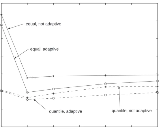
The motivation behind quantile knot spacing is to use more densely spaced knots where there is more information (more data). Suppose that the regression function is spatially het-erogenous and, in fact, has more “features” in regions where the data are dense. This is not an unreasonable assumption, especially when the xi are chosen by design and there is some prior knowledge of where m will have the most “features.” In such cases, quantile-spacing allows the penalized spline to fit fine detail where the features occur without undersmooth-ing elsewhere. The followundersmooth-ing simulation example illustrates this behavior. The purpose of the example is not to argue that quantile spacing is always to be preferred. We doubt that any type of spacing is always best, and Eilers and Marx (2004) provide an interesting ex-ample where equally-spaced knots seem superior to quantile spacing; see their Figure 13. The purpose of the example is, rather, to show that quantile spacing can work better than equal-spacing knots in some problems. In this example, we used non-Bayesian estimators since they are much faster to compute and the relative performance was not expected to depend on whether the estimator was Bayesian or not.
In this example, there aren = 100 observations with covariate valuesxi = (i−1/99)4, i= 1, . . . ,100 and response yi = 10 sin{60xi/(1 + 3xi)}+²i with ²i ∼N(0,9). Thexi are much more dense near 0 than near 1 and the regression function oscillates faster in this region. There were 1000 simulated data sets. For each estimator, the regression function was es-timated on a 1000–point grid. The squared error was averaged over this grid and then averaged over the 1000 data sets to produce a MASE (mean average squared error). We used quadratic splines and the number of knots was varied as 10, 15, 20, 30, and 40. There were four estimators. “Equal, not adaptive” is the Eilers and Marx estimator computed using the MATLAB program in Eilers and Marx (1996) with the order of the penalty equal
to 2. This estimator uses B-splines and equally spaced knots. The second estimator, called “Quantile, not adaptive,” used quantile spacing of the knots and a penalty of the sum of the squared jumps in the second derivative of the spline; this is equivalent to penalizing the sum of the squared coefficients of the truncated power functions. “Quantile, adaptive” and “Equal, adaptive” are the Ruppert and Carroll (2000) estimators with quantile and equal knot spacings, respectively. In all cases the penalty parameter was selected by gener-alized cross validation. In this example, quantile spacings outperformed equal knot spacings noticeably, especially for non-adaptive penalties; see Figure 1.
This example is an extreme case, as is the example of Eilers and Marx (2004) mentioned previously. We find in the majority of examples that both equal and quantile spacings work perfectly well. There is a long history of success with the quantile spacings, since smoothing splines are a special case of quantile spacing with a knot at each data point.
All univariate examples in this paper will use quantile knot spacing.
3
Prior Specification
Any smoother depends heavily on the choice of smoothing parameter, and for P-splines in a mixed model framework, the smoothing parameter is the ratio of the error variance to the prior variance on the mean (Ruppert, Wand and Carroll, 2003). The smoothness of the fit depends on how these variances are estimated. For example, Crainiceanu and Ruppert (2004) showed that, in finite samples, the (RE)ML estimator of the smoothing parameter is biased towards oversmoothing and Kauermann (2002) obtained corresponding asymptotic results for smoothing splines.
In Bayesian mixed models, the estimates of the variance components are known to be sensitivity to the prior specification, e.g., see Gelman (2004). To study the effect of this sensitivity upon Bayesian P-splines, consider model (1) with one smoothing parameter and homoscedastic errors so that σ2
b and σ2² are constant. In terms of the precision parameters τb = 1/σb2 and τ² = 1/σ2², the smoothing parameter isλ =τ²/τb =σb2/σ2² and a small (large)
λ corresponds to oversmoothing (undersmoothing).
3.1
Priors on the fixed effects parameters
It is standard to assume that the fixed effects parameters, βi, are apriori independent, with prior distributions either [βi]∝1 orβi ∝N(0, σβ2), whereσβ2 is very large. In our applications we used σ2
β = 106, which we recommend if x and y have been standardized or at least have standard deviations with order of magnitude one.
For the fixed effects γ and δ used in the log-spline models (3) and (4) we also used independent N(0,106) priors. When this prior is not consistent with the true value of the parameter, a possible strategy is to fit the model using a given set of priors and obtain
the estimators bγ, bσbγ, bδ and bσbδ. We could then use independent priors N(bγ,106σbbγ2) and N(bδ,106σb2
b
δ) forγ and δ respectively.
3.2
Priors on the precision parameters
As just mentioned, the priors for the precisions τb and τ² are crucial. We now show how critically the choice of τb may depend upon the scaling of the variables. The gamma family of priors for the precisions is conjugate. If [τb] ∼Gamma(Ab, Bb) and, independently of τb, [τ²]∼Gamma(A², B²) where Gamma(A, B) has mean A/B and variance A/B2, then
[τb|Y,β,b, τ²]∼Gamma µ Ab+ Km 2 , Bb+ ||b||2 2 ¶ (7) and [τ²|Y,β,b, τ²]∝Gamma µ A²+ n 2, B²+ ||Y −Xβ−Zb||2 2 ¶ . Also, E(τb|Y,β,b, τ²) = Ab+Km/2 Bb+||b||2/2 , Var(τb|Y,β,b, τ²) = Ab+Km/2 (Bb+||b||2/2)2 , and similarly for τ|².
The prior does not influence the posterior distribution of τ² when both Ab and Bb are small compared to Km/2 and ||b||2/2 respectively. Since the number of knots is Km ≥ 1 and in most problems considered Km ≥ 5, it is safe to choose Ab ≤ 0.01. When Bb << ||b||2/2 the posterior distribution is practically unaffected by the prior assumptions. When Bb increases compared to ||b||2/2, the conditional distribution is increasingly affected by the prior assumptions. E(τb|Y,β,b, τ²) is decreasing in Bb so large Bb compared to ||b||2/2 correspond to undersmoothing. Since the posterior variance of τb is also decreasing in Bb a poor choice of Bb will likely result in underestimating the variability of the smoothing parameter λ = τ²/τb causing too narrow confidence intervals for m. The condition Bb << ||b||2/2 shows that the “noninformativeness” of the gamma prior depends essentially on the scale of the problem.
To show the possible severity of these effects consider the LIDAR example in Section 5. We consider model (1) with a global smoothing parameter and homoscedastic error. We used quadratic splines with 30 knots. Figure 2 shows the effect of four mean-one Gamma priors for the precision of the truncated polynomial parameters. The variances of these priors are 10, 103, 106, and 1010 respectively. Obviously, the first two inferences provide severely under smoothed, almost indistinguishable, posterior means. The third graph is much smoother but still exhibits roughness especially in the right hand side of the plot, while the fourth graph displays a pleasing smooth pattern, consistent with our frequentist inference. Using either prior distribution one obtains that the posterior mean of ||b||2/2 is of order 10−6 to 10−5. This explains why values of Bb larger than 10−6 proved inappropriate for this problem.
The size of ||b||2/2 depends upon the scaling of the x and y variables and in the case of the LIDAR data ||b||2/2 is small because the standard deviation of x is much larger than the standard deviation of y. If y is rescaled to ayy and x to axx, then the regression function becomesaym(axx) whosep-th derivative isayapxm(p)(axx) so that ||b||2/2 is rescaled by the factor a2
ya2px . Thus, ||b||2/2 is particularly sensitive to the scaling of x. The size of ||b||2/2 also depends onK
m. The integral of m(p) over the range of x will be approximately PKm
k=1bk≈ √
Kmσb, we can expect thatσ2b ∝(Km)−1and the smoothing parameter should be
proportional to Km. For the LIDAR data, the GCV chosen smoothing parameter is 0.0095,
0.0205, 0.0440, and 0.0831 forKm equal to 15, 30, 60, and 120, respectively, so as expected
the smoothing parameter approximately doubles as Km doubles.
Practical experience with LMMs for longitudinal or clustered data should be applied with caution to P-splines. In a mixed effects model ||b||2 is an estimator of K
mσ2b. For longitudinal data Kmσb2 would generally be large becauseKm is the number of subjects with constant subject effect variance σ2
b. As just discussed, for a P-spline Kmσb2 should be nearly independent of Km and could be quite small.
Figure 3 presents the same type of results as Figure 2 for Gamma priors for the precision parameter τb with the mean held fixed at 10−6 and variances equal to 10, 103, 106, and 1010 respectively. These prior distributions have a much smaller effect on the posterior mean of the regression function. The fit seems to be undersmooth when the variance is 10. Clearly, when the variance increases the fit becomes smooth indicating that a value of the variance larger than 103 will produce a reasonable fit.
It is sometimes believed that a Gamma(A, B) prior is non-informative if both A and B are sufficiently small. However, such non-informative priors are not flat. To illustrate this, consider a small right neighborhood of zero I0 = (0,10−6] and denote byPA the prob-ability distribution of a Gamma(1/A,1/A) distribution. Then P10(I0) = 0.21, P103(I0) = 0.98, P106(I0) = 0.99997, P1010(I0) ≈ 1. For this type of distributions the large variance is not due to the “flatness” of the prior but to the extremely rare very large values.
A similar discussion holds true forτ² but now largeB² corresponds to oversmoothing and τ² does not depend on the scaling ofx. In applications it is less likely that B² is comparable in size to ||Y −Xβ−Zb||2, because the latter is an estimator ofnσ2
². If ˆσ²2 is an estimator of σ2
² a good rule of thumb is to use values of B² smaller than nσˆ2²/100. This rule should work well when ˆσ2
² does not have an extremely large variance.
Alternative to gamma priors are discussed by, for example, Natarajan and Kass (2000) and Gelman (2004). These have the advantage of requiring less care in the choice of the hyperparameters. However, we find that with reasonable care, the conjugate gamma priors can be used in practice. Nonetheless, exploration of other prior families for P-splines would be well worthwhile, though beyond the scope of this paper.
4
Simultaneous Credible Bounds
Let f(·) be either m(·), log{σ2²(·)}, log{σb2(·)}, or a derivative of order q, 1≤ q ≤ p, of one of these functions. It is straightforward to use MCMC output to construct simultaneous credible bounds on f over an arbitrary finite interval [x1, xN]. Typically, x1 and xN would be the smallest and largest observed values of x.
Let x1 < x2 < · · · < xN be a fine grid of points on this interval. Let E{f(xi)} and SD{f(xi)}be the posterior mean and standard deviation off(xi) estimated from a MCMC sample. LetMα be the (1−α) sample quantile of max1≤i≤N
¯
¯[f(xi)−E{f(xi)}]/SD{f(xi)}¯¯ computed from the realizations of f in the MCMC sample. Then I(xi) = E{f(xi)} ± MαSD{f(xi)}, i = 1, . . . , N, are simultaneous credible intervals. For N large, the upper and lower limits of these intervals can be connected to form simultaneous credible bands. In the remainder of this paper we only report simultaneous credible bounds for the functions and their derivatives. In the examples considered in the following these bounds tend to be roughly 30–50% wider than pointwise credible bounds.
5
The LIDAR example
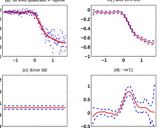
The data displayed in Figure 6-(a) are taken from Holst et al. (1996), who estimated the concentration of atmospheric mercury measured with LIDAR (Sigrist, 1994). The concen-tration is proportional to the derivative of the mean (with a negative and known constant of proportionality). Because of sizeable heteroscedasticity, the variance function must be estimated to obtain satisfactory credible intervals for the function and its derivative.
Three increasingly complex models were fit to the data. Model I uses a 30-knot quadratic P-spline for m and assumes that σ2
b and σ²2 are constant. Model II has the same structure for m and σ2
² as Model I but uses a linear log-P-spline with Kb = 4 knots to model log{σb2}. Model III differs from Model II in using a 30-knot quadratic P-spline for log{σ2
²(x)}.
To minimize the scale problems discussed in Section 3 we centered and standardized the covariate. The response was not standardized because its range is between −1 and 0, but in general we recommend standardizing the response. For simplicity we describe only the priors used for Model III. We assumed independent normal priors for the coefficients of the monomials βi ∼ N(0,106), γi ∼ N(0,106), i = 0, . . . , p, δi ∼ N(0,106), i = 0, . . . , q, and
independent inverse Gamma priors for the variance components σ2
c ∼ IGamma(10−3,10−3) and σ2
d ∼ IGamma(10−3,10−3). The full conditional distributions are in Section 10. Given our discussion in Section 3 we investigated whether this choice is non-informative enough
and found that much smaller values of a and b did not affect inference, probably due to
standardization of x.
standard deviation function is a constant and the credible intervals do not change from left to right. However, this assumption is contradicted by the data. Because m0(x,θ) = β
1 + 2β2x+ 2
PK
k=1bk(x−κk)+ is an explicit function of the parameters, its posterior distribution for each x can be easily estimated from the simulations.
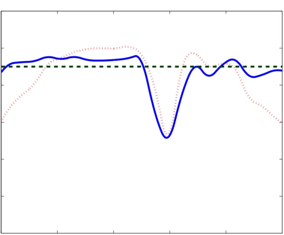
Figure 7 presents the results for model II. While the posterior means E(m|Y) from Models I and II are visually indistinguishable, E(m0|Y) has a sharper peak and wider 95%
credible intervals in Model II which has spatial adaptivity. An obvious question is whether differences are real. A rigorous test exceeds the scope of this paper, but we address a simpler related problem at the end of this section.
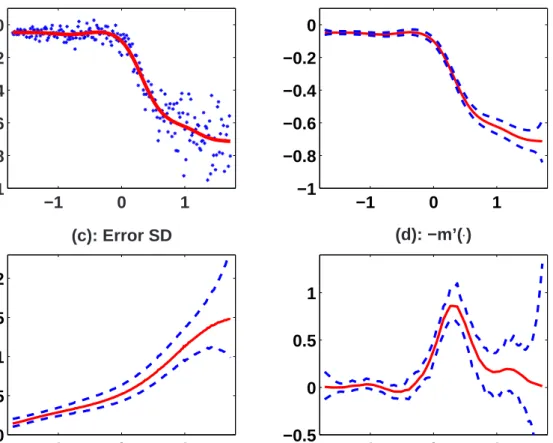
Figure 8 displays the same type of results for Model III. Figure 8-(b) shows that the simultaneous credible intervals for m are much narrower for small values ofx than for large x, in accordance with the non-constant variance seen in the data. This pattern is not present in Figures 6-(d) and 7-(d). Similar differences were reported by Ruppert, Wand and Carroll (2003) (see Section 14.3) who used a frequentist approach to estimate the error variance, but ignored the possible spatial variability of the smoothing parameter.
Figure 8-(c) shows that the standard deviation of the error process increases nonlinearly with the covariate and the variability around the standard deviation increases as well. As we mentioned, the object of inference is m0(·). Comparing the posterior mean of m(·) for
models I–III, one see little difference. However, there are noticable differences in the posterior means of −m0(·). For the local-penalty, Figures 7-(d) and 8-(d), have sharper peaks, which
suggests that the global penalty model corresponds to oversmoothing m0(·) in the middle
of the covariate range and undersmoothing m0(·) in the lower range. Second, when one
accounts for heteroscedasticity, Figure 8-(d), the function −m0(·) is smoother and the 95%
credible intervals are much narrower in the lower range of the covariate. This is probably due to the lower variability of the data in that region. Third, the credible intervals in the upper range of the covariate are slightly wider in 8-(d) compared to Figure 7-(d) and much wider compared to Figure 6-(d). These results are different from the results of Ruppert and Carroll, 2000, who did not account for the effect of heteroscedastic errors.
Figure 9 displays for model I with heteroscedastic errors and spatially adaptive smoothing parameter, the posterior mean and credible intervals for the logarithm of the shrinkage parameters, log(σ2
b). The shape of the posterior mean of log(σb2) suggests that a simpler linear trend may be suitable.
We fit a simplified model where the mean and log-variance of the errors are modeled as quadratic splines with Km = K² = 30 knots and log{σb2(κkb)} = δ0 +δ1κbk . Inference for this model produced plots very similar Figure 8 and are not reported here. To test whether δ1 >0 we used 500,000 simulations to obtainP(δ1 <0) = 0.04, indicating that the differences between the posterior means of −m0(·) using a global and a spatially adaptive
by the data.
6
Comparison with other univariate smoothers
Baladandayuthapani et al. (2004) present a comprehensive simulation study of their Bayesian spatially adaptive P–spline model, which is obtained as a particular case of our full model with constant error variance. The results of this study indicate that the method is comparable to or better than several other spatially adaptive Bayesian methods on a variety of data sets. Since we are unaware of any other estimation methodology that estimates jointly the nonparametric adaptive model for the mean and the nonparametric model for the error process, we will compare our methodology with that of Baladandayuthapani et al. (2004).
Consider the regression model
yi =m(xi) +²i
where ²i are independent mean zero normal errors and m(·) is the spatially heterogeneous regression function
m(x) = exp©−400(x−0.6)2ª+ 5
3exp{−500(x−0.75)
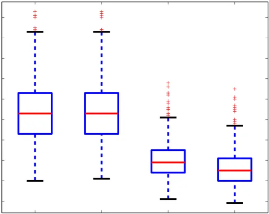
2}+ 2 exp{−500(x−0.9)2}. This function was also considered by Ruppert and Carroll (2000) and Baladandayuthapani et al. (2004) and it is roughly constant between [0,0.5] and has three sharp peaks at 0.6, 0.75 and 0.9. We consider n = 1,000 equally spaced xs on [0,1] and two different scenarios for the standard error of the error process: (a) σ²(x) = 0.5 for homoscedastic errors and (b) σ²(xi) = 0.5−0.8x+ 1.6(x−0.5)+. We used 500 simulations from these models and fit two spatially adaptive models: one that uses a constant variance and one that uses a log–P– spline model for the variance. For the mean and log–variance functions we used quadratic P-splines with Km = K² = 40 knots. For the log-variance corresponding to the shrinkage process we used Kb = 4 knots. We calculated the mean square error for each simulated data set as MSE =Pni=1{mb(xi)−m(xi)}2/n, where mb(x) is the posterior mean ofm(x) using a given model.
For case (a), σ²(x) = 0.5, the two models produced practically indistinguishable MSEs. The first boxplot (“ho-ho”) in Figure 4 corresponds to MSEs for the model using homoscedas-tic errors, while the second boxplot (“ho–he”) corresponds to heteroscedashomoscedas-tic errors. The average MSE over all x’s was AMSE = 0.0054, which is smaller than 0.0061 reported by Baladandayuthapani et al. (2004). The coverage probabilities of the 95% credible intervals were very similar for the two models for each value of the covariate, with a slight advantage in favor of the model using homoscedastic errors. The average coverage probability was 94.7% for the model with homoscedastic error and 93.5% for the model with heteroscedastic errors. These coverage probabilities are very similar to the ones reported by Baladandayuthapani et al. (2004) in their Figure 3.
For case (b), σ²(xi) = 0.5−0.8x+ 1.6(x−0.5)+, the heteroscedastic model substantially outperformed the homoscedastic model both in terms of MSE and coverage probabilities. The third boxplot (“he-ho”) in Figure 4 corresponds to MSEs for the model using homoscedastic
errors with AMSE= 0.003. The fourth boxplot (“he–he”) corresponds to heteroscedastic
errors with AMSE= 0.0026. In this situation it would be misleading to compare only the average coverage probability for the 95% credible intervals. Indeed, these averages are very close, 94.1% for the heteroscedastic and 93.0% for the homoscedastic method, but they are obtained from very different sets of pointwise coverage probabilities. Figure 5 displays the coverage probabilities for these two methods. Note that for the heteroscedastic method the coverage probability in the [0,0.5] interval is close to 95%. In the same interval the coverage probability for the homoscedastic method starts from around 0.8 and increases until it crosses the 95% target around 0.2. Moreover, in the interval [0.3,0.5] this coverage probability is estimated to be 1. This is due to the fact that on this interval σ²(x) decreases linearly from 0.5 to 0.1. Since the homoscedastic method assumes a constant variance, the credible intervals will tend to be shorter than nominal in regions of higher variability (xclose to zero), thus producing lower coverage probabilities. In regions of smaller variability (xclose to 0.5) the credible intervals will tend to be much wider, thus producing extremely large coverage probabilities.
In the interval [0.55,0.65] the homoscedastic method slightly outperforms the heteroscedas-tic method. This seems to be the effect of a “lucky” combination of two factors. As we discussed, the size of the credible intervals for the homoscedastic method in a neighborhood of 0.5 is much larger than nominal. However, at the same point the mean function changes from a constant to a rapidly oscillating function and the coverage probabilities drop roughly at the same rate. In the interval [0.8,1] one can notice a phenomenon very similar to the one described for the interval [0,0.5]. While the function oscillates more rapidly in this region, the heteroscedastic adaptive method produces credible intervals with coverage probabilities close to the nominal 95%. However, the homoscedastic method does not take into account the increased variability and produces credible intervals that are too short.
For this example both methods performed roughly similar on simulated data sets that did not require variance estimation. However, when the error variance is not constant the method using log–P–splines to estimate the error variance considerably outperforms the method that does not.
These simulations required approximately 1,000 hours of were very computationally in-tensive, with the heteroscedastic method requiring roughly four times as much time.
7
Low rank multivariate smoothing
In this section we generalize the ideas in Section 2 to multivariate smoothing while preserving the appealing geometric interpretation of the smoother. Consider the following regression yi = m(xi) +²i where m(·) is a smooth function of L covariates. We will use radial basis functions which have the advantage of being independent of rotations. Suppose thatxi ∈RL, 1≤i≤n are n vectors of covariates and κk ∈RL, 1≤k ≤Km are Km knots. Consider the following distance function
C(r) = ½
||r||2M−L forLodd ||r||2M−Llog||r|| forLeven ,
where || · || denotes the Euclidean norm in RL, the integer M controls the smoothness
of C(·), X the matrix with ith row Xi = [1 xTi ], ZKm = {C(||xi −κk||)}1≤i≤n,1≤k≤Km, ΩKm ={C(||κk−κk0||)}1≤k≤K,1≤k0≤K and defineZ =ZKΩ
−1/2
K , whereΩ
−1/2
K is the principal
square root of ΩK. With these notations the low rank approximation of thin plate spline regression can be obtained as the BLUP in the LMM (Kamman and Wand, 2003; Ruppert, Wand and Carroll, 2003)
Y =Xβ+Zb+², E µ b ² ¶ = µ 0 0 ¶ , Cov µ b ² ¶ = µ σ2 bIKm 0 0 σ2 ²In ¶ . (8)
This model contains only one variance component, σ2
b, for controlling the shrinkage of b, which is equivalent to one global smoothing parameterλ=σ2
b/σ²2 and implicitly assumes ho-moscedastic errors. To relax these assumptions, we consider a new set of knots{κ∗
1, . . . ,κ∗Kb}
and defineX∗andZ∗similarly with the corresponding definition of matricesX andZ where the x-covariates are replaced by the knots κk and the knots are replaced by the subknots κ∗
k. Consider the following model for the response yi = β0+ PL j=1βjxi,j + PKm k=1bkzi,k +²i bk ∼ N{0, σb2(κk)}, k = 1, . . . , Km ²i ∼ N{0, σ²2(xi)}, i= 1, . . . , n , (9)
where the error variance, log{σ2
²(xi)}, is modeled as a low rank log-thin plate spline ½ log{σ2 ²(xi)} = γ0+ PL j=1γjxi,j+ PK² k=1ckzi,k ck ∼ N(0, σc2), k= 1, . . . , K² , (10)
and the random coefficient variance, log{σ2
b(κk)}, is modeled as another low rank log-thin
plate spline ½ log{σ2 b(κk)} = δ0+ PL j=1δjx∗k,j+ PKb j=1djz∗k,j dj ∼ N(0, σd2), j = 1, . . . , Kb , (11) where x∗
k,j and z∗k,j are the entries of X∗ and Z∗ matrices respectively and ck and ds are assumed mutually independent.
In the case of low rank smoothers the set of knots for the covariates and subknots for modeling the shrinkage process have to be chosen. Our approach is to use a fixed set of
knots using the space filling design (Nychka and Saltzman, 1998), which is based on the
maximal separation principle. This design avoids wasting knots and is likely to lead to
better approximations in sparse regions of the data. The FUNFITS module (Nychka et al.
1998) provides software for space filling knot selection. The program can be slow for large n and Km and a remedy is to apply the algorithm to a random sample of the x’s. The set of subknots can be obtained by applying the space filling algorithm with the covariates replaced by the knots from the previous stage. Given the relatively small number of subknots the algorithm for choosing the subknots does not present the same computational challenges.
8
The Noshiro example
This example comes from Ruppert (1997). Noshiro, Japan was the site of a major earthquake. Much of the damage from the quake was due to soil movement. Professor Thomas O’Rourke, a geotechnical engineer, was investigating the factors that might help predict soil movement during a future quake. One factor thought to be of importance was the slope of the land.
To estimate the slope, Ruppert (1997) used a data set with 799 observations where x was
longitude and latitude and y was elevation at locations in Noshiro. The object of primary interest is the gradient, at least its magnitude and possibly its direction.
We used the thin-plate spline models (9) for the mean ofy withKm = 100 knots equally spaced on a rectangular grid in the [0,1]×[0,1] square. The log-thin plate spline described in (10) with the sameK² = 100 knots was used to model the variance of the error processσ²2(xi). The log-thin plate spline described in (11) with Kb = 16 equally spaced knots was used to model the variance σ2
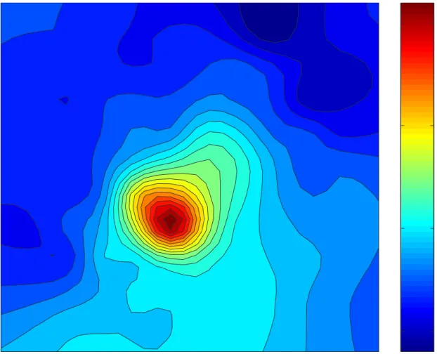
b(κk) which controls the amount of shrinkage of the b parameters. Figure 10 displays the posterior mean of the mean response function. There is a rather sharp peak around (0.42,0.4) and the function displays a slow decay in the general south direction with a much sharper decay in all other directions. The function seems much smoother towards the boundary. This is exactly the type of function for which adaptive spatial smoothing can substantially improve the fit.
Figure 11 shows that in large areas of the map σ²(·) is smooth and has very small values. However, in a neighborhood of the peak of the mean function, σ²(·) displays two relatively sharp maxima located N-N-W and S-S-E of the peak. Severe heteroscedasticity can also be noted near the eastern boundary of the map, especially in the N-E and S-E. Another area displaying heteroscedasticity is the S-W corner of the map. To check whether these characteristics of the function are present in the data we also performed a two-stage frequentist analysis. In the first stage we used a low rank thin plate spline for the
mean function and the results from this regression were used to obtain residuals. We then fitted another low rank thin plate spline to the absolute values of these residuals. While this map was not identical to the one in Figure 11, it did exhibit the same patterns of heteroscedasticity.
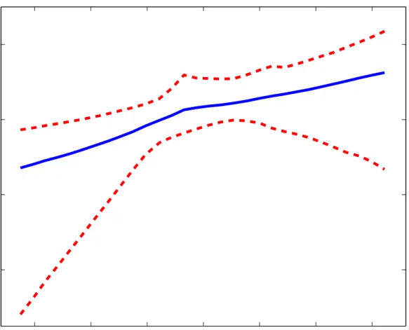
The process log{σ2
b(κk)} controlling the shrinkage of the bk is displayed in Figure 12. Smaller values of this function correspond to less shrinkage of bk towards zero and more local behavior of the smoother. Figure 12 indicates that in a neighborhood of the peak of the mean function the shrinkage is smaller to allow the mean function to change rapidly. Away from the peak, the shrinkage is larger corresponding to a smoother mean. If a fixed smoothing parameter were used, then the representation of its posterior mean in Figure 12 would be the hyperplane Z =−4.71.
To provide a better understanding of the results we posted 4 movies on the website www.people.cornell.edu/pages/cmc59/moviefiles/. The first 3 movies show the poste-rior mean of the mean, standard deviation and shrinkage functions. The 4th movie displays various realizations from the posterior distribution of the mean function.
9
Comparisons with other adaptive surface fitting
meth-ods
Lang and Brezger (2004) compared their adaptive surface smoothing method with several methods used in a simulation study by Smith and Kohn, 1997: MARS (Friedman, 1991), “locfit” (Cleveland and Grosse, 1991), “tps” (bivariate cubic thin plate splines with a sin-gle smoothing parameter), tensor product cubic smoothing splines with five smoothing pa-rameters, and a parametric linear interaction model. We will use the following regression functions, also used by Lang and Brezger
• f1(x1, x2) = x1sin(4πx2) where x1 and x2 are distributed independently uniform on [0,1].
• f2(x1, x2) = 1/5 exp(−8x12) + 3/5 exp(−8x22) wherex1 and x2 are distributed indepen-dently normal with mean 0.5 and variance 0.1.
Function f1(·) correspond to models with interactions and f2(·) has only main effects. Function f1(·) has moderate spatial variability, while function f2(·) is much smoother. We used a sample size n = 300,σ = 1/4range(f) and 250 simulations from each model.
Our model is more general than the models considered by Lang and Brezger (2004) because it incorporates simultaneous nonparametric estimation of the error variance. To assess the performance of the spatially adaptive component of our model we modeled the mean function as a low rank thin–plate spline with an equally–spaced 12×12 knot grid. We
modeled the smoothing parameter using a low rank log-thin plate spline with an equally–
spaced 5 ×5 knot grid. We considered two estimators, one with constant error variance
(CEV) and one with estimated error variance using a log–thin plate spline (EEV) with the
same 12 × 12 knot grid as for the mean function. and a constant error variance. The
CEV estimator is the one that can directly be compared with the estimators considered by Lang and Brezger (2004). One expects that the CEV outperforms the EEV estimator when the true mean error process is homoscedastic and is outperformed by EEV when it is heteroscedastic. We investigate this in our simulations and we compare the performance of our estimators with the performance of estimators considered by Lang and Brezger (2004).
The performance of all estimators was measured by the empirical mean squared error given by MSE( ˆf) = 1/nPni=1{f(xi)−fˆ(xi)}2 and we compared log(MSE) for our method with the values reported by Lang and Brezger (2004).
For the CEV estimator and functionf1(·) corresponding to moderate spatial heterogene-ity we obtained a median log(MSE) of −3.67 with an interquartile range [−3.80,−3.53] and a range [−4.21,−3.13]. These values are better than the ones reported by Lang and Brezger’s methods in their Figure 5–b) and are also better than all the other methods considered in the comparative study of Lang and Brezger. Remarkably, the EEV estimator performed almost as well as the CEV estimator in this case and outperformed all the other
meth-ods considered. The median log(MSE) for EEV was of −3.59 with an interquartile range
[−3.74,−3.43] and a range [−4.14,−3.02]. These results are consistent with univariate re-sults reported by Ruppert and Carroll (2000), Baladandayuthapani, Mallick and Carroll (2004) and Lang and Brezger (2004) who found that allowing the smoothing parameter to vary smoothly outperforms other adaptive techniques when the function requires adaptive smoothing.
For functionf1(·) figure 13 displays the coverage probabilities for the 95% credible inter-vals calculated over a 20×20 equally spaced grid in [0,1]2. For one grid point we calculated the frequency with which the 95% pointwise credible interval covers the true value of the function at the grid point. As expected, these coverage probabilities show strong spatial correlation with lower coverage probabilities along the ridges of the sinus function. Coverage probability is lowest when x1 is in the [0.2,0.5] range. The signal–to–noise in this region is about half the signal–to–noise ratio in the region corresponding to x1 close to 1. This explains why the coverage probability is smaller in this region. Another region with high coverage probability isx1 <0.15 which corresponds to high degree of attenuation of the sinus function. Interestingly, the zeros of the true function appearing at x2 = 0.25, 0.50, 0.75 are covered with at least 95% probability. Another interesting feature is the lower coverage probabilities near the north, south and east boundaries. These features of the pointwise cov-erage probability map are not consistent with the covcov-erage probabilities reported by Lang and Brezger for their Bayesian P–spline method.
For our CEV estimator and functionf2(·) corresponding to very low spatial heterogeneity we obtained a median log(MSE) of −5.95 with an interquartile range [−6.12,−5.66] and a range [−6.51,−5.41]. We compare this results with the results reported by Lang and Brezger in their Figure 5–a). In this case our method performs roughly similar to the Bayesian P–spline method of Lang and Brezger and to the cubic thin plate spline (tps), being outperformed only by Lang and Brezger’s adaptive P–spline method with two main effects. We could also add two main effects to our bivariate adaptive smoother to improve MSE for this example, but this is not our concern in this paper. Again, the EEV estimator performed very similarly to our CEV estimator.
The last simulation study was done using the functionf1(·,·) wherex1,x2are independent uniformly distributed in [0,1] with an error standard deviation function
σ²(x1, x2) = r 32 + 3r 32x 2 1 ,
wherer= range(f1). We compared our CEV and EEV estimators described at the beginning of this section and, as expected, the EEV estimator outperformed the CEV both in term on log(MSE) and coverage probabilities. More precisely for log(MSE) we obtained a median of −5.26 for CEV and −5.35 for EEV, an interquartile range [−5.37,−5.15] for CEV and [−5.48,−5.24] for EEV, and a range [−4.65,−5.72] for CEV and [−4.84,−5.84] for EEV. For both estimators the general patterns for coverage probabilities were the ones displayed in Figure 13. EEV outperformed CEV in terms of coverage probabilities. For example, the regions where the nominal level is exceeded for both estimators have a roughly similar shape and location, but the EEV coverage probabilities tend to be closer to their nominal level.
The simulation studies reported here required more than 2,000 hours of computation time.
10
Implementation using MCMC
We will now provide some details for MCMC simulations of model (1), where the variances σ2
²(xi) and σb2(κk) are modeled by equations (3) and (4). The implementation for other models, e.g., for the multivariate smoothing in Section 7, is similar. Consider independent normal priors for the coefficients of the monomials: βi ∼ N(0, σ0,β2 ), γi ∼ N(0, σ0,γ2 ), i = 0, . . . , p, δi ∼N(0, σ20,δ), i= 0, . . . , q,and independent inverse Gamma priors for the variance components: σ2
c ∼ IGamma(ac, bc) and σd2 ∼ IGamma(ad, bd). Using these priors many full conditionals of the posterior distribution are easy to derive, while a few have complex mul-tivariate forms. Our implementation of the MCMC using mulmul-tivariate Metropolis-Hastings steps proved to be unstable with poor mixing properties. A simple and reliable solution was to change the model by adding error terms to the log-spline models, that is
½ log{σ2 ²(xi)} = γ0+. . .+γpxpi + PK² s=1cs(xi−κ²s)p++ui log{σ2 b(κmk)} = δ0+. . .+δq(κmk)q+ PKb s=1ds(κmk −κbs)q++vk , (12)
where ui ∼N(0, σu2) andvk∼N(0, σ2v). This idea was also used for σb2 by Baladandayutha-pani, Mallick, and Carroll (2004). We fixed the values of σ2
u =σv2 = 0.01, as these variances appear not identifiable or only weakly identifiable and a standard deviation of 0.1 is small on a log-scale. This device reduces the computational costs because one can now use univariate MH steps to simulate from complex full conditionals.
Define as before byΣ²,Σb,θX, and defineθ² = (γT,cT)T,θb = (δT,dT)T,CX = (X Z), C² = (X² Z²), Cb = (Xb Zb), where X, X², Xb contain the monomials and Z, Z², Zb contain the truncated polynomials of the spline models for m, log{σ²2}, and log{σb2}. respectively. Also, denote by
Σ0X = · σ2 0,βIp+1 0 0 Σb ¸ Σ0²= · σ2 0,γIp+1 0 0 σ2 cIK² ¸ Σ0b = · σ2 0,δIq+1 0 0 σ2 dIKm ¸ . The full conditionals of the posterior are detailed below
1. [θX]∼N ¡ MXCTXΣ−²1Y,MX ¢ ,where MX = ¡ CTXΣ−²1CX +Σ−0X1 ¢−1 . 2. [θ²] ∼ N ¡ M²CT²Y²/σ2u,M² ¢
, where Y² = [log(σ2²,1), . . . ,log(σ²,n2 )]T and M² = (CT²C²/σ2u +Σ−0²1)−1. 3. [θb]∼N ¡ MbCTbYb/σv2,Mb ¢ whereYb = £ log(σ2 1), . . . ,log(σK2m) ¤T andMb = (CTbCb/σv2 +Σ−1 0b )−1. 4. [σ2 c]∼IGamma (ac+K²/2, bc+||c||2/2). 5. [σ2 d]∼IGamma (ad+Kb/2, bd+||d||2/2). 6. [σ2
²,i] ∝ σ−²,i3exp n −(yi−µi)2/(2σ²,i2 )− £ log(σ2 ²,i)−ηi) ¤2 /(2σ2 u) o
, where µi and ηi are the ith components of CXθX and C²θ² respectively.
7. [σ2 k] ∝ σ−k3exp n −b2 k/(2σk2)−[log(σk2)−ζk)]2/(σ2v) o
, where ζk is the kth component of Cbθb.
All the above conditionals have an explicit form with the exception of the n+Km
one-dimensional conditionals from 6. and 7. For these distributions we use the
Metropolis-Hastings algorithm with a normal proposal distribution centered at the current value and small variance.
An appealing feature of our methodology is that it can be implemented in high-level Bayesian software such as WinBUGS. Simulations implemented in WinBUGS and MATLAB gave similar results. However, in the simulation study in Section 6 WinBUGS produced credi-ble intervals with lower coverage probability. This is probably due to its sampling inefficiency when parameters are very highly correlated. Programs for our two examples are available
the full model for both our univariate examples, we obtained more than 100 simulations per second from the target distribution (3.4GHz CPU, 3.4Gb RAM PC). We discarded the first 20,000 burn-in simulations and used 100,000 additional simulations from the target distribu-tion for our inferences. For one model and one data set this took approximately 20 minutes of computation time. For the Noshiro example with a full model we obtained approximately 3 simulations per second. we discarded the first 4,000 simulations and used 10,000 additional simulations from the target distribution for our inference. This took approximately 3 hours of computation time.
In complex models the amount of simulation needed for accurate estimation of the pos-terior depends on the parameters monitored. In the LIDAR case, accurate inference for the parameters modeling log{σ2
b(·)} requires tens of millions of simulations whereas the mean function only requires several thousand simulations. This seems due to some parameters be-ing highly correlated or only very weakly identified from the data. Another issue is possible multimodality of the posterior. In a few very long runs we have noted that parameters in log(σ2
b) tend to shift between 2–3 mean levels, suggesting the need for longer runs if these are more than nuisance parameters. Fortunately, the estimates and credible intervals for m(x) do not change much with these changes in log(σ2
b).
Acknowledgements
Carroll’s research was supported by a grant from the National Cancer Institute (CA-57030) and by the Texas A&M Center for Environmental and Rural Health via a grant from the National Institute of Environmental Health Sciences (P30-ES09106).
References
Baladandayuthapani, V., Mallick, B.K., and Carroll, R.J. (2004). Spatially Adaptive Bayesian Regression Splines, J. of Comp. and Graph. Statist., to appear.
Brumback, B., Ruppert, D. and Wand, M.P., (1999). Comment on Variable selection and function estimation in additive nonparametric regression using data-based prior by Shively, Kohn, and Wood. J. Am. Statist. Assoc., 94, 794–797.
Carroll, R.J. (2003). Variances are not always nuisance parameters: The 2002 R. A. Fisher Lecture. Biometrics, 59, 211–220.
Carroll, R.J. and Ruppert, D. (1988). Transformation and Weighting in Regression. New York: Chapman and Hall.
Crainiceanu, C. and Ruppert, D. (2004). Likelihood ratio tests in linear mixed models with one variance component. J.R. Statist. Soc. – Series B, 66(1), 165–185.
Crainiceanu, C.M., Ruppert, D., and Wand, M.P. (2004). Bayesian analysis for penalized spline regression using WinBUGS, submitted.
Eilers, P.H.C. and Marx, B.D. (1996). Flexible smoothing with B–plines and penalties (with discussion). Statist. Sci., 11, 89–121.
Eilers, P.H.C. and Marx, B.D. (2004). Splines, Knots, and Penalties. Manuscript.
Friedman, J.H. (1991). Multivariate adaptive regression splines (with discussion). Ann. Statist., 19, 1–141.
Gelman, A. (2004). Prior distributions for variance parameters in hierarchical models, manuscript.
Gray, R.J. (1994). Spline-based tests in survival analysis. Biometrics, 50, 640–652.
H¨ardle, W. (1990), Applied Nonparametric Regression. Cambridge University Press, New York.
Holst, U., H¨ossjer, O., Bj¨orklund, C., Ragnarson, P. and Edner, H. (1996). Locally Weighted Least Squares Kernel Regression and Statistical Evaluation of LIDAR mea-surements, Environmetrics, 7, 401–416.
Kammann, E.E. and Wand, M.P. (2003). Geoadditive models. Appl. Statist., 52, 1–18. Kauermann, G. (2002). A note on bandwidth selection for penalised spline smoothing.
Technical Report 02-13, Department of Statistics, University of Glasgow
Lang, S., and Bretzger, A. (2004). Bayesian P-splines. J. of Comp. and Graph. Statis., 13, 183–212.
Lang, S., Fronk, E.M. and Fahrmeir, L. (2004). Function estimation with locally adaptive dynamic models, to appear.
Natarajan, R., and Kass, R.E. (2000), Reference Bayesian methods for generalized linear mixed models, J. of the Amer. Statist. Assoc., 95, 227-237.
Ngo, L. and Wand, M.P., (2004). Smoothing with mixed model software, J. Statist. Soft-ware, 9.
Nychka, D., Haaland, P., O’Connell, M., and Ellner, S. (1998). FUNFITS, data analysis and statistical tools for estimating functions. In D. Nychka, W.W. Piegorsch and L.H. Cox (Eds.) Case studies in Environmental Statistics (Lecture Notes in Statistics, vol. 132), pp. 159–179. New York: Springer Verlag.
http://www.cgd.ucar.edu/stats/Software/Funfits/
Nychka, D., and Saltzman, N. (1998). Design of air quality monitoring networks. In D. Nychka, W.W. Piegorsch and L.H. Cox (Eds.) Case studies in Environmental Statistics
Ruppert, D. (1997). Local polynomial regression and its applications in environmental statistics, In Statistics for the Environment, Volume 3, Barnett, V., and Turkman, F., ed., pp. 155–173, Chicester: John Wiley.
Ruppert, D., (2002). Selecting the number of knots for penalized splines. J. of Comp. and Graph. Statis., 11, 735–757.
Ruppert, D. and Carroll, R.J., (2000). Spatially-adaptive penalties for spline fitting. Aust. and New Zeal. J. of Statistics, 42(2), 205–223
Ruppert, D., Wand, M.P., and Carroll, R.J. (2003) Semiparametric Regression. Cambridge University Press, Cambridge.
Sigrist, M. (ed.), (1994). Air Monitoring by Spectroscopic Techniques (Chemical Analysis Series, Vol. 127), Wiley, New York.
Silverman, B.W. (1985). Some aspects of the spline smoothing approach to non–parametric regression curve fitting, J.R. Statist. Soc. – Series B, 47(1), 1–52.
Smith, M. and Kohn, R. (1997). A Bayesian Approach to Nonparametric Bivariate Regres-sion. J. Am. Statist. Assoc., 92, 1522–1535.
Wand, M.P. (2000). A comparison of regression spline smoothing procedures. Comp.
10 15 20 25 30 35 40 0 1 2 3 4 5 6 7 number of knots MASE
equal, not adaptive
equal, adaptive
quantile, not adaptive quantile, adaptive
Figure 1: MASE for non-Bayesian estimators with non-adaptive penalties and equal (EM) or quantile (QS) knot spacings. MASE is based on 1000 simulations from the model
Yi = 10 sin{60xi/(1 + 3xi)} +²i with ²i ∼ N(0,9) where the covariate values are xi = (i−1/99)4, i = 1, . . . ,100. The number of knots was varied and equalled 10, 15, 20, 30, and 40.
400 500 600 700 −1 −0.8 −0.6 −0.4 −0.2 0 Gamma(10−10,10−10) 400 500 600 700 −1 −0.8 −0.6 −0.4 −0.2 0 Gamma(10−6,10−6) 400 500 600 700 −1 −0.8 −0.6 −0.4 −0.2 0 Gamma(10−3,10−3) 400 500 600 700 −1 −0.8 −0.6 −0.4 −0.2 0 Gamma(10−1,10−1)
Figure 2: LIDAR data with unstandardized covariate: effect of four mean–one Gamma priors for the precision of the truncated polynomial parameters. The variances of these priors are 10, 103, 106, and 1010 respectively.
400 500 600 700 −1 −0.8 −0.6 −0.4 −0.2 0 Gamma(10−13,10−7) 400 500 600 700 −1 −0.8 −0.6 −0.4 −0.2 0 Gamma(10−15,10−9) 400 500 600 700 −1 −0.8 −0.6 −0.4 −0.2 0 Gamma(10−18,10−12) 400 500 600 700 −1 −0.8 −0.6 −0.4 −0.2 0 Gamma(10−22,10−16)
Figure 3: LIDAR data with unstandardized covariate: effect of four Gamma priors with mean 10−6 for the precision of the truncated polynomial parameters. The variances of these
ho−ho ho−he he−ho he−he 1 2 3 4 5 6 7 8 9 10 x 10−3
Average Mean Square Error
Figure 4: Mean Square Error based on 500 simulations from the models described in Section 6. The mean function was the same for each simulation study. The labels describe the combination of methods used for simulation and inference. For example, “ho–he” corresponds to homoscedastic errors for the simulation model and heteroscedastic errors used for the estimation model. Only the first and the last two boxplots are comparable because they correspond to the same model used for simulations.