The Bootstrap Estimation In Time Series

(1)

Michigan Technological University Michigan Technological University

Digital Commons @ Michigan Tech

Dissertations, Master's Theses and Master's Reports

2015

The Bootstrap Estimation In Time Series

Yun Liu

Michigan Technological University, [email protected]

Liu, Yun, "The Bootstrap Estimation In Time Series", Open Access Master's Report, Michigan Technological University, 2015.

https://digitalcommons.mtu.edu/etdr/40

(2)

THE BOOTSTRAP ESTIMATION IN TIME SERIES

By Yun Liu

A REPORT

Submitted in partial fulfillment of the requirements for the degree of MASTER OF SCIENCE

In Mathematical Sciences

MICHIGAN TECHNOLOGICAL UNIVERSITY 2015

(3)

(4)

This report has been approved in partial fulfillment of the requirements for the Degree of MASTER OF SCIENCE in Mathematical Sciences.

Department of Mathematical Sciences

Report Advisor: Dr. Yeonwoo Rho

Committee Member: Dr. Latika Lagalo

Committee Member: Dr. Seokwoo Choi

Committee Member: Dr. Min Wang

(5)

(6)

List of Figures

3.1 Moving Block Bootstrap . . . 35 3.2 Non-overlapping Block Bootstrap . . . 37 3.3 Circular Block Bootstrap . . . 41

(11)

(12)

List of Tables

4.1 Andrews Simulation Results . . . 71

4.2 AR(1) Simulation Results . . . 72

4.3 MA(1) Simulation Results . . . 73

4.4 AR(1)-SEASON Simulation Results . . . 74

4.5 ARMA(1,1) Simulation Results . . . 75

5.1 Optimal Expected Block Length . . . 89

(13)

(14)

Abstract

Time series, a special case in dependent data sequence, is widely used in many fields. In time series, linear process models are quite popularly used. General form of linear process indicates the time dependence property of time series, AR(p), MA(q) and ARMA(p, q) models are all linear process models. In this report, simulations are based on the simplest models of these linear process models, such as AR(1), MA(1) and ARMA(1,1) models. AR(1)-SEASON, which is developed based on AR(1) model by changing the weight of residuals, is also considered in this report.

To deal with dependent data sequence, common methods which aim to deal with independent data are no longer accurate to do inference. For dependent data, a conventional method involves consistent estimation of the long run variance, for ex-ample, Andrews [2]. However, in Andrews method, it might be hard to determine the bandwidth. As an alternative, bootstrap methods can be used to approximate the limiting distribution. Block based bootstrap methods, such as moving block boot-strap, non-overlapping block bootstrap and circular block bootboot-strap, can be used for dependent data. Stationary bootstrap, which is with flexible block length following

(15)

a geometric distribution with parameter pS, has also been proved to be consistent.

AR-Sieve bootstrap aims to construct a fitted model of AR(ˆp) and resampling the data with the fitted model. In our simulations, we compare finite sample confidence interval coverage rates. We also consider these bootstrap methods with Andrews es-timation of variance [2] and simulations results show that with the help of Andrews estimation, the estimations are more accurate.

A further discussion of determining an optimal block length for AR(1) model is also mentioned in our report.

(16)

Chapter 1 Introduction

The development of statistics is pretty quick along with social and technological development. At the beginning of statistical research, many of theorems are introduced based on i.i.d. data series. However, with the wide use of statistical methods in many other fields, e.g. economics, finance and other fields, i.i.d. data series can no longer satisfy researchers requirements. Then, more theorems came up to deal with dependent data series. A special kind of dependent data series is time series, in which data are dependent with respect to time. One of the popular methods of time series is linear process, some of these linear proces are listed in Chapter 2, which are AR(p), MA(q) abd ARMA(p, q). In the simulations in

(17)

Chapter 5, we consider several simplest linear process models with different methods.

Unlike the methods we use to estimate parameters of i.i.d. data series, the variance of dependent data cannot be estimated in a simple form. Andrews (1991) [2] intro-duced a method to estimate the variance of limiting distribution in regression with time-dependent variables. However, in finite samples, the greater time-dependence in each model, the less accurate of Andrews variance estimation is. For example, Andrews method has to determine the bandwidth during estimating, however, even though Andrews had listed some useful guide for the choice of bandwidth, they are suitable ony for a few kinds of data generating processes. Researchers might want to find other methods to do more accurate inference of dependent data infinite samples.

Bootstrap methods aimed to deal with i.i.d. random variables when they were first introduced. Efron (1979) [11] showed that bootstrap was developed from jackknife method to make up the shortage of jackknife method. In most bootstrap methods, two levels of estimations are calculated. Take the estimation of population mean µ

as an example. The lower level is to use the sample mean Xn to estimate µ; the

(18)

mean of new data constructed by original data, to estimate the sample mean Xn

of the original data. Such kind of bootstrap methods for time series were firstly introduced by Carlstein (1986) [9] for univariate time series based on bootstrap methods with i.i.d. data series, also known as non-overlapping block bootstrap method. In non-overlapping block bootstrap, original data are divided into several blocks, and correlation of data is maintained within blocks, and independence is assumed between blocks. The introduction of non-overlapping block bootstrap methods helped a lot for dependent series, especially time series. However, with different determination of block length in non-overlapping block bootstrap method, the last few observations may not be used into calculation, and this shortage would influence the result somehow. In 1989 [16], moving block bootstrap was introduced to make up the shortage of non-overlapping block bootstrap method. With moving block bootstrap, the starting observation in each block is the second observation in the previous block. And generating of blocks will stop once the last observation is contained into the last block. Therefore, all of the observations are considered into calculation. At the same time, some parts of original data will be calculated more than once, and several beginning and ending observations will be only counted once. In 1994, Politis and Romano came up with circular bootstrap method [20], in which the series was wrapped into a circle. All observations will be counted more

(19)

than once, and if the total number of original data is n, there will be n blocks. These three block bootstrap methods are based on a fixed block length to divide the original data into blocks. Another kind of block bootstrap, also known as stationary bootstrap, divides the original data into blocks with block length following a geometric distribution with parameterp. With non-fixed block length, results shown in Chapter 4 indicates the accuracy of stationary bootstrap, even though with large correlation, stationary bootstrap may not be as accurate as expected. With the development of bootstrap based on dependent data series, another kind of bootstrap was introduced. AR-Sieve bootstrap method is based on the reconstruction of fitted model based on original data. Instead of dividing the original data into blocks and then calculating estimations by using block bootstrap methods, AR-Sieve bootstrap constructs new a series based on the fitted model of original data, and with the new series, AR-Sieve bootstrap calculates the estimations. In practice, we usually cannot get the model and then do calculations. In this paper, simulations of bootstraps are based on the given models, and data series can be generated as the original data from the given model. We use aforementioned bootstrap methods and the Andrews method to construct confidence intervals of µ, and compare average converage rrates. If average converage rate is closer to the nominal level 95%, it means that this method delivers more accurate cofidence interval in finite samples. We also

(20)

consider the average length of confidence interval. The smaller the confidence interval, the more precise the estimation is.

As we mentioned above, original data series is divided into blocks in block bootstrap methods. We consider a simpler but not necessarily the optimal way to calculate the block length and to construct blocks. However, more optional block length is given in Chapter 5 with circular block bootstrap and stationary bootstrap methods, as introduced by Politis and White (2004) [14]. Further, we calculate the theoretical optimal block length of circular block bootstrap and theoretical optimal expected block length of stationary bootstrap for our simulation models in Chapter 4. Even though Politis and White (2004) [14] gave the estimation of block length for these two bootstrap methods, since we only consider most basic models in this paper, then the estimation of block length did not significantly improve the results. With new block length in circular block bootstrap and new parameter p in stationary bootstrap, we choose to do simulations for AR(1) and ARMA(1,1). Results and detailed comparisons are also shown in Chapter 5.

(21)

compare the bootstrap methods with different basic models of time series. Further work can be done with more compicated models, or with other bootstrap methods. Bootstrap methods based on time series are still developing. More methods can be dedicated into dealing with dependent data, and we will continue to work on this.

(22)

Chapter 2 Time Series

In the development of Statistics, many statistical methods related to independent or uncorrelated data, were introduced by scientists to deal with analyzing the natural facts from collecting data. However, in many practical situations, collected data are correlated. In some cases, data are related among themselves; and in other cases, data are collected over time. We name the data collected sequentially in time as

time series. Time series are widely used in economics, quantitative finance, meteo-rology and so on. Researchers might find out the trend of some observations with respect to time. Often, these observations are not independent in most cases, there-fore, it is natural to think about methods that are appropriate for time series analysis.

(23)

Denote the real valued observations in times as · · · , X−2, X−1, X0, X1, X2,· · ·, the

time series is denoted as {Xt}. The random variables are indexed by all integers Z.

The most simple problem in time series is to estimate the population mean µ. Due to the time dependence, we generally need to use different methods. In the rest of this chapter, we introduce some basic concepts of time series, including stationarity, models based on stationarity and Andrews(1991) [2] methods to estimate the longrun variance of dependent data.

2.1 Stationary Processes

To deal with the time dependence, we often make assumptions on the form of the time dependence to make the analysis easier. The typical assumption in time series analysis is stationarity. For example, the mean or variance, does not change over time for stationary time series. Two definitions of stationarity are usually applied, strict stationarity and second order stationarity/weak stationarity.[25]

(24)

(Xt1, Xt2,· · · , Xtl)and(Xt1+p, Xt2+p,· · · , Xtl+p)have the same distribution, then the time series Xt is lth- order stationary and it is said to be strictly stationary.

Most of the time, the strict stationarity is too strong to be satisfied. Thus, an alternative definition comes up and it might be easier to work under this as-sumption. In the weak stationarity, the first moment and autocovariance do not change over time in stead of having the same distribution for (Xt1, Xt2,· · · , Xtl) and

(Xt1+p, Xt2+p,· · ·, Xtl+p).

Definition 2.1.2 If, for all integer t and l, the mean of the time series {Xt} is

constant, and if the covariance of Xt and Xt+l only depends on the magnitude of

l, the time series {Xt} is said to be second order stationary, or weak stationary.In

other words, the time series {Xt} is second order stationary, or weak stationary if

E(Xt) =µ and cov(Xt, Xt+l) =γl where µ is a constant and γl is independent of t.

{γl} with integersl is called the autocovariance function at lag l. And we also define

autocorrelation function of Xt at lag l as

ρl=

γl

γ0

=corr(Xt, Xt+l).

(25)

1. Autocoraviance has properties:

γ0 =V ar(Xt), γl =γ−l, |γl| ≤γ0.

2. The strict stationarity does not necessarily mean weak stationarity. However, if we further assume finite second moment, i.e., E|X2

t| < ∞, then all strictly

stationary series are also second order stationary.

3. If the strict stationarity is satisfied while the second moment is infinite, then the second order stationarity can not be implied.

4. The only case where the weak stationarity implies the strict stationary is a weakly stationary Gaussian time series.

(26)

2.2 Models Based on Stationarity

2.2.1 Linear Processes

One of the most popular methods to model the time dependence is to express the variable as a linear combination of an i.i.d. sequence. Let{t}be a sequence of

iden-tically distributed independent random variables with mean zero. A linear process

{Xt}, t∈Z is defined as Xt = ∞ X i=−∞ ψit−i. (2.1) If P∞

i=1ψi2 is infinite, then the variance of Xt will be infinite. Therefore, it is

rea-sonable to assume that P∞

i=1ψ 2

i <∞. Models mentioned below are special cases of

(27)

2.2.1.1 Moving Average Processes

Based on the linear processes expression in 2.1, if only a finite number of ψi are

nonzero, then we can get a moving average process,

Xt= q

X

i=0

θit−i, (2.2)

whereθiare fixed constants,θ0 = 1, constantqindicates the finite number of nonzero

θi, and white noise {t} is a sequence of independent random variables with mean

zero and variance σ2_{. (2.2) is called the} _{moving average process} _{of order} _q_{, denoted}

as MA(q). MA(1) and MA(q) are stationary for every finiteθor every finite sequence

{θi}, i= 1,2,· · · , q. Since according to 2.2, E(Xt) = 0, V ar(Xt) = σ2 q X i=0 θ2_i, γt−i =E(XtXt−i) =E( q X i=0 θit−iXt−i) =        σ2 Pq i=0θiθi+|l| , for |l| ≤q 0, otherwise. .

(28)

Then the sum is finite when every θ is finite. And γt−i does not depend on t, i.e.,

MA(1) and MA(q) are stationary.

In a similar way, we can show that MA(∞) is stationary if the coefficients are abso-lutely summable, i.e., P∞

i=0|θi|<∞.

2.2.1.2 Autoregressive Processes

The autoregressive process of order p, AR(p), can be defined by

Xt−t= p

X

i=1

φiXt−i, (2.3)

where t is a independent random variables sequence with mean zero and variance

σ2, and φi are fixed constants. AR(1) process can be defined as

(29)

In fact, AR(1) can be proved as the second order stationarity. To prove it, we firstly rewrite the definition function of Xt as

Xt−t =φ1(t−1+φ(t−2+φ1(t−3+· · ·))) =φ1t−1 +φ21t−2+φ31t−3+· · · , Xt = t−1 X i=0 φi₁t−i.

Therefore, since t is an independent sequence, from the “new” definition function

we can figure out that AR(1) is a linear process with the mean of Xt being 0, and

the autocovariance function being as follow:

γ0 =E(Xt2 −E(Xt)2) = E(Xt2) =E ∞ X i=0 φi₁t−i !2 =E ∞ X i=0 φ2₁i2_t−i ! =σ2 ∞ X i=0 φ2₁i ! =σ2 1 1−φ2 1 , γl =E(XtXt+l) = E ∞ X i=0 φi₁t−i ∞ X j=0 φj₁t−j+l ! =σ2 φ l 1 1−φ2 1 .

Note that not all AR(p) process is stationary. For example, if φ1 = 1 for AR(1)

(30)

that in AR(p) process is stationary, we do the followings.

Since in AR(p) model, Xt and Xt−1 are related. Back-shift operatorB is defined as

BXt =Xt−1 and BkXt=Xt−k for all k,

then AR(p) can be rewritten with back-shift operator as

Xt= p X i=1 φiXt−i+t = p X i=1 φiBiXt+t. (2.4)

Some operations can be applied on 2.4 to calculate the conditions of φi’s.

Xt− p X i=1 φiXt−i =t (1− p X i=1 φiBi)Xt=t. Denote 1−Pp

i=1φiBi as Φ(B) which is named as autoregressive polynomial of Xt,

then

Φ(B)Xt=t

(31)

Calculate moments of Xt,

E(Xt) = Φ(B)−1E(t) = 0, (2.5)

V ar(Xt) = Φ(B)−2V ar(t)>0. (2.6)

From 2.5, Φ(B) 6= 0. From 2.6, Φ(B)−2 > 0, where Φ(B)−2 = 1/(Φ(B)2). So, Φ(B)2 _>₀

By using the fundamental theorem of algebra, characteristic function Φ(z) can be factored as Φ(z) = p Y i=1 (1− z ri ),

wherer1,· · · , rp ∈Cis the roots of Φ(z) and Cis complex number set. Then AR(p)

is stationary and ergodic if and only if|ri|>1 for alliwhere|ri|is the modulus ofri.

2.2.1.3 ARMA Processes

Another common process belong to the linear processes is the autoregressive moving average process of orders p and q, denoted as ARMA(p, q), where it’s time depen-dence is modeled using an autoregressive representation as well as moving average

(32)

representation. To define ARMA(p, q), we define the function as Xt= p X i=1 φiXt−i+ q X j=0 θjt−j.

Treat the sum of residuals as a whole part, then ARMA(p, q) can be written as the form of AR(p) model. Then it is a linear process with calculation.

Consider the special case, ARMA(1,1), the defining equation can be written as

Xt=φ1Xt−1+t−θ1t−1. (2.7)

The condition of stationarity for ARMA(p, q) is the same as the condition of AR(p) model, i.e., all roots ri’s of Φ(B) = 0 lie outside the unit circle, |ri|>1.

2.2.2 α

-Mixing Processes

Another well known process is α-mixing process. If the process is stochastic, “mix-ing” represents the dependence betweenXt1 andXt2 approaches to zero when|t1−t2|

is increasing, or means “asymptotically independent”.

Consider the probability space, (Ω,F, P), and let F_ij, −∞ ≤ i ≤ j ≤ ∞ be the

(33)

dependence coefficient for any positive integer n and given random sequence X is defined as α(n) = sup A∈Fm −∞, B∈Fm∞+n, m∈Z |P(A)P(B)−P(A∩B)|.

Then, a strictly stationary stochastic process {Xt} is said to be α-mixing if

α(n)→0 as n→ ∞.

Remark 2.2.1 ARMA(p, q) is a α-mixing process.

2.3 Conventional Method to Conduct Testing of

Confidence Interval for

µ

After the introduction of the stationary process above, we can consider the estimation of the mean.

Suppose that we are observing process which satisfy

(34)

where{t}is a stationary time series with mean zero and summable covariances, i.e.

P

|γl| is infinite. Our purpose is to looking at the estimation of the mean µ. The

unbiased estimation of the mean, µ, is the sample mean, given as

Xn =

Pn

i=1Xi

n

Consider the variance of Xn, we could easily obtain that

V ar(Xn) = 1 n n X l=−n 1−|l| nγl = 1 n ( γ0+ 2 X 1≤l≤n 1− l nγl ) .

Let σ2_n=V ar(√nXn), then Theorem 7.1.1 in [4] shows that as n→ ∞,

V ar(Xn)→0 if γn→0, and σ_n2 → ∞ X l=−∞ γl if ∞ X l=−∞ |γl|<∞.

(35)

Refer to Theorem 27.4 in [3], suppose that Xt is stationary and α-mixing process with α(n) =O(n−5_{) and} _E₍_X t) = 0, E(Xt12)<∞, then V ar(√nXn)→ ∞ X l=−∞ γl =V, √ n(Xn−µ) d − →N(0, V). (2.8)

When estimatingV, Andrews (1991) [2] states that the result ofV equals the spectral density function at λ = 0 multiplied by 2π motivates the use of spectral density function. Therefore, we consider to use the spectral density function to estimate V. Consider the estimator of V as

ˆ V = n n−1 n−1 X l=−n+1 k l Sn ˆ γl= n n−1 2 n−1 X l=1 k l Sn ˆ γl+k(0)ˆγ0 ! , (2.9) ˆ

γl is one of the estimator of γl and ˆγl =

1

n

Pn

t=|l|+1ˆtˆt−l where ˆt = Xt−Xn for

(36)

In 2.9, Sn is a band-width parameter. The class of kernels K , is a set of the

real-valued kernels, k(·), which is given by

K =                k(x)∈[−1,1], x∈R k(x) =k(−x), k(0) = 1, ∀x∈R, R∞ −∞k 2₍_x₎_{dx <}_∞_,

k(x) is continuous at 0 at all but finite other points

               .

According to Parzen (1957) [17] and Andrews (1991) [2] mentioned, we consider the corresponding class of kernel estimators of the spectral density function. Parzen (1957) [17] recommends several kinds of kernels and Andrews (1991) [2] selected five of them. We consider two kernels that are commonly used, Bartlett and Quadratic Spectral kernel. Bartlett: kBT(x) =        1− |x| for |x| ≤1, 0 otherwise, Quadratic Spectral: kQS(x) = 25 12π2_x2 sin(6πx/5) 6πx/5 −cos(6πx/5) . (2.10)

Andrews (1991) [2] presented how to get an original bandwidth parameter. The optimal bandwidth estimators, ˆSn, for Bartlett and Quadratic Spectral kernels, are

(37)

Bartlett: Sˆn = 1.1447(( ˆα(1)n)

1/3

,

Quadratic Spectral: Sˆn = 1.3221(( ˆα(2)n)1/5.

(2.11)

where α(q) is a function of the unknown spectral density function f(·), and ˆα(q) is the estimator.

As for α(q), the function of the spectral density function, for AR(1) model, let ψ be the autoregressive variance parameter, and φ1 be the AR coefficient. Let ˆψ and ˆφ1

be their estimators respectively. Then, as mentioned by Andrews (1991) [2],

ˆ α(1) = 2 ˆψ (1−φˆ1)(1 + ˆφ1) !2 , ˆ α(2) = 2 ˆψ (1−φˆ1)2 !2 . (2.12)

For ARMA(1,1) and MA(1) models, the estimated functions ˆα(q) are not the same as AR(1). Andrews (1991) [2] derived the function for ˆα(1) and ˆα(2) for ARMA(1,1) and MA(1) separately.

In ARMA(1,1), the estimation of ARMA parameter (φ1, θ1) is denoted as ( ˆφ1,θˆ1),

then ˆ α(1) = 2(1 + ˆφ1θˆ1)( ˆφ1+ ˆθ1) (1−φˆ1)(1 + ˆφ1)(1 + ˆθ1)2 !2 , ˆ α(2) = 2(1 + ˆφ1 ˆ θ1)( ˆφ1+ ˆθ1) (1−φˆ1)2(1 + ˆθ1)2 !2 . (2.13)

(38)

(39)

(40)

Chapter 3 Bootstrap Methods

3.1 Jackknife and Bootstrap Methods for i.i.d.

data

3.1.1 Jackknife Method

Before we start to introduce the bootstrap, jackknife method should be introduced first and we can obtain a general idea of how jackknife works. The “delete-one”

(41)

jackknife was first introduced by Quenouille (1949) [24]. Suppose that X1,· · · , Xn

is i.i.d. random sample, let ˆθn be the estimator of θ, for some function fn, ˆθn =

fn(X1,· · · , Xn). Then the definition of the jackknife average is

ˆ

θn,i=fn−1(X1,· · ·, Xi−1, Xi+1,· · · , Xn).

The function denotes a statistic calculated with all sample except one observation. Leaving out each observation at one time from the dataset, the jackknife estimator calculates the estimate and find the average of the replicates.

The jackknife estimator of the bias E(ˆθn)−θ can be obtained as

Bias= n−1 n n X i=1 (ˆθn,i−θˆn).

Set ˆθ∗ = nθˆn − (n − 1)ˆθn,i, i = 1,· · · , n, which is called the ith pseudo value.

Therefore, the jackknife estimator of ˆθn, is given as ¯θ∗ = ˆθn−Bias, which can be

calculated ¯ θ∗ = 1 n n X i=1 ˆ θ∗.

(42)

Remark 3.1.1 Expand E(ˆθn) in powers of n−1 according to the property of Quias, En≡=E(ˆθn) = θ+ ∞ X i=1 ak nk, En−1 ≡=E(ˆθn) = θ+ ∞ X i=1 ak (n−1)k, E(¯θ∗) = nEn−(n−1)En−1 =θ− b n(n−1).

Remark 3.1.2 The jackknife estimator of V ar(ˆθn) is given as

d V ar(ˆθn) = 1 n(n−1) n X i=1 (ˆθ∗−θ¯_n∗) = n−1 n V arg(ˆθn−1).

The jackknife estimator V arg(ˆθn−1) of V ar(ˆθn−1) is always upwards.

Unfortunately, the jackknife estimator of variance fails for many non-sufficiently smooth functions. Take the median as an example. The median of a dataset may be influenced a lot when one observation is left out. Then the calculation of the jackknife estimator of variance will not be accurate enough to describe the original dataset.

(43)

3.1.2 Bootstrap Methods

As we mentioned before, Efron (1981) [12] verified that the bootstrap is more dependable than the jackknife. Here we give a brief introduction of bootstrap methods and some particular bootstrap methods.

Suppose that x = (x1,· · · , xn) is an observed random sample from a distribution

with cdf F(x). If X∗ is selected at random fromx, then

P(X∗ =xi) =

1

n, i= 1,· · · , n.

Resampling generates a random sample X₁∗,· · · , X_n∗ by sampling with replacement fromx. The random variablesX_i∗are i.i.d., uniformly distributed on the setx1,· · ·xn.

The empirical distribution function (ecdf) Fn(x) is an estimator of FX,

Fn(x) = 1 n n X i=1 I{Xi ≤x},

(44)

where I{Xi ≤x}=        1 if Xi ≤x, 0 else,

It can be shown that Fn(x) is a sufficient statistic for F(x) and

supx|Fn(x)−FX| a.s.

−−→0, (3.1)

according to Gilvenko-Cantelli Theorem. Moreover,Fn(x) is the distribution function

of a random variable that is uniformly distributed on the set x1,· · ·, xn. Hence the

empirical cdf Fn is the cdf ofX∗, Fn∗.

Thus in bootstrap, there are two approximations: The ecdf Fn is an approximation

to the cdf FX, which we can treat this estimation as the first or the lower layer; the

ecdf F_n∗ of the bootstrap replicates is an approximation to the ecdf Fn, which can

be treated as the second layer or the higher level. Resampling from the sample x is equivalent to generating random samples from the distribution Fn.

To generate a bootstrap random sample by resampling x, generate n random integers i1,· · ·, in uniformly distributed on 1,· · · , n and select the bootstrap sample

(45)

Suppose θ is the parameter of interest (θ could be a vector), and ˆθ is an estimator of θ. Then the bootstrap estimate of the distribution of ˆθ is obtained as follows.

1. For each bootstrap replicate, indexedb = 1,· · · , B:

(a) Generate sample x∗(b) = x∗₁,· · · , x∗_n by sampling with replacement from the observed sample x1,· · · , xn.

(b) Compute thebth _{replicate ˆ}_θ(b) _{from the} _bth _{bootstrap sample.}

2. The bootstrap estimate of F_θˆ(·) is the empirical distribution of the replicates

ˆ

θ(1),· · · ,θˆ(B).

The bootstrap is applied to estimate the standard error and the bias of an estimator in the following sections.

(46)

The bootstrap estimate of standard error of an estimator ˆθ is the sample standard deviation of the bootstrap replicates ˆθ(1),· · · ,θˆ(B).

ˆ se(ˆθ∗) = v u u t 1 B B X b=1 (ˆθ(b)₋_θ¯ˆ∗₎2 where θ¯ˆ∗ = 1 B PB b=1θˆ(b).

Bootstrap Estimation of Bias

If ˆθ is an unbiased estimator of θ, E[ˆθ] =θ. The bias of an estimator ˆθ for θ is

bias(ˆθ) =E[ˆθ−θ] =E[ˆθ]−θ

The bootstrap estimation of bias uses the bootstrap replicates of ˆθ to estimate the sampling distribution of ˆθ. For the finite populationx= (x1,· · · , xn), the parameter

is ˆθ(x) and there are B independent and identically distributed estimators ˆθ(b)_{. The}

(47)

bootstrap estimate of bias is ˆ bias(ˆθ) =θ¯ˆ∗−θ,ˆ where θ¯ˆ∗ = 1 B PB b=1θˆ

(b)_{, and ˆ}_θ _{= ˆ}_θ₍_x_{) is the estimate computed from the original}

observed sample.

The bootstrap method for i.i.d. data is two estimations. To apply bootstrap meth-ods into dependent data, especially time series, covariance of the dependent data is necessary to consider into different bootstraps since covariance is quite important to describe the dependent data. Therefore, some different bootstrap methods are introduced.

3.2 Bootstrap Methods for Dependent Data

As we mentioned before, the conventional method to estimate the population mean is based on the limiting distribution being standard normal distribution. However, in time series, Andrews method to estimate the variance can not be applied every time. First, Andrews method is based on the selection of bandwidth in the kernel calculation. Even though Andrews listed several selection of bandwidth, it is not enough to cover all kind of models. Selection of bandwidth is a hard thing to be

(48)

determined in Andrews methods. Second, it is known that Andrews method may not deliver accurate size or coverage rates in finite samples. Hereby, we introduce the bootstrap methods to approximate the limiting distribution. The main idea of most bootstraps methods is re-sampling. The most popular bootstrap methods for dependent data, especially time series, are block bootstrap, sieve bootstrap and stationary bootstrap.

3.2.1 Block Bootstraps

Bootstrap methods are aiming to re-sample the data to get the estimator not related on the limiting distribution. However, in normal cases, the bootstrap which was introduced by Efron (1979) [11] is dealing with i.i.d dataset. Bootstrap has been developed by several researchers to explore the fields that it can deal with to make it more useful and developed. The principal ideas of different bootstraps are quite similar, but with different models and procedures. The block bootstraps are introduced to deal with dependent data series, especially time series.

(49)

Instead of resampling the whole dataset which was introduced by Efron (1979) [11], subsamples are randomly captured from the whole series which is divided into several blocks, with block lengthl < nandb blocks, to keep the dependent structure of neighbored observations. Hereby, we introduce two block bootstrap methods.

3.2.1.1 Moving Block Bootstrap

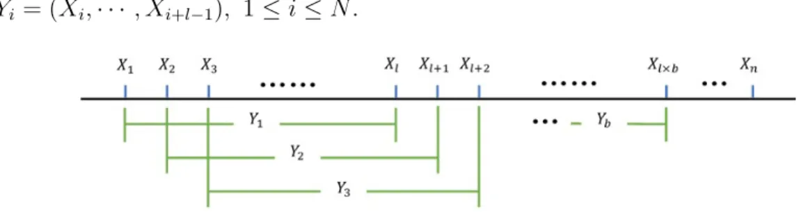
Moving block bootstrap, in short MBB, is one of the popular bootstrap methods in inference of time series. Overlapping block bootstrap was introduced [13] in the same setting. Suppose that the series{Xt}is a sequence of weak stationary variables,

divide the series into several blocks under the condition

l → ∞as n→ ∞ but with l

n →0,

where l is the block length and n is the number of total observations in time series. Under the condition of weak stationary, dependence are kept within each block, and these blocks can be assumed as i.i.d.

(50)

In MBB, after determing the length of blocks,l, we can getN =n−l+ 1 i.i.d blocks

Yi = (Xi,· · · , Xi+l−1), 1≤i≤N.

Figure 3.1: Moving Block Bootstrap

In N i.i.d blocks, we randomly select b = bn/lc blocks, Y₁∗,· · · , Y_b∗, to construct a new series with these selected blocks as {X₁∗,· · · , X_m∗} where m = lb. The total number of the samples in the new series isl×b. With the new series, we can calculate the new sample mean X∗_n in each replicates, denoted by X∗_n(b), and it is easy to get the confidence interval with B replicates.

Theorem 6 in [16] shows the consistency of MBB under some conditions.

Theorem 3.2.1 Suppose that random variables {Xt}, t= 1,· · ·, n construct a

sta-tionary m-dependent sequence with EX1 = µ and E|X1|4+δ < ∞ for some positive

δ. Ifl/n→0 when n → ∞, then sup x |P∗{√m(X∗ m−E∗(X∗m))≤x} −P{ √ n(Xn−µ)≤x}| P −→0, (3.2)

(51)

where P∗ is the bootstrap probability and E∗ is the mean under the bootstrap proba-bility and X∗_m = Pm t=1X ∗ t m .

If the condition l/n →0 can be replaced by l/√n →0 as n → ∞, then E∗X∗

m can

be replaced by X in 3.2.

In Theorem 3.2.1, m-dependence is defined as follows. Let {X1, X2,· · · } be

a sequence with random variables, let A be an event based on the sequence

{X1,· · · , Xh} and B be an event based on {Xh+1+m,· · ·,}. If any pair of events A

and B are independent, then the sequence {Xt} is m-dependent. As Liu and Singh

mentioned in [16], “The notion of m-dependence is probably the most basic model which takes into account such dependence.” The proof of this theorem can be found in [16].

In Theorem 3.2.1, two different cumulative density functions are involved, and two estimations are considered, which can be treated as two different layers. The first estimation or the first layer, is the estimation of population with the given sample, which is expressed as P{√n(Xn−µ) ≤ x}. This is the usual layer we are looking

at without bootstrap. If the limiting distribution is involves nuisance parameters, bootstrap can be used to approximate the limiting distribution of a function of

(52)

given data, for example, the mean. Therefore, the second estimation, or the second layer, which is expressed by P∗{√m(X∗_m − E∗(X∗_m)) ≤ x}, can be generated. Then Theorem 3.2.1 shows that the difference between the two cumulative density functions (one of them is the cdf of bootstrap method, and another one is the cdf of the sample series) convergent to 0 in probability.

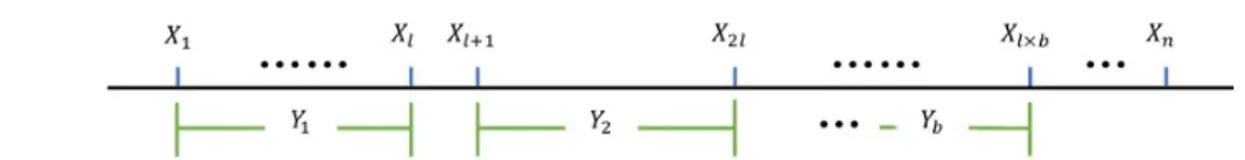
3.2.1.2 Non-overlapping Block Bootstrap

The nonoverlapping block bootstrap, as known as NBB, is firstly introduced by Carlstein in 1986 for univariate time series. [9] NBB and MBB only have several differences on defining the blocks. In MBB, the total number of blocks is n−l+ 1, and the blocks are defined overlapping. However, in NBB, we divide the whole series into approximately independent blocks {Yi}, where Yi = {X(i−1)l+1,· · · , Xil}, i =

1,· · · , b, and then we sample b blocks Y₁∗,· · · , Y_b∗, putting these blocks together to get X₁∗,· · · , X_m∗.

(53)

Since we already showed the consistency of MBB, comparing MBB with NBB, if the difference between MBB and NBB can be insignificant and negligible, then NBB is consistent.

The estimated parameter in bootstrap version in general, can be denoted as θ_bl,n∗ =

T(F_bl,n∗ ), and in special, we are discussing the mean for all of these methods. To separate MBB and NBB, the estimator of MBB in the bootstrap version is denoted as θ∗_bl,n(M), while the estimator of NBB isθ∗_bl,n(N).

θ_bl,n∗(M) = 1 bl bl X j=1 X_j∗(M), and θ∗_bl,n(N) = 1 bl bl X j=1 X_j∗(N).

The probability of selecting any block is N−1_,

P{(X₁∗,· · · , X_l∗) = (Xi,· · · , Xi+l−1)|Xn}

=P{Yj =i|Xn}

=N−1 ,for 1≤i≤N.

(54)

While the probability of selecting any block is b−1_,

P{(X₁∗,· · ·, X_l∗) = (X(i−1)l+1,· · · , Xil)|Xn}

=P{Yj =i|Xn}

=b−1 ,for 1 ≤i≤b.

(3.4)

Hence, from 3.3, we get

E(θ_bl,n∗(M)) = 1 N N X j=1 1 l l X i=1 Xj+i−1 ! = 1 N b l−1 X r=1 r(Xr+XNr+1) +l N X s=l Xs ! = 1 N n X r=1 Xr− 1 l l−1 X s=1 (l−s)(Xs+Xn−s+1) ! . (3.5)

And from 3.4, we get

E(θ∗_bl,n(N)) = 1 b b X j=1 1 l l X i=1 X(j−1)l+i ! = 1 bl n X r=1 Xr− n X i=bl+1 Xi ! . (3.6)

Notice that when the process {Xt} is under some conditions and some standard

(55)

of the squared bias is E(E(θ∗_bl,n(M))−E(θ_bl,n∗(N)))2 ₌_O₍_l/n2_{), that is, for large sample}

size, the difference between these two methods is insignificant and negligible. [15]

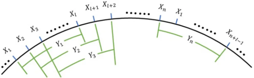
3.2.1.3 Circular Block Bootstrap

Another popular bootstrap method with fixed block length, is circular block bootstrap, also known as CBB. After the introduction NBB and MBB, CBB was firstly introduced by Politis and Romano in 1994 [20], which ’wrap’ the series into a circle, to make fully use of every observation in the series, comparing with NBB. As we can see, in NBB, the last several elements cannot be included in any block when the length of the block is not a divisor of the total number of observations. Then, when we construct bootstrap procedure, these not-included observations are deleted by resampling. However, in CBB, when the series is wrapped like a circle, and there are n blocks, while n−l+ 1 blocks are constructed in MBB. The “wrapped circle” is defined as Xi ≡Xj for i > n, where j =i modn, and X0 =Xn.

As mentioned above, let the series be {X1,· · · , Xn}, then the whole arc of the

“wrapped circle” is {X1,· · · , Xn, X1,· · · , Xn+l−1}, thus, by setting the block length

(56)

block set is {Y1,· · · , Yn}. Sampling with replacement with probability 1/n,

ran-domly select b i.i.d blocks from the set where lb = m ≈ n. Then we have a new series as X₁∗,· · ·, X_m∗. With the new series, the confidence interval can be calculated by following the similar procedure mentioned above, and we can also get the true percentage.

Figure 3.3: Circular Block Bootstrap

The following theorem were stated by Politis, D.N., Romano, J.P. [20] shows the consistency and asymptotic accuracy of CBB. The theorem is aiming to show the consistency of circular block bootstrap with α-mixing series.

Theorem 3.2.2 Let {Xt} be a sequence assumed to be with weak stationarity.

Spe-cially, the α-mixing condition (α(h) → 0 as h → ∞, where α(h) is defined in Chapter 2) is assumed. Assume that E|Xt|6+δ < ∞ for some positive δ, and

(57)

P∞

h=1n2(α(h))

δ

6+δ <∞. As n → ∞, let m/n→1 where m=lb, and let l→ ∞ but

b/n→0. Thenσ2 n ≡V ar( √ nXN)is limiting toσ∞2 <∞, andV ar∗( √ mX∗_m)−→P σ2 ∞, where V ar∗ is the variance of √mX∗_m under the bootstrap probability P∗, and

supx|P∗{ √ m(X∗_m−Xn)≤x} −P{ √ n(Xn−µ)≤x}| p − →0, (3.7)

for almost all sample series {Xt} for t = 1,· · · , n.

The meaning of Theorem 3.2.2 is similar with the Theorem 3.2.1. The theorem shows the consistency of CBB. Since blocks are defined similar in MBB, NBB and CBB, the proofs of consistency of three block bootstraps are quite similar.

3.2.1.4 Stationary Bootstrap

In the previous three methods, the block length is fixed. A new resampling method, which is also generally available and useful for stationary weakly time series, called stationary bootstrap, also known as SB, was introduced by Politis and Romano [21] in 1994. In contrast to the former mentioned block bootstraps, resampling procedure is repeated in stationary bootstrap to get an approximation to the

(58)

distribution of the statistic with generating the pseudo-time series as a stationary time series, i.e. stationary bootstrap aims to retain the stationarity of the original series in resampling. The block is of random length, and the block length can be assigned to have some kind of distribution. Usually, the selected distribution of the block length is a geometric distribution.

Suppose that {Xt} is a given stationary weakly time series as mentioned before.

Define each block as Bi,l = {Xi, Xi+1,· · · , Xi+l−1}, where l is length of the block.

Since when we randomly choose the starting point of each block and the block length has a geometric distribution, then observations in some block may exceed the given sample sequence. To avoid “cutting off” some observation in some blocks, “wrapping” the series may help to keep all observations which should be included in the blocks. Define the “wrap” as Xi ≡Xj for i > n, where j =i( mod n), and

X0 =Xn. Since the block lengths may be different, then definel1, l2,· · · be the block

length independent to Xi, and {li} is a sequence of i.i.d random variables which

have a geometric distribution P{li =u} = (1−pS)u−1pS for u= 1,2,· · ·. Then for

any given pS, we can generate the sequence {li}. As for the index of the starting

point of each blockii independent toXi and li, randomly select from{1,· · · , n}, i.e.

(59)

on {1,· · · , n}. Therefore, the sampled sequence of blocks with random length is

{Bi1,l1, Bi2,l2,· · · } = {Xi1, Xi1+1,· · · , Xi1+l1−1, Xi2, Xi2+1,· · · , Xi2+l2−1,· · · }. If the

sequence length is greater then the sample size n, then stop the process once n

observations are generated. By simulating a large number of pseudo time series, the distribution of T∗ can be approximated, the critical value and confidence interval can be calculated then.

Like the previous theorems mentioned above, the consistency of stationary bootstrap aims to show the difference of two estimations convergent to 0. Theorem 1 in [21] shows the consistency of stationary bootstrap.

Theorem 3.2.3 Assume that {Xt} for t = 1,2,· · · is a strictly stationary process

which the autocovariance γ(·)satisfiesγ(0) +P

r|rγ(r)|<∞. Assume the condition

3.8 holds where κ4(u, v, w) is the fourth joint cumulant of the distribution of

(Xi, Xi+u, Xi+v, Xi+u+v+w).

X

u,v,w

(60)

Assume E|X|2+δ_<_∞ _andP

h[α(h)]

δ

2+δ for some positive δ where α(h)is defined in Chapter 2. Then, σ_∞2 =V ar(X1) + 2 P∞ i=1cov(X1, X1+i) is finite. If σ2 ∞>0, then supx|P{ √ n(Xn−µ)≤x} −Φ(x/σ∞)| →0, (3.9)

where Φ(·) is the standard normal distribution function.

Assume that the lag pS →0 in the geometric distribution and npS → ∞ , then the

bootstrap distribution is close to the true sampling distribution given as

supx|P∗{ √ n(X∗₋_X n)≤x} −P{ √ n(Xn−µ)≤x}| P −→0,

where P∗ is the bootstrap probability mentioned above.

It has to be mentioned that, the form of the convergence in Theorem 3.2.3 is quite similar with the previous theorems only with √n in the first cumulative function instead of m. Since in stationary bootstrap, we stop generating sequence once n

variables are generated, then the total length of the new sequence is the same with the original data. It is possible to getn variables in NBB, MBB or CBB if the block

(61)

length is chosen in some way.

3.2.2 AR-Sieve Bootstrap

AR-sieve bootstrap develops another way. Instead of constructing blocks from the original data, AR-sieve bootstrap aims to establish an AR(ˆp) time series model and construct series based on the model to estimate the parameter. The essentials in AR-sieve bootstrap is to estimate the parameters in AR(ˆp) model and to determine the residuals from the original series in [5], [7], [6].

Let{X1,· · · , Xn}be the original time series. The purpose of AR-sieve approximation

is to construct an AR(ˆp) model

Xt−µ= ˆ p X i=1 φi(Xt−i−µ) +t,

where µ is E(Xt) and t is an innovation sequence independent of {Xs;s < t},

which is of i.i.d random variables with expectation 0. Since we need to estimate the series with an AR(ˆp) model, then the first thing is to determine the order ˆp.

(62)

Usually Akaike information criterion can help to find the autoregressive order ˆp. Let ˆ

φpˆ = ( ˆφ1,n,φˆ2,n,· · · ,φˆp,nˆ ) be the Yule-Walker autoregressive parameter estimators,

then ˆ φpˆ= ˆΓ−_p_ˆ1γˆpˆ, ˆ γk = 1 n n−|k| X t=1 (Xt−Xn)(Xt−|k|−Xn), for 0≤k≤p,ˆ whereXn = Pn t=1Xt n , ˆΓpˆ= ˆγ(|s−r|) for s, r= 1,· · · ,pˆ, and ˆγpˆ= (ˆγ(1),· · ·,γˆ(ˆp)) 0_.

With Yule-Walker estimators, some part of the estimated AR(ˆp) can be determined. Then another important part is the residuals. To keep the information of the original data, let ˆt =Xt−

Ppˆ

i=1φˆiXt−i, i = ˆp+ 1,· · · , n be the residuals of the model fit,

then we can define the empirical distribution function of i.i.d. residuals.

Fˆt(x) = 1 n−pˆ n X t= ˆp+1 I[ˆt−ˆt ≤x], where ˆt= 1 n−pˆ Pn t= ˆp+1ˆt.

(63)

model. The fitted AR(ˆp) model is given as X_t∗−Xn = ˆ p X i=1 ˆ φi(Xt∗−i−Xn) + ˆ∗t, (3.10)

where ˆ∗_t is i.i.d. residuals with marginal distribution Fˆt(x). Since if we set ˆp,

then the first ˆp’s estimated values cannot be calculated according to 3.10, then in order to get a series, it is necessary to set these estimated values. Several ways can help to set these values, for example, set these as 0, or as Xn. Assuming that

Y = f(X1,· · · , Xn) is a function of the original data, then the AR-sieve bootstrap

function can be defined as Y∗ = f(X₁∗,· · · , X_n∗). To show the consistency of sieve bootstrap, Theorem 3.1 in [5] gives a proof for general cases with AR(∞) model. Assume that {Xt} for t ∈ Z is a stationary process with EXt = µ. As what has

been mentioned in [5], according to Wold’s Theorem, if the sequence {Xt} is purely

stochastic, it can be written as one-sided MA(∞) process according to Section 2.10 in [15] Xt−µ= ∞ X i=0 ψit−i, (3.11)

where ψ0 = 1 and {t} is a sequence constructed with uncorrelated variables, with

Et = 0 and

P∞

i=0ψ 2

i <∞.

(64)

3.11(see [1], Theorem 7.6.9), {Xt}can be represented as a one-sided AR(∞) model ∞ X i=0 φi(Xt−i−µ) =t, (3.12) where φ0 = 1 and P∞ i=0φ2j <∞. Write Φ(z) = ∞ X i=0 φizi, φ0 = 1, z∈C, Ψ(z) = ∞ X i=0 ψizi, ψ0 = 1, z∈C.

Then model 3.11 and 3.12 can be written as

Φ(B)(X−µ) =, X −µ= Ψ(B),

where B is the back shift operate (BX)t =Xt−1, x∈RZ. So Φ(z) = 1/Ψ(z).

Let Ft be the σ-field generated by {t}ts=−∞, then Ft = σ({s;s ≤ t}). Before we

start to show the consistency of sieve bootstrap, some assumptions are necessary to mention. The following assumptions are shown as Assumtion A1, A1’, A2 and B in [6]

Assumption 3.2.1 Xt−µ=P

∞

i=0ψit−i whereψ0 = 1 with{t}stationary, ergodic.

(65)

Since sieve bootstrap process get independent residual from the innovations, usually it is unable to satisfy the assumption with non-independent variables{t}. Therefore,

we strength the assumption above.

Assumption 3.2.2 Xt−µ=P

∞

i=0ψit−i whereψ0 = 1with{t}i.i.d andE[t] = 0,

E|t|s<∞ for some s≥4.

Assumption 3.2.3 Ψ(z) is bounded away from zero for |z| ≤ 1, P∞

i=0i

r_|_ψ

i| < ∞

for some r∈N.

Assumption 3.2.4 let pˆ = ˆp(n), pˆ(n) → ∞ and pˆ(n) = o(n) as n → ∞. And

ˆ

φpˆ= ( ˆφ1,n,· · · ,φˆp,nˆ )0 satisfy the empirical Yule-Walker equations

ˆ

φpˆ=−Γˆ−_p_ˆ1ˆγpˆ.

Theorem 3.2 in [6] will show that the sieve bootstrap is consistent, even with non-independent innovations in Assumption 3.2.1.

(66)

Theorem 3.2.4 Let s = 4 in Assumption 3.2.1, r = 1 in Assumption 3.2.3,

p(n)→o((n/log(n))1/4₎ _{in Assumption 3.2.4, then}

1. V ar∗ Pn t=1X ∗ t √ n −V ar Pn t=1Xt √ n =opˆ(1) as n→ ∞; 2. If, in addition, Pn t=1(Xt−µ) √ n d − →N(0,P∞ h=−∞γ(h)), then as n→ ∞ supx P∗ ( n−1/2 n X t=1 (X_t∗−X∗₎_≤_x ) −P ( n−1/2 n X t=1 (Xt−µ)≤x ) =opˆ(1).

Theorem 3.2.4 shows that the consistency of sieve bootstrap in general case when the lag is infinity. Our model is AR(1) model, which is a special case of AR(∞). Therefore, sieve bootstrap is also consistent when the lag p= 1.

We will do simulation of each bootstrap method in the next chapter, and also compare the simulation results.

(67)

(68)

Chapter 4 Simulations of Methods

In Chapter 3, several bootstrap methods for time series are shown to be consistent. However, different bootstrap methods have different results for basic models. Here, we use four basic linear process models: three are AR(1), MA(1) and ARMA(1,1), one is based on AR(1), AR(1)-SEASON, which considers the weights, like for 12 months, based on AR(1) model.

Andrews estimation of variance in [2] is quite simple and straightforward. The process is shown in 4.1.1. As for the bootstrap methods, we would like to see

(69)

which bootstrap methods is better to deal with the certain kind of time series models by calculating the the average convidence interval coverage rate of µ = 0 lying in the confidence interval by Monte Carlo method. Different bootstraps have different ways to approximate quantiles of limiting distribution for calculating con-fidence interval from the empirical distribution, however, the main ideas are the same.

Suppose we wish to approximate the distribution of

T2 = √ n(Xn−µ) ˆ σn 2 . (4.1)

By using Monte Carlo simulations, we can draw many bootstrap samples and find out the estimators to create the bootstrap version of T2_:

T∗2 = √ n(X∗_n−Xn) ˆ σ∗ n !2 . (4.2)

Once we get the histogram of the distribution, we can find out the quantiles of this distribution, and even create the confidence interval.

Xn± p T∗2 α ˆ σn √ n,

(70)

where T∗2

α is the 95% quantile of bootstrapped T

∗2_.

By replicating computing the confidence interval, we can get the average convidence interval coverage rate of 0 ling in the confidence interval in finite samples. When

φ1 = 0, i.e. the series contains random i.i.d. variables, the percentage we calculate,

should be close to 95%, as we set the confidence level being 95%.

Since we have to estimate the variance to get the confidence interval, one way to avoid the estimation, is to change the form of the equations. We all know that the confidence interval calculated with the critical value is

Xn± p T∗2 α ˆ σn √ n.

4.1 and 4.2 can be rewritten as

(Tσˆn)2 = (

√

n(Xn−µ))2,

(T∗σˆ_n∗)2 = (√n(X∗_n−Xn))2,

(71)

should be the same. Therefore, let the second equation as M∗, then

±M∗ =√n(Xn−µ),

±M∗

√

n =Xn−µ.

Therefore, the confidence interval can also be calculated as

Xn±

M∗

√

n.

Here we calculate two percentages with two different ways to construct the confi-dence interval as mentioned above in each bootstrap method.

We also consider about the average length of confidence interval. If the coverage rates are similar, then comparing the interval length, the less the average interval length, the more accurate the appxomation of the method based on a certain model.

(72)

4.1 Simulation Process

4.1.1 Andrews Estimation Process

The Andrews estimation of variance method in [2] to estimate the variance for dependent data is mentioned in Chapter 1. According to the formula, calculation of estimated variance is quite straightforward.

1. GenerateR= 10000 replicates for Bartlett kernel or Quadratic Spectral kernel separately:

(a) Generate {Xt}, t= 1,2,· · · , n from AR(1) model with certain φ1;

(b) Calculate the T2 = n∗(Xn−µ) 2 ˆ V , where Xn = 1 n Pn i=1Xi, ˆV is the

Andrews estimated variance with Bartlett kernel or Quadratic Spectral kernel according to the formulas in Chapter 1, 2.9.

(73)

(c) Compare T2 _{with 95% quantile} _T2

0 of χ2 distribution. If T2 < T02, then

count it, i.e. q+ 1.

2. Calculate the the average convidence interval coverage rate by q/R.

4.1.2 Bootstrap Processes

When simulating the bootstrap methods, we calculate the result with or without Andrews estimation of variance in [2] using Quadratic Spectral kernel to compare the influence of using the estimation of variance for each model. In the following subsections, we only list the process of AR(1) model. The processes of other models are the same. We also consider AR(1)-SEASON model mentioned by Andrews (1991) [2] even though this model is not stationary.

(74)

4.1.2.1 Moving Block Bootstrap Process

The process of MBB bootstrap is given as follows:

1. Generate the R replicates to get the the average convidence interval coverage rate:

(a) Generate the AR(1) time series;

(b) Generate the B replicates for bootstrap of the series:

i. Divide the series into n−l+ 1 blocks Y1, Y2,· · · , Yn−l+1 with length

l;

ii. Randomly select b blocks with replacement from these blocks, to get a new series, Y₁∗, Y₂∗,· · · , Y_b∗, which can also be represented as

(75)

iii. Calculate the value T2∗ _or _M2∗_;

(c) Get the distribution ofT2∗ orM2∗ and their 95% quantile; (d) Calculate the 95% confidence interval;

(e) Compare 0 with the confidence interval; if 0 lies in the confidence interval, then count this replicate; otherwise, do not count it.

2. Get the percentage of the counted number respect to theR replicates.

The process of non-overlapping block method and circular bootstrap method are quite similar. We also list the process in the following subsections. We consider these three methods with the same block length.

4.1.2.2 Non-overlapping Block Bootstrap

The procedure of calculating the the average convidence interval coverage rate with NBB is quite similar with MBB procedure, the only difference is the way to determine blocks and the total number of blocks. Similar to MBB, the process is given as:

(76)

(b) Generate the B replicates for bootstrap of the series:

i. Divide the series into b blocks Y1, Y2,· · ·, Yb with length l, where

b×l ≈n;

ii. Randomly select b blocks with replacement from these blocks, to get a new series, Y₁∗, Y₂∗,· · · , Y_b∗, which can also be represented as

X₁∗, X₂∗,· · · , X_m∗;

iii. Calculate the value T∗2 or M∗2;

(c) Get the distribution of T∗2 _or_M∗2 _{and their 95% quantile;}

(77)

4.1.2.3 Circular Block Bootstrap

The process of CBB bootstrap is as follows:

(b) Generate theB replicates for bootstrap of the series:

(78)

ii. Divide “wrapped circle” into n blocks {Y1, Y2,· · ·, Yn} with lengthl;

iii. Randomly select b blocks with replacement from these blocks, to get a new series, Y₁∗, Y₂∗,· · · , Y_b∗, which can also be represented as

X₁∗, X₂∗,· · · , X_m∗;

iv. Calculate the valueT∗2 _or _M∗2_;

(d) Calculate the 95% confidence interval;

These three block bootstrap methods mentioned above are with the fixed block length and the total number of randomly selected blocks. Another kind of block bootstrap with random block length having some distribution was introduced to compare with the fix-block-length block bootstraps.

(79)

4.1.2.4 Stationary Bootstrap

In stationary bootstrap, the block length is not fixed, it follows a geometric distribution. We choose several values for parameter pS to compare the result.

Lahiri (1999) [14] mentioned the way to calculate the expected block length of moving bootstrap method and stationary bootstrap. With the detailed calculation, we can get the expected block length of stationary bootstrap, furthermore, we can get the parameter pS. We will get the result in Chapter 5. The process of stationary

bootstrap is given as follows.

(b) Generate theB replicates for bootstrap:

(80)

sequence {li} which is formed as i.i.d random variables having the

same distribution;

ii. Generate sequence {ii} having discrete uniform distribution on

{1, cdots, n};

iii. Construct block sequence Bi1,l1, Bi2,l2· · · with random lengthli, stop

once n observations are generated. A new series can be represented asX₁∗, X₂∗,· · · , X_m∗;

iv. Calculate the valueT∗2 _or _M∗2_;

(c) Get the distribution of T∗2 orM∗2 and their 95% quantile;

(81)

Block bootstrap methods mentioned above are the most common block bootstraps to deal with time series. Another kind of method, which is based on “rebuilding” the series with AR(ˆp) model to estimate the series, is AR-Sieve bootstrap.

4.1.2.5 AR-Sieve Bootstrap

Similar to the previous bootstraps, the process of AR-sieve bootstrap is as follows.

(a) Generate the AR(1) time series, a sequence will be generated and assumed as the given data sequence;

(b) Generate theB replicates for bootstrap:

(82)

Yule-Walker estimators;

ii. Calculate the residuals {ˆt}from the model and the original series;

iii. Construct the empirical distribution of the centered residual Fˆt;

iv. Generate a new sequence based on the fitted model and set the be-ginning values as Xn;

v. Calculate the valueT∗2 _or _M∗2_;

The processes of bootstrap methods we mentioned above are quite similar except AR-Sieve bootstrap. The results of all simulations are in tables in Section 4.3. We

(83)

can compare the results of all models and all methods correspondingly.

4.2 Simulation Modes

We mentioned processes of five common bootstrap methods for time series above. In the simulations, we consider AR(1), MA(1), ARMA(1,1) models with different values of parameters to compare these five bootstrap methods. AR(1) model:

Xt=φ1Xt−1+t, (4.3)

MA(1) model:

Xt=t+θ1t−1, (4.4)

ARMA(1,1) model:

Xt =φ1Xt−1+t+θ1t−1, (4.5)

where φ1 is the parameter in AR(1) model, θ1 is the parameter in MA(1) model,

t is i.i.d. normally distributed, i.e., t N(0, σ2). In Andrews (1991) [2], another

(84)

AR-SEASON is not stationary model because of the unconditionally heteroskedastic errors, which can also be considered as a seasonal weight. The model of AR(1)-SEASON is given as

Xt=φ1Xt−1+att, (4.6)

where at={1,1,1,2,3,1,1,1,1,2,4,6} mentioned in [22].

With each φ1 = 0,0.3,0.5,0.7,0.9,0.95 and θ1 = 0.3,0.5,0.7,0.99, we can generate

the replicates and calculate the average conficence interval coverage rates. With different values of parameters and the total number of sample is n = 128, we can find out the results of each methods, including Andrews estimation of variance, moving block bootstrap (MBB), non-overlapping block bootstrap (NBB), circular block bootstrap (CBB), stationary bootstrap (SB) and AR-Sieve bootstrap method. In Andrews method, we only have one estimation, then by using Monte Carlo method, we generate 10,000 times. As for bootstrap methods, setB = 500 replicates in bootstrap method and R= 2000 replicates in Monte Carlo method.

It is necessary to mention that block length is important for moving block bootstrap, non-overlapping Bootstrapping and circular bootstrap methods. To determine the

(85)

block length of these three block bootstrap methods, we can let l =n1/3 mentioned in [8]. More details about block length determination will be discussed in Chapter 5. By calculating l = n1/3_{, the block length of models with the total number of}

Observation is n= 128 is l= 5. The number of blocks in NBB is approximately 25. Then we create 25 blocks, as shown in Figure 3.2, and randomly re-sample 25 blocks

{Y₁∗,· · · , Y₂₅∗} to create the bootstrap data {X₁∗,· · · , X₁₂₅∗ }. In MBB, according to how we determine the blocks shown in Figure 3.1, there should be 124 blocks, and 128 blocks for CBB. However, in stationary bootstrap in which the block length is not fixed, the values of parameter pS that we select is 0.5,0.3,0.1,0.05. In AR-Sieve

bootstrap, we use AR(1) model to fit the original data since we use AR(1) model to get one of the original series.

In the next section, we will show the simulation results and compare the methods.

4.3 Simulation Results

According to all descriptions of methods mentioned above, the results are shown in the following tables. Each table is about one certain model with five different

(86)

methods, even with different parameters in the methods. In the following tables, we use “per” to denote the average confidence interval coverage rate, and “l” to denote the average length of confidence interval.

Table 4.1

Andrews Simulation Results φ1 0 0.3 0.5 0.7 0.9 0.95 θ1 0 BT 0.9471 0.9179 0.8965 0.8344 0.5551 0.3547 QS 0.9447 0.9184 0.9012 0.8585 0.7172 0.5984 0.3 BT 0.9258 0.8809 0.8586 0.8064 0.6043 0.4418 QS 0.9309 0.9077 0.8902 0.8398 0.6344 0.4682 0.5 BT 0.9223 0.8834 0.8628 0.8245 0.6384 0.4885 QS 0.9289 0.9078 0.8908 0.8537 0.6622 0.5045 0.7 BT 0.9263 0.8839 0.8638 0.8263 0.6534 0.5110 QS 0.9329 0.9082 0.8920 0.8551 0.6703 0.5165 0.99 BT 0.9302 0.8843 0.8639 0.8248 0.6709 0.5228 QS 0.9233 0.9049 0.8935 0.8540 0.6847 0.5308

In Table 4.1, when φ1 = 0, θ1 changes, then it is a MA(1) model, and if θ1 = 0,

then it is a AR(1) model. Other pairs of φ1 and θ1 values will determine the exact

(87)

T able 4 .2 AR(1) Sim ulation Results MBB NBB CBB SB Siev e pS = 0 . 5 0 . 3 0 . 1 0 . 05 φ1 No V V No V V No V V No V V No V V No V V No V V No V V 0 p er 0.943 0.950 0.942 0.946 0.937 0.946 0.934 0.938 0.9385 0.944 0.907 0.913 0.872 0.882 0.936 0.942 l(10 − 4) 1.585 1.704 1.986 2.058 1.659 1.721 1.718 1.809 1.598 1.477 1.470 1.520 0.944 0.950 1.886 1.714 0.3 p er 0.914 0.940 0.914 0.938 0.908 0.938 0.895 0.941 0.900 0.929 0.897 0.915 0.856 0.875 0.935 0.942 l(10 − 4) 2.171 2.356 2.265 2.560 2.251 2.425 1.924 2.365 2.122 2.223 2.195 2.364 1.949 2.190 2.501 2.636 0.5 p er 0.895 0.940 0.892 0.943 0.893 0.936 0.842 0.925 0.862 0.929 0.881 0.913 0.858 0.889 0.925 0.943 l(10 − 4) 2.855 3.197 3.181 3.553 2.908 3.409 2.830 3.992 2.564 3092 2.341 2.501 3.688 4.232 3.246 3.479 0.7 p er 0.824 0.922 0.826 0.923 0.820 0.920 0.752 0.896 0.816 0.909 0.840 0.901 0.837 0.878 0.912 0.929 l(10 − 4) 3.895 4.909 4.163 5.269 4.002 5.026 3.278 4.737 3.733 5.013 2.940 3.216 3.022 3.639 4.677 6.286 0.9 p er 0.600 0.795 0.595 0.795 0.599 0.787 0.498 0.787 0.610 0.824 0.716 0.849 0.720 0.831 0.823 0.892 l(10 − 4) 7.972 11.42 7.915 12.07 8.015 11.53 4.789 8.591 7.633 13.01 9.240 12.89 9.193 13.23 12.19 12.15 0.95 p er 0.451 0.708 0.453 0.705 0.454 0.698 0.347 0.687 0.433 0.707 0.596 0.792 0.620 0.780 0.723 0.818 l(10 − 4) 7.279 11.43 7.358 11.84 7.260 11.69 6.587 14.77 8.601 16.26 12.06 21.10 19.25 35.47 15.72 26.36

(88)

T able 4.3 MA(1) Sim u lation Results MBB NBB CBB SB Siev e pS = 0 . 5 0 . 3 0 . 1 0 . 05 θ1 No V V No V V No V V No V V No V V No V V No V V No V V 0.3 p er 0.932 0.951 0.931 0.947 0.930 0.949 0.902 0.933 0.918 0.939 0.899 0.924 0.867 0.881 0.948 0.949 l(10 − 4) 2.017 2.305 2.391 2.535 2.021 2.373 2.107 2.358 1.917 1.919 1.795 1.426 1.223 1.863 2.627 2.656 0.5 p er 0.922 0.944 0.920 0.947 0.918 0.946 0.907 0.938 0.908 0.939 0.903 0.925 0.858 0.883 0.965 0.961 l(10 − 4) 2.314 2.524 2.416 2.897 2.403 2.350 2.140 2.655 2.235 2.115 2.355 1.639 2.053 2.178 2.996 3.066 0.7 p er 0.927 0.949 0.934 0.948 0.924 0.950 0.902 0.938 0.912 0.940 0.900 0.926 0.873 0.884 0.966 0.959 l(10 − 4) 2.615 2.861 2.930 3.231 2.736 2.850 2.654 2.967 2.418 2.370 2.215 1.878 3.247 2.479 3.403 3.356 0.99 p er 0.931 0.955 0.931 0.949 0.928 0.951 0.895 0.935 0.911 0.941 0.891 0.927 0.878 0.885 0.973 0.968 l(10 − 4) 3.131 3.383 3.244 3.841 3.101 3.282 2.852 3.530 2.957 2.681 2.220 2.226 2.077 2.925 3.725 3.661

The Bootstrap Estimation In Time Series

Digital Commons @ Michigan Tech

Digital Commons @ Michigan Tech

The Bootstrap Estimation In Time Series

The Bootstrap Estimation In Time Series

Contents

List of Figures

List of Tables

Abstract

Chapter 1

Introduction

Chapter 2

Time Series

2.1

Stationary Processes

2.2

Models Based on Stationarity

2.2.1

Linear Processes

2.2.2

α

-Mixing Processes

2.3

Conventional Method to Conduct Testing of

Confidence Interval for

µ

Chapter 3

Bootstrap Methods

3.1

Jackknife and Bootstrap Methods for i.i.d.

data

3.1.1

Jackknife Method

3.1.2

Bootstrap Methods

3.2

Bootstrap Methods for Dependent Data

3.2.1

Block Bootstraps

3.2.2

AR-Sieve Bootstrap

Chapter 4

Simulations of Methods

4.1

Simulation Process

4.1.1

Andrews Estimation Process

4.1.2

Bootstrap Processes

4.2

Simulation Modes

4.3

Simulation Results