AGORAS: A Fast Algorithm for Estimating Medoids in
Large Datasets
Esteban M. Rangel
1, William Hendrix
2, Ankit Agrawal
1, Wei-keng Liao
1, and
Alok Choudhary
11 Northwestern University, Evanston, Illinois, U.S.A
{emr126, ankitag, wkliao, choudhar}@eecs.northwestern.edu
2 University of South Florida, Tampa, Florida, U.S.A.
Abstract
The k-medoids methods for modeling clustered data have many desirable properties such as robustness to noise and the ability to use non-numerical values, however, they are typically not applied to large datasets due to their associated computational complexity. In this paper, we present AGORAS, a novel heuristic algorithm for thek-medoids problem where the algorithmic complexity is driven by, k, the number of clusters, rather than,n, the number of data points. Our algorithm attempts to isolate a sample from each individual cluster within a sequence of uniformly drawn samples taken from the complete data. As a result, computing thek-medoids solution using our method only involves solvingk trivial sub-problems of centrality. This allows our algorithm to run in comparable time for arbitrarily large datasets with same underlying density distribution. We evaluate AGORAS experimentally against PAM and CLARANS – two of the best-known existing algorithms for thek-medoids problem – across a variety of published and synthetic datasets. We find that AGORAS outperforms PAM by up to four orders of magnitude for data sets with less than 10,000 points, and it outperforms CLARANS by two orders of magnitude on a dataset of just 64,000 points. Moreover, we find in some cases that AGORAS also outperforms in terms of cluster quality.
Keywords: k-medoids, partitional clustering, cluster analysis
1
Introduction
The goal for any partitional clustering method is to achieve tightly-compacted and well-separated clusters from a partitioning of the data that was done all-at-once. The data model produced by a partitional method consists of a set ofkobjects that meaningfully represent each partition; fork-medoids, these objects are objects that exist in the dataset. Defining a good partitioning of the data is often formalized as an optimization problem, where the objective
Volume 80, 2016, Pages 1159–1169
ICCS 2016. The International Conference on Computational Science
Selection and peer-review under responsibility of the Scientific Programme Committee of ICCS 2016 c
The Authors. Published by Elsevier B.V.
function represents the cost of partitioning. Discovering the partitioning of the data that glob-ally minimizes a cost function was proved by Aloise et al. to be NP-hard [1]. Many algorithms fork-medoids, however, approach the clustering task as a combinatorial optimization problem1 and make use of heuristics to make the problem tractable. Variants of local search and genetic algorithms are popular approaches [12, 11,15], but a computationally expensive intermediate partitioning step is common to nearly every algorithm. Finally, partitional methods do not perform well in the presence of clusters that are not well-separated or have different sizes and densities [5], which likely produce a difficult to traverse objective function landscape.
In this paper, we present an algorithm called AGORAS (Augmented Graph of Ordered RAndom Samples), which is designed as an alternative to the iterative partitioning methods for selecting medoids. The algorithm draws a sequence of sample sets – each of equal cardinality and taken uniformly at random from the entire dataset – and computes the pairwise distances between objects among subsequently drawn sample sets. It then attempts to isolate the sampled objects belonging to the same cluster. If too few clusters are identified, the sample size is increased and the process restarts. The final set of medoids are then easily determined by computing the most central object within the isolated sampled objects for each cluster.
We empirically compare the running time and accuracy of AGORAS to PAM and CLARANS on synthetic and published data sets with a known ground truth. In addition to the partitioning metric, we quantify the cluster quality using the pairwiseF1 [13] measure. Our evaluation of the three algorithms was performed on Hopper, a Cray XE6 system at NERSC. We find that AGORAS outperforms PAM by more than three orders of magnitude on all of our synthetic data sets and by more than two orders of magnitude on the published data sets. AGORAS also outperforms CLARANS by two orders of magnitude on a synthetic data set of 64,000 points. In terms of quality using the F1 measure, AGORAS outperformed CLARANS on 9 of the 11 data sets we used.
The remainder of the paper is organized as follows. Section 2 provides a brief background on partitional clustering algorithms. In section 3, we present our medoid selection algorithm AGORAS and the coupon collector’s problem, which provides the motivation for our approach. Section4covers the experimental evaluation of our algorithm. Finally, Section5concludes the paper and discusses future work.
2
Background
Perhaps the most well known partitional clustering method is k-means, where each of the k partitions in the data is represented by a mean vector called the centroid. There have been many studies on determining a value for k [16, 10] and it is assumed this is knowna priori. Lloyd’s algorithm [9] is a local improvement approach for k-means that, from an initial set of centroids, iteratively repartitions the data and recomputes the centroids until no improvement is made. The most notable problem with k-means is the sensitivity to outliers that result in a model that poorly represents the data. The k-medoids method is a more robust alternative that uses an object from within the dataset as the representative object of a partition, called a medoid [7], and the cluster criterion is to minimize the sum from each item to its nearest cluster center. This makes outliers less influential, but it increases the complexity of determining the representative objects.
1Non-parametric kernel methods that use medoids have also been proposed, e.g., the Medoidshifts algorithm [14] is an extension of the Meanshifts algorithm, but these techniques are also costly and fundamentally different as to not be compared in this paper.
2.1
PAM
The most commonly associated algorithm for the k-medoids problem is PAM (Partitioning Around Medoids). Developed by Kaufman and Rousseeuw [7], it is a steepest ascent hill climbing approach to the problem. PAM iteratively optimizes the medoids by swapping between a medoid object and a non-medoid object, then evaluating the cost of the swap by repartitioning the data. PAM has a high computational complexity—O(t·k(n−k)2), wherenis the number of objects to be clustered,k is the number of clusters, andt is the number of iterations. This complexity results from trying all of the O(k(n−k)) combinations of intermediate solutions during each iteration. Each evaluation of a potential solution involves reevaluating the total cost of partitioning, which requires at leastO(n−k) operations.
2.2
CLARANS
CLARANS (Clustering Large Applications based on RANdomized Search) was developed by Ng and Han [11], and it improves on PAM by using stochastic hill climbing with random restarts. The motivation for this approach comes from abstractly viewing the search space as a graph. Vertices of the graph represent possible solutions, i.e., a vertex is a set ofk objects. An edge is then incident to two vertices if they differ by only one object. Viewing PAM through this abstraction, it is easy to see that the algorithm begins from an initial arbitrary vertex, then iteratively moves to the best adjacent vertex until no better vertex can be found. The highly connected graph poses problems for PAM since it checks all the k(n−k) neighbor vertices, but CLARANS exploits this structural property. By randomly selecting a neighbor vertex and moving to it if the cost improves, CLARANS traverses the graph much faster than PAM, and thus, converges to a solution much quicker. The graph’s high connectivity provides many paths to the optimal solution2, which allows for high quality results. CLARANS also improves on PAM by restarting at random locations to break out of potential local minima.
3
AGORAS
In this section, we present our medoid selection algorithm called AGORAS (Augmented Graph of Ordered RAndom Samples). To identify clustered regions in the data without having to perform costly intermediate partitioning, AGORAS draws a sequence of uniform sample sets from the data. The most similar objects between consecutively drawn sample sets are asso-ciated together to identify the objects within the same cluster. If fewer than k clusters are identified, AGORAS adjusts the sample size and tries again, until it identifiesk clusters. The challenges to this strategy are (1) how to identify an appropriate number of samples to robustly identifyk clusters in the data and (2) how to update the sample size when we do not find the correct number of clusters. A description of AGORAS appears in Section3.1, while Section3.2 specifically addresses challenges (1) and (2).
2CLARANS, like PAM, finds locally optimal solutions. Many local search partitional algorithms are sensitive to initial conditions, and algorithms such as k-means++ [2] have been suggested to overcome the issue. AGORAS could also be considered a seed selection algorithm, although it is presented here as a stand alone clustering algorithm.
3.1
Algorithm Description
Formally, we can model mapping the sample data points to their nearest neighbors in consec-utive samples as an m-partite graph problem. We begin with a bipartite graph G(V1, V2, E) whose vertex setsV1andV2 correspond to the initial two sample sets,S1 andS2, respectively, and for everyu ∈ V1, there is an edge (u, v)∈ E, where v ∈ V2 represents the object in S2 most similar to the object represented byu. If the number of edges is at least k, we remove isolated vertices inV2, augment the graphGwith a new vertex setVicorresponding to the next sample set, and repeat. Otherwise, we restart the algorithm with a larger sample size. The edge generation procedure continues until there are exactlykvertices inVmincident to some edge. If by chance there are more thankvertices inVmincident to some edge, we restart with a slightly smaller sample size. The resulting graph isG(V1, V2, . . . , Vm, E) has k trees, representing the kclusters in our data. Lastly, we select the most central object in each of these clusters to be the set of medoids. A complete pseudocode description of AGORAS appears in Algorithm 1.
The edge generating process serves two purposes; first, it is a heuristic for the sample size, which is dependent on the unknown distribution of the data. Second, it isolates sampled objects belonging to the same cluster. When it succeeds, the process createsk disjoint trees rooted at the last vertex set,Vm, but when the sample size is not large enough, fewer than k edges are made between vertex sets and the algorithm restarts with a larger sample size using the following adaptive scheme: s=s+s∗(m−i)/m. This adaptive increase in sample size reduces the number of restarts needed and can significantly improve the overall runtime. In the more rare event where greater thanktrees are rooted atVm, the sample size reduced by a constant factor. In our experiments, we found that|S|=|S| ∗0.95 has worked well.
Input: DatasetD, number of clustersk, number of sample setsm
Output: MedoidsM, sample size r r←klnk+γk
Loop
LetSi=1...m be sets ofruniform samples taken fromD
for i←1 tom−1do
Map each object inSi to the most similar object inSi+1. Remove unmapped objects inSi+1
if |Si+1|< kthen r=r+r∗(m−i)/m break end end if |Sm|> kthen r=r∗0.95 else if |Sm|==kthen
LetCi=1...k be the disjoint groups of objects mapped together
for i←1 tokdo Mi=central object(Ci) end returnM, r end EndLoop
3.2
Sequential Sampling
A crucial aspect of this approach is to quickly predict a sample size large enough to represent all the clusters in the data. More formally, if a randomly drawn sample of data,S, includes at least one member from each cluster in the data set,D, S is aSufficient sample of D. Notice that ifS is a sufficient sample ofD(withkclusters), each clusterCi inD intersects withS to form a non-empty set.
k i=1 Ci=∅, k i=1 Ci=D , C ={C1, . . . , Ck}, Suf f icient(S)↔(∀Ci∈C, Ci∩S=∅) (1) The coupon collector’s problem is a classical problem in probability theory3 that motivates our sequential sampling scheme. Given there are k types of coupons, each with an equal probability of being drawn, determine the expected number of draws needed in order to collect allkcoupons. Erd˝os and R´enyi [4] showed that the expected value for the number of samples needed to draw allk coupons, denoted by the random variableT, is
E(T) =k(lnk+γ), (2)
whereγ is the Euler-Mascheroni constant. Selecting an object from every cluster is analogous to selecting all k coupons. The expectation result from the coupon collector’s problem thus provides an estimate for the sample size when clusters are of equal cardinality.
In order to isolate objects from the same cluster, however, our algorithm requiresmsufficient sample sets to be drawn from the data. The total probability that all of the m sample sets are sufficient is equivalent to m consecutively successful Bernoulli trials. This probability is simplyP(Suf f icient(S))m. Clearly, for the algorithm to succeed, the probability of a sufficient sample must become very high as more sequential sample sets are drawn. Dawkins [3] shows an asymptotic approximation for the probability ofT ≤ |S|, restated that is
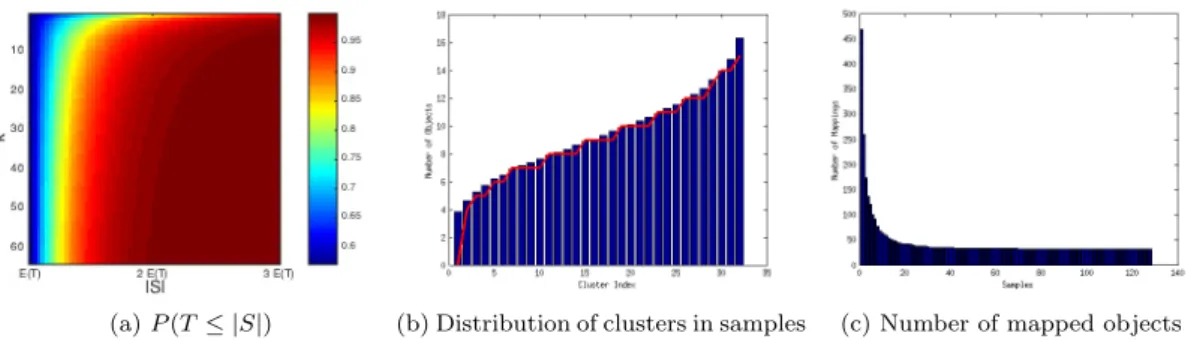
P(Suf f icient(S))≡P(T ≤ |S|)≈e−k·e−|S|/k. (3) Although this may seem problematic, the probability quickly converges, see fig. 1(a)
Another critical observation that needs to be made about a sufficient sample is the distri-bution of the number of objects from each cluster. This can be viewed as a classical occupancy problem. LetXibe the random variable that represents the number of objects inSfrom cluster i. It is well known that
P(Xi=z)≈ 1 z! |S| k z e−|S|/k (4)
which follows a Poisson distribution λkke!λ withλ=|S|/k. Thus, the distribution of the number of objects in the sample set after a sample of size|S|has been drawn follows an inverse Poisson distribution withλ=|S|/k. We found in our experiments that the observed distributions agreed well with the theoretical prediction, see fig. 1(b). This property of the sample data allows for quicker convergence to the solution, see fig. 1(c). It is desirable for each cluster to have a sample set in which it is the most weakly represented among themsets. This criterion turns into a meta version of the coupon collector’s problem where we are interested in the number of sample sets that need to be drawn such that each cluster is the most weakly represented in at least one sample set. For this reason, we usem=k(lnk+γ) as a minimum value form.
3The coupon collector’s problem is a special case of the balls in bins (or urns) problem. Balls in urns is a more general problem where balls are placed into urns of equal probability. This is done until each urn has at leastmballs. In the coupon collector’s problemm= 1.
(a)P(T ≤ |S|) (b) Distribution of clusters in samples (c) Number of mapped objects Figure 1: (a) Probability distribution relationship for P(T ≤ |S|) and number of clusters k. (b)Average distribution of objects in a sample set from each of the 32 clusters for dataset S6, with the theoretical inverse Poisson distribution in red. (c) The number of sampled objects remaining in each sample after removing unmapped objects for dataset S6.
While these classical problems in probability theory provide the theoretical motivation for our algorithm, in practice the parameter|S|will increase depending on the distribution of the data set and the number of sample sets that need to be drawn. In our algorithm, we only use the expectation of the sample set size,E(T), as a starting point for|S|and perform an iterative process of test-and-change to determine the actual sample set size.
4
Experiments
4.1
Datasets
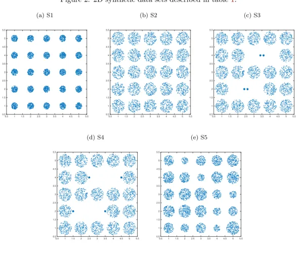
All algorithms were evaluated on 11 published and synthetic datasets of varying size and data distribution (see Table1). The datasets S1-S5 are made up of clusters in two dimensions with a uniform distribution of objects within a circular boundary. S1 and S2 are spaced apart with their cluster centers on a grid, with the only difference being the cluster radii, which are smaller in S1 causing the clusters to be more dense. Dataset S3 has two pairs of clusters that are very near to each other and much more dense. Dataset S4 is a variation of S3 where each of the four dense clusters is near the border of a less dense neighbor. Dataset S5 has cluster centers spaced on a grid with equal density, but the radii are perturbed causing variable size. Dataset S6 is generated by creating well separated Gaussian distributions with variance 1 around the corners of a 5 dimensional hypercube. S7 is a identical to S6, but with more objects. The Yeast dataset4 is a real classification dataset from the UCI Machine Learning repository [8]. D31 [17] is made of 31 randomly placed 2D Gaussian clusters of 100 samples each. R15 [17] is made of 15 similar 2D Gaussian clusters that are positioned in rings. Aggregation [6] contains features that are known to create difficulties for clustering algorithms.
4The Yeast dataset is a benchmark dataset for prediction and clustering algorithms. It is made available by the University of California Irvine. https://archive.ics.uci.edu/ml/datasets/Yeast
Figure 2: 2D synthetic data sets described in table1. (a) S1 0.5 1 1.5 2 2.5 3 3.5 4 4.5 5 5.5 0.5 1 1.5 2 2.5 3 3.5 4 4.5 5 5.5 (b) S2 0.5 1 1.5 2 2.5 3 3.5 4 4.5 5 5.5 0.5 1 1.5 2 2.5 3 3.5 4 4.5 5 5.5 (c) S3 0.5 1 1.5 2 2.5 3 3.5 4 4.5 5 5.5 0.5 1 1.5 2 2.5 3 3.5 4 4.5 5 5.5 (d) S4 0.5 1 1.5 2 2.5 3 3.5 4 4.5 5 5.5 0.5 1 1.5 2 2.5 3 3.5 4 4.5 5 5.5 (e) S5 0.5 1 1.5 2 2.5 3 3.5 4 4.5 5 5.5 0.5 1 1.5 2 2.5 3 3.5 4 4.5 5 5.5
Table 1: Description of synthetic and published data sets.
Dataset (KB) n k dim Description
S1 40 5,000 25 2 Equal size, equal density, well separated S2 40 5,000 25 2 Equal size, equal density, not well separated S3 40 5,000 25 2 Equal size, unequal density, not well separated S4 40 5,000 25 2 Equal size, unequal density, not well separated S5 39.9 4,988 25 2 Unequal size, equal density, not well separated S6 128 6,400 32 5 Unequal size, Gaussian, well separated
S7 1280 64,000 32 5 Unequal size, Gaussian, well separated
Yeast 33.5 1,048 10 8 UCI ML Repository
D31 24.8 3,100 31 2 “A Maximum Variance Cluster Algorithm” [17] R15 4.8 600 15 2 “A Maximum Variance Cluster Algorithm” [17] Aggregation 6.3 788 7 2 “Clustering aggregation” [6]
4.2
Evaluation
To evaluate how AGORAS performs in practice, it was compared it to PAM and CLARANS. All three algorithms were implemented in the C programming language and compiled using gcc version 4.3.4. The synthetic data sets were designed to demonstrate a range of cases that pose problems for partitional clustering algorithms, including clusters that are not well-separated, unequal in size, and unequal in density (see Table1).
For CLARANS, the parameters maxneighbor = 0.0125n and numlocal = 2 were used as recommended by Ng and Han [11]. Both PAM and CLARANS used a random initial config-uration of medoids, with unique pseudorandom seeds for each process. Cluster quality was measured in terms of the standard sum-of-intra-cluster-distance cost value for k-medoids, as well as the pairwiseF1 measure:
F1= 2·precision·recall
precision+recall , Cost(M, D) =
n i=1
dist(Oi, rep(M, Oi)), (5) whereOiis theithobject in the data setD, andrep(M, Oi) is the most similar medoid toOi from the set of medoidsM. The results for CLARANS and AGORAS represent the average of 30 runs, using unique pseudorandom seeds for all of our runs. The time reported for AGORAS includes the time required to partition the data set and determine object membership, though the time taken for loading data into memory is not reported for any of our results. All algorithms used Euclidean distance. The experiments were run on Hopper at NERSC, a Cray XE6, using a single dedicated node. Timing and cluster quality results appear in Table3, while Table 2 gives statistics about the sample size AGORAS for the data sets with equal-sized clusters, along with the probability that every cluster is represented in each sample (P(|S|m)). Note that we did not evaluate PAM on our largest data set (S7) due to its excessively long runtime.
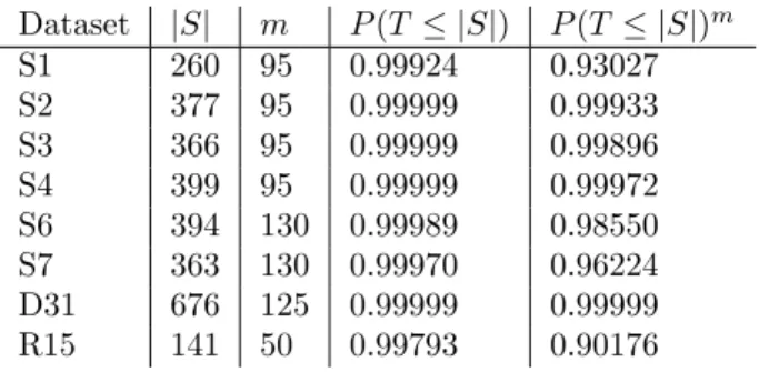
Table 2: Statistics on sample size (|S|) and number of sample sets (m) from AGORAS runs on data sets with equal-sized clusters.
Dataset |S| m P(T ≤ |S|) P(T ≤ |S|)m S1 260 95 0.99924 0.93027 S2 377 95 0.99999 0.99933 S3 366 95 0.99999 0.99896 S4 399 95 0.99999 0.99972 S6 394 130 0.99989 0.98550 S7 363 130 0.99970 0.96224 D31 676 125 0.99999 0.99999 R15 141 50 0.99793 0.90176
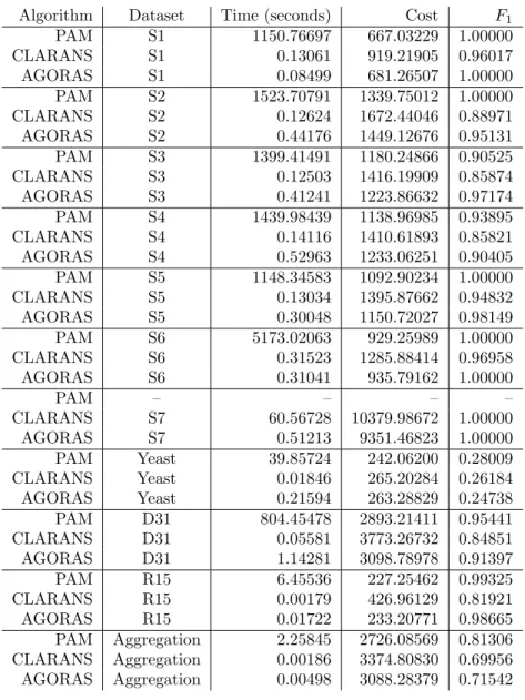
From the results in Table3, PAM took over 1,000 times longer than AGORAS to calculate medoids for S1-S6, which all have 5,000 points, and took over 100 times longer for the smaller, published data sets. While the runtime for AGORAS was greater than the runtime CLARANS on the smaller data sets, AGORAS ran more than 100 times faster than CLARANS on the largest data set (S7), and it is expected that this gap in performance would increase with data size. In addition, AGORAS outperformed CLARANS in terms ofF1measure on all but two of our data sets (S7 and Yeast). As expected, AGORAS clustered the data sets S6 and S7, which come from an identical distribution, in approximately the same amount of time (0.286 sec for S6
vs. 0.263 sec for S7). The difference in time reported in Table3is due solely to the time required to partition the full data set. This observation is confirmation that the runtime of AGORAS is dependent on the distribution of data set and independent of data size, however, AGORAS showed much higher variability in runtime than CLARANS across the 30 runs, possibly due to collisions in mappings from objects on the cluster peripheries or smaller clusters that did not appear in every sample.
Finally, we examined the statistical properties of the samples used by AGORAS in the experiments. We found that the more difficult-to-cluster data sets required a larger sample size on average relative to data set S1 in order to identify thek medoids (see Table2). Also, from Table 2, we can see that the final sample size chosen by AGORAS was large enough to give a 90% chance for all clusters to be represented in every sample. AGORAS performed worst with the yeast data set. Yeast has the most troubling feature for AGORAS—vastly dissimilar cluster sizes. However, we found that it is possible to increase the cluster quality (F1measure) by increasing the number of sample sets,m, beyond our recommended size, which is based on an even data distribution.
5
Conclusion and future work
In this paper we presented a novel sampling-based algorithm called AGORAS for approximating the solution to thek-medoids problem. We showed that AGORAS achieves several orders of magnitude improvement in runtime over existing search based techniques, even for moderate size datasets. We also show AGORAS produces comparable clustering results relative to the well established algorithms fork-medoids. Most significantly, the time required for AGORAS to find clusters in a dataset is dependent on the number of clusters and is effectively independent of dataset size. We see many opportunities for future work. A closer look at Figure 1 suggests an interesting future direction. We may be able to leverage the fact that AGORAS converges very quickly to the appropriate number of clusters in order to develop a parameter-free variation that can automatically detect an appropriate value fork.
Acknowledgement
This work is supported in part by the following grants: NSF awards CCF-1409601, IIS-1343639, and CCF-1029166; DOE awards DESC0007456 and DE-SC0014330; AFOSR award FA9550-12-1-0458; NIST award 70NANB14H012.
Table 3: Timing and cluster quality results for AGORAS, CLARANS, and PAM.
Algorithm Dataset Time (seconds) Cost F1
PAM S1 1150.76697 667.03229 1.00000 CLARANS S1 0.13061 919.21905 0.96017 AGORAS S1 0.08499 681.26507 1.00000 PAM S2 1523.70791 1339.75012 1.00000 CLARANS S2 0.12624 1672.44046 0.88971 AGORAS S2 0.44176 1449.12676 0.95131 PAM S3 1399.41491 1180.24866 0.90525 CLARANS S3 0.12503 1416.19909 0.85874 AGORAS S3 0.41241 1223.86632 0.97174 PAM S4 1439.98439 1138.96985 0.93895 CLARANS S4 0.14116 1410.61893 0.85821 AGORAS S4 0.52963 1233.06251 0.90405 PAM S5 1148.34583 1092.90234 1.00000 CLARANS S5 0.13034 1395.87662 0.94832 AGORAS S5 0.30048 1150.72027 0.98149 PAM S6 5173.02063 929.25989 1.00000 CLARANS S6 0.31523 1285.88414 0.96958 AGORAS S6 0.31041 935.79162 1.00000 PAM – – – – CLARANS S7 60.56728 10379.98672 1.00000 AGORAS S7 0.51213 9351.46823 1.00000 PAM Yeast 39.85724 242.06200 0.28009 CLARANS Yeast 0.01846 265.20284 0.26184 AGORAS Yeast 0.21594 263.28829 0.24738 PAM D31 804.45478 2893.21411 0.95441 CLARANS D31 0.05581 3773.26732 0.84851 AGORAS D31 1.14281 3098.78978 0.91397 PAM R15 6.45536 227.25462 0.99325 CLARANS R15 0.00179 426.96129 0.81921 AGORAS R15 0.01722 233.20771 0.98665 PAM Aggregation 2.25845 2726.08569 0.81306 CLARANS Aggregation 0.00186 3374.80830 0.69956 AGORAS Aggregation 0.00498 3088.28379 0.71542
References
[1] Daniel Aloise, Amit Deshpande, Pierre Hansen, and Preyas Popat. Np-hardness of euclidean
sum-of-squares clustering. Machine Learning, 75:245–248, 2009. 10.1007/s10994-009-5103-0.
[2] David Arthur and Sergei Vassilvitskii. k-means++: the advantages of careful seeding. In
Proceed-ings of the eighteenth annual ACM-SIAM symposium on Discrete algorithms, SODA ’07, pages 1027–1035, Philadelphia, PA, USA, 2007. Society for Industrial and Applied Mathematics. [3] Brian Dawkins. Siobhan’s problem: The coupon collector revisited. 45(1):76, February 1991.
[5] Brian S. Everitt, Sabine Landau, Morven Leese, and Daniel Stahl. Optimization Clustering Tech-niques, pages 111–142. John Wiley and Sons, Ltd, 2011.
[6] Aristides Gionis, Heikki Mannila, and Panayiotis Tsaparas. Clustering aggregation. ACM Trans.
Knowl. Discov. Data, 1(1), March 2007.
[7] Leonard Kaufman and Peter J. Rousseeuw. Finding Groups in Data: An Introduction to Cluster
Analysis (Wiley Series in Probability and Statistics). Wiley-Interscience, March 2005. [8] M. Lichman. UCI machine learning repository, 2013.
[9] J. B. MacQueen. Some methods for classification and analysis of multivariate observations. In
L. M. Le Cam and J. Neyman, editors, Proc. of the fifth Berkeley Symposium on Mathematical
Statistics and Probability, volume 1, pages 281–297. University of California Press, 1967.
[10] Ujjwal Maulik and Sanghamitra Bandyopadhyay. Performance evaluation of some clustering
algo-rithms and validity indices.IEEE Trans. Pattern Anal. Mach. Intell., 24(12):1650–1654, December
2002.
[11] Raymond T. Ng and Jiawei Han. Clarans: A method for clustering objects for spatial data mining.
IEEE Transactions on Knowledge and Data Engineering, 14(5):1003–1016, 2002.
[12] Hae-Sang Park and Chi-Hyuck Jun. A simple and fast algorithm for k-medoids clustering. Expert
Systems with Applications, 36(2):3336–3341, 2009.
[13] David Martin Powers. Evaluation: from precision, recall and f-measure to roc, informedness, markedness and correlation. 2011.
[14] Yaser Sheikh, Erum A. Khan, and Takeo Kanade. Mode-seeking by medoidshifts. InICCV’07,
pages 1–8, 2007.
[15] Weiguo Sheng and Xiaohui Liu. A genetic k-medoids clustering algorithm. Journal of Heuristics,
12(6):447–466.
[16] Catherine A Sugar and Gareth M James. Finding the number of clusters in a dataset. Journal of
the American Statistical Association, 98(463):750–763, 2003.
[17] C. J. Veenman, M.J.T. Reinders, and E. Backer. A maximum variance cluster algorithm. IEEE