MESHFREE METHODS USING LOCALIZED KERNEL BASES
A Dissertation by
STEPHEN TABER ROWE
Submitted to the Office of Graduate and Professional Studies of Texas A&M University
in partial fulfillment of the requirements for the degree of DOCTOR OF PHILOSOPHY
Chair of Committee, Francis Narcowich Co-Chair of Committee, Joseph Ward
Committee Members, Thomas Schlumprecht Fred Dahm
Head of Department, Emil Straube
May 2015
Major Subject: Mathematics
ABSTRACT
Radial basis functions have been used to construct meshfree numerical methods for interpolation and for solving partial differential equations. Recently, a localized basis of radial basis functions has been developed on the sphere. In this dissertation, we investigate applying localized kernel bases for interpolation, approximation, and for novel discretization methods for numerically solving partial differential equations and integral equations. We investigate methods for partial differential equations on spheres using newly explored bases constructed from radial basis functions and associated quadrature methods. We explore applications of radial basis functions to anisotropic nonlocal diffusion problems and we develop theoretical frameworks for these methods.
DEDICATION
ACKNOWLEDGEMENTS
I would like to thank my advisers, Dr. Francis Narcowich and Dr. Joseph Ward, for their continuous support over the years. The countless hours they’ve spent help-ing me with problems, ranghelp-ing from bureaucratic to technical matters, has been invaluable. Always willing to help and always supportive of any new project or in-terest I had, they have made the graduate school experience an enormously fruitful intellectual experience. Their continuous support, which has ranged from giving me gratuitous intellectual freedom to study numerical methods and programming languages on my own, as well as their encouragement to apply for fellowships and writing letters of recommendation is greatly appreciated.
I would like to thank Dr. Rich Lehoucq at Sandia National Laboratories for hosting me as an intern for two summers and for introducing me to interesting new projects that has driven my research at Texas A&M and for supporting my explo-ration of different computer methods and math methods while at Sandia. He encour-aged my initial attempt at a research project and pointed out technical details that helped drive the eventual development of an entire chapter of my thesis. He spent many hours of his time helping me learn to more effectively write and communicate my ideas, which has been a surprisingly non-trivial part of the research experience for me.
I would like to thank Sandia National Laboratories for generously providing me with the Sandia National Laboratories Campus Executive Fellowship, which has had a fundamentally transformative effect on my research and career plans. I would also like to thank the numerous people in the College of Science and Department of Mathematics at Texas A&M University and at Sandia National Laboratories that
provided me help and support as part of the fellowship.
I would be remiss in my acknowledgments if I omitted my friends that have been invaluable over the years. Justin Owen has been a great friend and always there for me throughout the grad school experience. My friend and office-mate Sam Scholze has always made working at school an entertaining experience. He also introduced me to my hobby of weight lifting, which has evolved into the best stress relief hobby I’ve had at graduate school.
Dr. Larson in the Department of Mathematics at Texas A&M introduced me to research for the first time when I was a participant in his Matrix Analysis and Wavelets Research Experience for Undergraduates. Without him, I would certainly not be where I am today mathematically.
I would like to thank the Department of Mathematics at Texas A&M University for the generous support over the years.
TABLE OF CONTENTS Page ABSTRACT . . . ii DEDICATION . . . iii ACKNOWLEDGEMENTS . . . iv TABLE OF CONTENTS . . . vi
LIST OF FIGURES . . . viii
LIST OF TABLES . . . x
1. INTRODUCTION AND BACKGROUND . . . 1
1.1 Radial Basis Functions . . . 2
1.2 Native Spaces . . . 6
1.3 Error Estimates . . . 9
1.4 Spherical Basis Functions . . . 16
1.4.1 Conditionally Positive Definite Kernels on Spheres . . . 20
2. LAGRANGE FUNCTIONS . . . 23
2.1 Lagrange Functions on Spheres . . . 23
2.2 Local Lagrange Functions . . . 33
2.3 Pointwise Convergence of Interpolants and Quasi-interpolants . . . . 40
3. LAGRANGE FUNCTION QUADRATURE . . . 44
3.1 The Quadrature Routine on Spheres . . . 45
4. NONLOCAL DIFFUSION . . . 52
4.1 Nonlocal Vector Calculus . . . 53
4.2 Discretization of the Variational Problem . . . 56
4.2.1 Classical Differential Operators as Limits of Nonlocal Operators 58 4.3 Lagrange Functions and Local Lagrange Functions . . . 58
4.4 Local Lagrange Quadrature . . . 62
4.5.1 Local Lagrange Discretization . . . 65
4.6 Numerical Results . . . 70
4.6.1 Linear Anisotropy Experiment . . . 72
4.6.2 Exponential Anisotropy Experiment . . . 74
4.6.3 Quadrature Experiment . . . 79
4.7 Error Analysis . . . 81
4.7.1 Two Quadrature Error Estimates . . . 81
4.7.2 Local Lagrange Quadrature Error Estimates . . . 87
4.7.3 The Quadrature Error for Solutions to Nonlocal Diffusion Prob-lems . . . 89
4.7.4 An Alternative Nonlocal Diffusion Method . . . 91
5. ELLIPTIC PARTIAL DIFFERENTIAL EQUATIONS ON SPHERES . . 96
5.1 Error Estimates with Spherical Basis Functions . . . 100
5.2 Stiffness Matrix in the Lagrange Basis . . . 105
5.3 Quadrature . . . 111
5.3.1 Numerical Experiments . . . 121
6. RESTRICTED LAGRANGE FUNCTIONS . . . 126
7. SUMMARY AND CONCLUSIONS . . . 159
LIST OF FIGURES
FIGURE Page
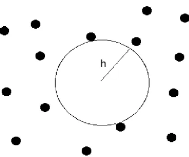
1.1 The dots represent locations of centers. The quantityhrepresents the radius of the largest ball that does not intersect any centers. This quantity measures how dense the data is in the region of interest. . . 12 2.1 A Lagrange function constructed from 625 centers has been evaluated
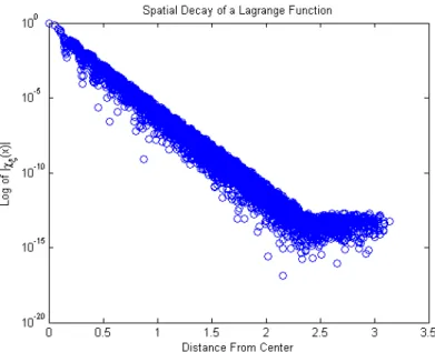
at 5041 points. The distance from the center of the Lagrange function to the evaluation point versus the log of the absolute value of the evaluation of the Lagrange function at the point is plotted. A clear, exponential decay is visible. . . 27 2.2 A Lagrange function centered at a pointξconstructed from 625 centers
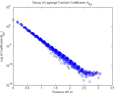
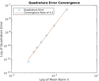
has its coefficients Aξ,η displayed. A clear, exponential decay with respect to the distance d(ξ, η) is visible. . . 31 3.1 The function f(θ) = cos(θ) exp(cos(θ)) is integrated on the sphere
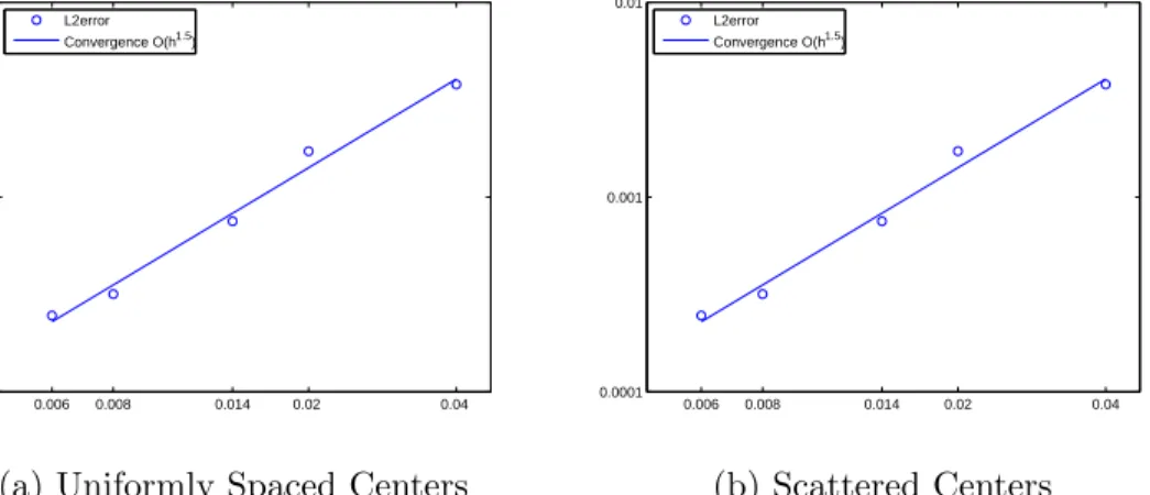
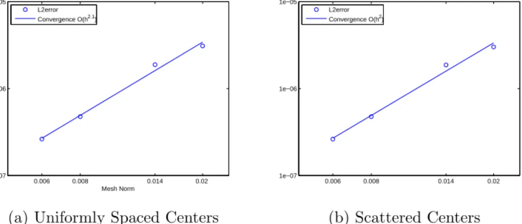
numerically with icosahedral nodes ranging from 2562 nodes to 163842 nodes. The quadrature error decays at a rate of O(h4). . . . 51 4.1 The log of h versus the log of the L2 error for the linear anisotropic
experiment with functions given by (4.19) is displayed. . . 73 4.2 The log ofhversus the log of theL2error for the exponential anisotropy
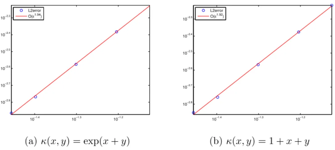
experiment with functions given by (4.20) is displayed. . . 75 4.3 The log of vs. the log of the L2 error of the discrete solutionu,h is
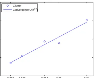
plotted. As goes to zero, we observe 2 convergence. . . . 80 4.4 The log of the quadrature error (4.23) versus the log of the mesh norm
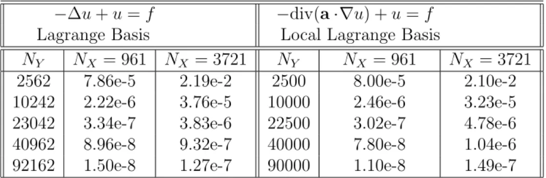
5.1 In (a) and (b), semi-log plots of the errors (adjusted by removing log factors) for −∆u+u=f and −div(a· ∇u) +u =f are shown. The minimum energy points were used for X and icosahedral points were used for Y. In (c), a loglog plot of the L2 error vs. h
X is plotted. For this experiment, the number of quadrature points is fixed and the number of centers used for the approximation space varies. In (d), the log of the condition number for the stiffness matrix for −∆u+u=f is plotted [25]. . . 125
LIST OF TABLES
TABLE Page
4.1 The mesh norm h, number of rows n of the stiffness matrix, and the estimated condition number for the stiffness matrix with the linear anisotropy (4.19) and the exponential anisotropy (4.20). The condi-tion numbers of the stiffness matrices does not increase ash decreases. 75 5.1 Both −∆u +u = f and −div(a· ∇u) + u = f were numerically
solved using minimum energy point sets for X and icosahedral point sets for Y. The L2 error for all cases was O(|log(h
Y)|2h5+Y ). Here, hY =N
−1/2
Y . For the first equation, a Lagrange basis was used, and, for the second, a local Lagrange basis [25]. . . 124
1. INTRODUCTION AND BACKGROUND
A judicious choice of basis can make all the difference in the success of a numerical method. We explore and develop numerical methods for applied problems using a recently developed localized basis of kernel functions. The basis is constructed by linear combinations of radial basis functions. In many ways, this new basis maintains the flexible approximation powers of radial basis functions (RBFs) for scattered data while simultaneously avoiding the downsides of RBF methods. The localized basis enables interpolation of scattered data on manifolds such as spheres and we explore developing an analogous basis in Rd. Due to the desirable properties of the basis for interpolation and approximation, we may consider constructing discretization spaces for solving partial differential equations and integral equations in a variety of settings.
We consider the following classical interpolation problem: let Ω ⊂ Rd be a bounded set and let {xi}Ni=1 = X ⊂ Ω be a set of scattered points (called centers). Let {yj}N
j=1 be a set of known data values e.g., samples of a function yj = f(xj)
. The interpolation problem seeks aninterpolant s: Ω→Rwhich satisfiess(xj) = yj. Let πN(Rd) denote the space of polynomials of degree at most N on Rd. In the case d = 1 with X ⊂ R, the interpolation problem always has a unique in-terpolant s ∈ πN−1(R). That is, there exists a subspace of functions which always
admits a unique interpolant, regardless of the location of the centers. For d > 1, the Mairhuber-Curtis theorem demonstrates that it is not possible to fix a subspace of functions that always admits a unique interpolant regardless of the location of the data sites [28]. This result implies that the interpolants must be constructed by taking into account the configuration of the centers. This raises the difficult problem
of requiring a customized subspace of functions for each different set of centers. 1.1 Radial Basis Functions
One possible solution to the interpolation problem is to useradial basis functions. In this section, we define radial basis functions and we discuss their applications to scattered data interpolation, previous work, and other applications of radial basis functions. Let ϕ(r) : R+ →
R be a continuous function and define the function
Φ :Rd→
Rby Φ(x) =ϕ(kxk). We say such a function Φ isradial. Let Ω ⊂Rdbe a
region of interest where we have some given data. Let {xi}Ni=1 = X ⊂ Ω be a finite set of centers, and define the space
VX = span{Φ(x−xi) :xi ∈X}.
Given data values{yj}Nj=1, we seek an interpolant inVX which is a linear combination of translates of Φ. This leads to a system of N equations in N unknowns with conditions yj = N X i=1 ciϕ(kxj−xik) for j = 1, . . . , N.
If we let Aij =ϕ(kxi−xjk) and let (~c)i =ci and (~y)j =yj, then we seek a solution to the problem A~c=~y. We refer to the matrix A as the interpolation matrix. This leads to the following question: what functions ϕ:R+ →R necessarily generate an invertible interpolation matrix for any set of centers? This problem remains open, but the following restricted question is a classical question in analysis: what functions ϕ generate a positive definite interpolation matrix for all sets of centers? Bochner’s theorem characterizes all positive semi-definite functions as the Fourier transform of a non-negative Borel measure. A useful corollary is that a continuous, integrable function Φ : Rd →
transform is non-negative and non-vanishing. One such example is the Gaussian ϕ(r) = exp(−αr2) forα >0 [28].
A more general notion is that of aconditionally positive definite function of order m. Recall thatπm(Rd) is the space of at most degree m polynomials onRd. We say that ϕ:R+ →
Ris conditionally positive definite of order m onRdif and only if for
any set of scattered centers, the quadratic form N X i=1 N X j=1 αiα¯jϕ(kxi−xjk)
is positive for any set of scalars {αi}N
i=1 not identically equal to zero that satisfy N
X
i=1
αip(xi) = 0
for all p ∈ πm−1(Rd). That is, the interpolation matrix is positive definite on a
subspace “orthogonal” to the polynomials. One such example is the thin plate spline ϕ(r) = r2log(r), which is conditionally positive definite of order 2 on every Rd. Interpolating data on a set of centers with a conditionally positive definite function requires the addition of polynomial constraints to ensure the existence and uniqueness of an interpolant. Given centers {xj}Nj=1 and data values{yj}Nj=1, the interpolation problem is to find coefficients {cj}Nj=1 and {bl}ml=0d such that
yj = N X i=1 ciϕ(kxj −xik) + md X l=0 blpl(xj) subject to N X i=1 cipl(xi) for 0≤l≤md
Radial basis functions have been actively explored for the past several decades. Hardy’s work with the multiquadric was one of the first explorations of radial basis functions for interpolation, dating back to work in 1971. Duchon’s investigation of the thin plate spline used a variational approach of minimizing a semi-norm [5]. The thin plate spline was found to be the minimizer of a certain energy functional (which has a physical interpretation as the bending energy of a thin metal plate). Later, Meinguet pushed forward the use of thin plate spline interpolation for numerical methods [20, 21, 22].
Radial basis functions are actively being researched for discretization methods for partial differential equations. They are particularly intriguing because they do not require a mesh or triangulation and can be used for high dimensional problems. In 1990, Kansa introduced a radial basis function method for the solution of partial differential equations [16]. This work, based on the multiquadric RBF, established the first collocation method for elliptic, parabolic, and hyperbolic partial differen-tial equations. Future work has explored the application of the Kansa method for shocks and shallow water wave equations. Engineers have reported success in using these methods for modeling high order differential equations which often are diffi-cult for finite element methods. Unfortunately, Kansa’s method does not guarantee a solution. Hon and Schaback reported an example of a differential operator, ra-dial basis function, and set of centers which yielded a singular collocation matrix [15]. Furthermore, no error estimates have been proven for Kansa’s method. In con-trast to Kansa’s method, the symmetric radial basis function method introduced by Fasshauer guarantees an invertible collocation matrix and provides error estimates, but at the cost of requiring basis functions to be twice as smooth as Kansa’s method [6].
frame-work for constructing error estimates. Much frame-work over the past several decades has yielded a wealth of theory which can be readily applied to produce error estimates provided the basis of functions being used has known interpolation error estimates. Since radial basis function methods have known error estimates for certain kernels, this suggests a Galerkin method using radial basis functions is viable theoretically. While these have been investigated, due to difficulty with numerically integrating radial basis functions to construct elements in the stiffness matrix, these methods have not been pursued as actively as collocation methods. In contrast to Kansa’s collocation method, Wendland developed error estimates for a Galerkin radial basis function method for elliptic partial differential equations [27].
Radial basis function (RBF) interpolation offers interpolation of possibly highly scattered, high dimensional data. Two computational drawbacks associated with RBF interpolation are the construction of the interpolant and subsequent evaluation of the interpolant. Given N centers, constructing the interpolant requires inverting a matrix where the number of rows is O(N). For globally supported RBFs (e.g., the thin plate splines or Gaussians), the interpolation matrix is dense. The condition number of the interpolation matrix grows with respect to the minimum distance between two centers. Therefore, solving for the interpolant on a large set of centers requires inverting a large, dense, ill-conditioned matrix. The computational cost of evaluating the interpolant on M points is of order O(M N). Fast multipole methods have been investigated to reduce the computational complexity of RBF evaluation, although these methods reduce the accuracy of the interpolant [28].
Radial basis function interpolation has suffered from a so-called trade off prin-ciple. Consider, for example, the positive definite radial basis function ϕ(r) = exp(−αr2) for α > 0. The Gaussian RBF is positive definite on any
Rd, but for
in a well-conditioned interpolation matrix, but yields poor approximation of a func-tion. On the other hand, decreasing α leads to better numerical approximation, but the condition number grows quickly with the number of centers [28]. There is no known analytic method for choosingαand some suggest ad hoc methods of guessing or trial-and-error methods for choosing α. This issue is not unique to the Gaussian; compactly supported Wendland functions also require a user chosen scale parame-ter. The thin plate spline does not require a scale parameter and recent work has demonstrated a “self-scaling” basis which scales automatically with the data density.
1.2 Native Spaces
In this section, we cover background regarding error estimates for radial basis function interpolation on compact domains in Rn. Error estimates for radial basis function interpolation have been a subject of investigation for at least two decades. Most RBF interpolation error estimates take place in the native space, a reproduc-ing kernel Hilbert space correspondreproduc-ing to the (conditionally) positive definite RBF kernel. We discuss these spaces and their importance as well as error estimates for functions not residing in the native space. The error estimates for functions not resid-ing in the native space is crucial for error estimates on partial differential equations and for approximation error from interpolation of lower smoothness functions.
Let H denote a Hilbert space of functions on Ω ⊂ Rn. We say that a kernel Φ : Ω×Ω→R is a reproducing kernel for H if
• 1: Φ(·, x)∈H for all x∈Ω.
• 2: f(x) =hf,Φ(·, x)i for all f ∈H and all x∈Ω.
We say thatH is areproducing kernel Hilbert space and Φ is the reproducing kernel. An example of a reproducing kernel Hilbert space is W21(R) with the reproducing
kernel Φ(·, x) := exp(−1
2|x−·|). Not all Hilbert spaces are reproducing kernel Hilbert spaces. It can be shown that a Hilbert spaceH having a reproducing kernel is equiv-alent to the point evaluation functionals being continuous. A consequence of this result is that L2[a, b] does not have a reproducing kernel since the point evaluation functionals are not continuous.
Positive definite functions naturally relate to reproducing kernel Hilbert spaces. Given a positive definite function, we can directly construct a Hilbert space on which the function is a reproducing kernel. Let Φ : Ω×Ω→ R be a continuous, positive definite function We construct a spaceHΦby considering all finite linear combinations of Φ(·, x). That is,we define
HΦ :={ N
X
j=1
ajΦ(·, xj) :xj ∈X and N <∞} (1.1)
We note that this is a space of continuous functions (since Φ is a continuous positive definite kernel). This space may be equipped with a bilinear form
hf,Φ(·, y)iΦ =f(y)
for all f ∈HΦ and all y∈ Ω. By taking the completion of this space and appropri-ately identifying the elements in the completion as continuous functions, we have a Hilbert space HΦ with a reproducing kernel Φ. The resulting Hilbert space is called the native space of the kernel Φ, under appropriate interpretation of the elements of the Hilbert space as continuous functions. See [28] for a more thorough discussion.
In the context of a conditionally positive definite function, the concept of a native space is significantly more technical. The interested reader is strongly encourage to consult [28] for a much more thorough and full discussion and exposition on the topic
of native spaces and reproducing kernel Hilbert spaces, as well as a complete and rigorous discussion of native spaces for conditionally positive definite functions.
We refer to the Sobolev space on a region Ω, denotedWk
p(Ω) to be the collection of Lp functions with up to order k Lp weak derivatives. That is,
Wpk(Ω) :={f ∈Lp(Ω) :Dαf ∈Lp(Ω) for |α| ≤k}.
The Sobolev space is equipped with the Sobolev norm given by
kfkWk p(Ω) := X |α|≤k kDαfkpLp 1p .
For the casep= 2, which is frequently of interest for our purposes, the Sobolev space is a Hilbert space. In addition to the Sobolev norm on W2k(Ω), we also may use the Sobolev semi-norm given by
|f|Wk 2(Ω) := X |α|=k kDαfk2 L2 12 .
We define the Beppo-Levi spaceBL(Rn) to be the space of functions
BL(Rn) :={f ∈Lp(Rn) :|f|Wk
2(Rn) <∞}.
The Beppo-Levi space is a Hilbert space when equipped with the above semi-norm. We note that polynomials of degree less thankare contained within the kernel of the Beppo-Levi semi-norm.
Rd→R, to be the functions φm(kxk) := kxk2m−d d is odd kxk2m−dlog(kxk) d is even.
These functions are conditionally positive definite of order m. If πm−1(Rd) denotes
the space of degree at most m−1 degree polynomials on Rd, then the bilinear form N
X
i,j
aiajφ(kxi−xjk)>0
provided that PN
i=1aip(xi) = 0 for each p∈πm−1(Rd). Informally, we may interpret
this as the thin plate splines being positive definite on a subspace “orthogonal” to the polynomials of degree at mostm−1. The interpolation space for these functions takes the form
S(X) := {X xi∈X aiφm(· −xi)| X xi∈X aip(xi) = 0 for all p∈πm−1}+πm−1.
Since the φm are conditionally positive definite, on a set of scattered centers X, the interpolation problem has a unique solution provided that the set of centers is unisolvent. We say a set of points X is unisolvent with respect to πm−1(Rd) if the
only polynomial which is zero on all of X is the zero polynomial. We note that this is a mild condition that should not cause issue (except, possibly in the case of very few points or points that lie exactly along a plane or line).
1.3 Error Estimates
We first discuss error estimates for radial basis function interpolation. Histor-ically, these estimates were primarily restricted to functions residing in the native
space of the kernel. This restriction was suspected to be artificial, as numerical experiments with functions not smooth enough to reside in the native space (e.g., Wk
2(Ω)) would still present predictable convergence rates. Characterizing the con-vergence rates requires knowledge of the geometry of the centers. Analogous to the finite element method, where the convergence rate of the scheme depends on the size of the largest elements (denoted by h), radial basis function interpolation conver-gence rates depend on the largest gaps in the distribution of the centers (a quantity aptly also denoted by h). We note that the radial basis function estimates are anal-ogous to the error estimates typically derived for finite element schemes; typically, one expects the solution to a function in Wk
2(Ω) to converge at a rate of O(hk) in the L2 norm. Additionally, one expects the solution to converge at a rate ofO(hk−α) in the Wα
2 (Ω) norm. Such results have been developed for radial basis functions and we present them below.
The geometry of the data affects the quality of the interpolant in multiple ways. Informally, if the data is sufficiently “dense” in the domain, we expect the interpolant to provide a high degree of approximation to a smooth function. Furthermore, the distribution of the points may affect the quality of the interpolation matrix. If two centers xi, xj are very close, then the i and j columns of the interpolation matrix are very “similar”, which causes the condition number of the matrix to be poor. Therefore, the challenge for scattered data interpolation is to have well-distributed data that is sufficiently dense, yet does not clump. We mathematically characterize these ideas with different quantities to represent the geometric properties of the data. Let X ⊂ Ω be a collection of scattered centers. We define the mesh norm or fill distance h to be the radius of the largest ball in Ω that does not intersect X. We define the separation radius q to be half the minimum distance between centers.
Mathematically, h:= sup x∈Ω min xi∈X kx−xik q:= 1 2xi,xinfj∈X kxi−xjk. (1.2)
See Figure 1.1 for a visual example of the mesh norm. We define the mesh ratio ρ := h
q. Informally, forρ near one, the centers are nearly uniformly distributed and large ρ indicates clustering of points. Let {Xh,q} be a collection of sets of centers indexed by mesh norm h, q. We say the collections of centers are quasi-uniformly distributed if there exists constants C1, C2 such that
C1q≤h≤C2q.
Consequently, sup{X
h,q}ρh,q ≤
C2
C1, which implies the mesh ratio is bounded.
Quasi-uniformly distributed collections of centers allow for theoretically shrinkinghto zero while controlling the distributions of the centers so they do not clump arbitrarily as h→0. This is a fundamental assumption we assume throughout.
Now that we may quantify geometric properties of the centers, we present a classical radial basis function theorem for interpolation error estimates.
Theorem 1. [28] Suppose that Ω ⊆ Rd is bounded and satisfies an interior cone condition. Let Φ(x) = (−1)k+1kxk2klog(kxk) and let f ∈ N
Φ(Ω). Let X be a collection of quasi-uniformly distributed centers and let IXf denote the radial basis function interpolant constructed using Φ. Then, there exists C > 0 such that for sufficiently small h,
|Dαf(x)−DαIXf| ≤Ch k−|α|
Figure 1.1: The dots represent locations of centers. The quantity h represents the radius of the largest ball that does not intersect any centers. This quantity measures how dense the data is in the region of interest.
Analogous results hold for compactly supported Wendland functions. The key observation in the above theorem is that the functionf lies in the native space. This assumption is highly restrictive, so error estimates for functions not contained in the native space are of interest. The restriction of error estimates for functions only residing in the native space was a limiting factor for the theoretical development of error estimates for methods in partial differential equations. Work by Narcowich, Ward, and Wendland proved that error estimates can “escape” the native space for certain radial basis functions [26]. We present an example of such an “escape” estimate which will prove to be useful for our purposes later.
an interior cone condition. For sufficiently small h, and f ∈Wk
2(Ω) for d2 < k≤m,
kf −IXfkL2(Ω) ≤ChkkfkWk
2(Ω)
where IXf ∈W2m(Ω) is the thin plate spline interpolant [26].
We briefly remark that the restriction k > d2 is imperative. If k ≤ d
2, then f is not necessarily a continuous function; by the Sobolev embedding theorem, Wk
2(Ω) are continuous for k > d2. Hence interpolation is a questionable operation.
The proof of this theorem relies on a very important lemma that is interesting in its own right. The so-called “Zeros lemma” relates different Sobolev norms of a function that has sufficiently many zeros within a region.
Proposition 1. Let Ω ⊂ Rn be a bounded and satisfy an interior cone condition. Let k be a positive integer with 0 < s ≤ 1, 1 ≤ p, q ≤ ∞ and let m ∈ N satisfy k > m+dp for p >1 or k ≥m+d for p= 1. Let X be a set with mesh norm h that is sufficiently small. If u∈Wk+s p (Ω) satisfies u|X = 0, then |u|Wm q (Ω) ≤Ch k+s−m−d(1 p− 1 q)+|u| Wpk+s(Ω).
In particular, for the choice q = p = 2 and s = 0 (i.e., a non-fractional or-der Sobolev space), we have |u|Wm
2 (Ω) ≤ Ch
k−m|u| Wk
2(Ω). As one might suspect, by
noting that a function u and its radial basis function interpolant are zero on the set of centers, an error estimate for |u−IXu|Wm
2 (Ω) can be derived. Since the thin
plate splines have error estimates which escape the native space and require no scale parameter, they are of particular interest for numerical methods besides interpola-tion. We use these approximation powers later for work involving partial differential equations and nonlocal diffusion. We briefly remark on the approximation powers of
alternative radial basis functions. The Gaussians and multiquadrics enjoy a spectral convergence result for functions in their native space [18]. That is, for f ∈ NΦ(Ω), the native space for the Gaussian kernel,
kf−IXfkL∞(Ω) ≤Cexp − c h kfkNΦ(Ω).
For functions in the native space, the interpolant rapidly converges to the function at an exponential rate. However, the trade off is the small size of the native space. Elements of the native space for Gaussians and multiquadrics are necessarily analytic, which is a “small” space. In contrast, the thin plate splines guarantee convergence to less smooth functions. In particular, it has been shown that error estimates for functions outside of the native space exist.
Now that we have some understanding of the approximation powers of radial basis functions, we consider how numerically stable the construction of the interpolant is. The construction of the interpolant requires the solution of a linear system of equations, and hence the solution of a matrix equation via some iterative method or by LU decomposition. The solution of a matrix equation by iterative methods can be sensitive to noise in the data, which is a guaranteed reality since computers are involved. The condition number of a matrix measures, roughly, how much small perturbations in the data affect the solution to a problem. For a matrix A, we define the condition numberκ(A) :=kAk kA−1k. In the lucky case of a symmetric, positive definite matrix, we know kAk = sup{λ : λ ∈ σ(A)} where σ(A) is the collection of eigenvalues of A. Furthermore, kA−1k is the reciprocal of the minimal eigenvalue of A. Therefore, we have κ(A) := λmin(A)
λmax(A).
Constructing an accurate solution to a linear system of equations is problem-atic for “very large” condition numbers. Understanding how the condition number
changes as parameters for a problem are modified is imperative. For the problem of radial basis function interpolation, the condition number can be characterized in terms of the separation radius q. (We note that, in the quasi-uniform assumption, this number can be bounded above and below by the mesh norm h). The depen-dence on q is perhaps not particularly surprising; asq shrinks, the centers get closer and closer. Consequently, two columns of the interpolation matrix will be very close componentwise, which implies the matrix becomes “more and more nearly linearly dependent”.
We can quickly measure an upper bound on the maximal eigenvalue for kernels. To approach this problem, the Gershgorin Circle Theorem for eigenvalues provides a method to approximate upper bounds on the difference between matrix entries and eigenvalues:
|λ−aii| ≤
X
i6=j ai,j
where ai,j are the (i, j) matrix entries. For an interpolation matrix, ai,j = Φ(xi, xj), and consequently, |λmax(A)−Φ(xi, xi)| ≤X i6=j |Φ(xi, xj)| ≤(N −1)kΦ(·,·)kL∞ Consequently, |λmax| ≤NkΦ(·,·)kL∞ ≤Cq−dkΦ(·,·)kL∞.
The last inequality follows by a simple bound on the number of centers in a region Ω ⊂ Rd. A significantly more difficult problem is analyzing lower bounds for the minimal eigenvalue. We refer the interested reader to [28] for a thorough discussion, but we present some results here. For the thin plate splinesφ(r) = (−1)k+1r2klog(r), the minimal eigenvalue falls asq2k. Consequently, asqgoes to zero, the interpolation
system may become ill-conditioned. For this reason, constructing an interpolant on a large set of centers with a small separation radius may be difficult. Solving, large, dense, ill-conditioned linear systems is a non-trivial computational challenge. Furthermore, poor condition numbers degrade the performance of iterative methods. This issue is one of many which motivates our future work with an alternative basis. We remark briefly on alternative radial basis functions. The compactly supported Wendland functions also possess an algebraic rate of change in the minimal eigen-value. On the other hand, the Gaussians suffer from an exponential decrease in the minimal eigenvalue, which leads to unpleasantly ill-conditioned systems even for small collections of centers.
1.4 Spherical Basis Functions
The problem of interpolation on Riemannian manifolds is of interest for scientific applications. In particular, much work has been done in the case of a boundaryless, compact Riemannian manifold, such as the n-sphereSn. In the case of
Sn,spherical
basis function (SBF) interpolation has been explored and allows for interpolation of scattered data. Excluding a few special cases for point distributions along pla-tonic solids, constructing uniformly spaced points along the sphere is not possible. Methods requiring regular distributions of points are not available. Therefore, inter-polation methods which allow for scattered data are imperative for spheres.
Given a set of points (centers) distributed along the n-sphere, a spherical basis function Φ : Sn ×
Sn → R can be defined by choosing Φ(x, y) = φ(x·y) for φ :
[−1,1] → R. For each center xj ∈ {xi}Ni=1, the spherical basis function is the rotation to the point xj, Φj(x) = φ(x·xj). The interpolant is then formed from
linear combinations of rotations of Φ, given by s(x) = N X j=1 cjφ(x·xj).
Positive definite spherical basis functions, analogous to positive definite radial basis functions, yield positive definite interpolation matrices. Conditionally positive defi-nite kernels, such as the restriction of the thin plate spline toSn, may also be defined in a similar fashion. While these methods offer interpolation for highly scattered data, they suffer the same drawbacks as the radial basis functions on domains in
Rn. In particular, we are interested in the restricted surface splines or polyharmonic
splines
φm(x·y) := (−1)m(1−x·y)m−1log(1−x·y)
for m≥ n 2.
We discuss in detail later partial differential equations on spheres, which neces-sitates some discussion of background. We focus on the n-sphere with an interest in differential operators, spherical harmonics, Sobolev spaces, and approximation spaces on spheres. The sphere Sn is a compact, boundaryless Riemannian manifold. Let (x1, x2, . . . , xn) be a smooth set of local coordinates. The sphereSn has a metric tensorgij and measuredµ=
p
det(gi,j)dx1dx2. . . dxn. We are particularly interested in the case n = 2, which is the usual sphere. In this case, we have the usual local spherical coordinates (θ, ϕ), where θ is the colatitude and ϕ is the longitude. With
these local coordinates, the metric tensor takes the form gij = 1 0 0 sin2(θ) .
Differential operators on spheres are of particular interest since we aim to dis-cretize and solve partial differential equations on the sphere. The covariant derivative operator,∇, acts as the usual gradient when operating on functions expressed appro-priately. The Laplace-Beltrami operator acts as a spherical analogue of the Lapla-cian. The Laplace-Beltrami operator is defined as ∇∗∇, which in local coordinates may be expressed as ∆u:= p 1 det(gij) X i,j ∂ ∂xi q det(gij)gij ∂u ∂xi (1.3)
where gij is the inverse matrix of g
ij. As usual, we are particularly interested in the case of S2, which in spherical coordinates leads to the Laplace-Beltrami operator taking the form
∆u= 1 sin(θ) ∂ ∂θ sin(θ)∂u ∂θ + 1 sin2(θ) ∂2u ∂φ2. (1.4)
The eigenfunctions of the Laplace-Beltrami play an important role on the sphere and we make use of them as a basis in our numerical methods. These eigenfunctions, known as the spherical harmonics, are eigenfunctions of −∆ on Sn with eigenvalues λ` = `(`+n −1). The eigenspace corresponding to λ` is spanned by a collection of orthonormal eigenfunctions denoted by Y`,k where k = 1, . . . , d`. We denote the eigenspace spanned by {Y`,k}d`
k=1 = H`. The space spanned by all eigenfunctions up to order L will be denoted by ΠL := ⊕L`=0H`. The dimension of the eigenspace
H` ∼O(`n−1). Letx, y ∈Sn and let x·y denote the dot product inRn+1. Then, the
famous addition formula tells us d` X k=1 Y`,k(x)Y`,k(y) = 2`+n−1 (n−1)ωn P n−1 2 ` (x·y)
whereωnis the volume ofSnandP
n−1 2
` is the degree of the`ultraspherical polynomial of order n−12 . For the casen = 2, these polynomials are the Legendre polynomials.
The spaceL2(
Sn) is the Hilbert space of square integrable functions with respect
to the measuredµ. An orthonormal decomposition ofL2 functions is provided by the spherical harmonics. As a complete orthonormal set, we may expand anyf ∈L2(
Sn)
via the formula
f = ∞ X `=0 d` X k=1 ˆ f`,kY`,k.
It then follows that the L2 inner product of f, g∈L2(Sn) is given by
hf, giL2( Sn) = ∞ X `=0 d` X k=1 ˆ f`,kgˆ`,k.
In addition to L2(Sn), we require Sobolev spaces on spheres so we may char-acterize the smoothness of the functions we are working with. This is invaluable for partial differential equations, as error estimates often depend on some notion of smoothness. Furthermore, regularity theorems guarantee smoothness properties of the solution provided some level of smoothness on the data. We define the Sobolev space of order m to be the collection of functions
Hm :={f ∈L2(Sn) : ∞ X `=0 d` X k=1 (1 +λ`)kfˆ`,k2 <∞} (1.5)
which has an inner product given by hf, giHk(Sn) := ∞ X `=0 d` X k=1 (1 +λ`)kfˆk,`gˆk,`.
We note that we may also denote Hm by W2m(Sn) to match our notation for Rn. Fractional order Sobolev spaces extend the definition above. For fractional τ, we may define Hτ as the space of functions such that k(I−∆)
τ
2fkL2(Sn)<∞.
We note that the Laplace-Beltrami operator is a self-adjoint operator with respect to the L2(
Sn) inner product and −∆ is positive on the orthogonal complement of a
finite dimensional subspace of spherical harmonics.
1.4.1 Conditionally Positive Definite Kernels on Spheres
A kernel κ is conditionally positive definite with respect to a finite dimensional subspace Π if, for any set of N distinct centers, the matrix KX :=
κ(ξ, η)
ξ,η is positive definite on the subspace of all vectors a ∈ CN satisfying P
ξ∈Xaξp(ξ) = 0 for all p∈Π.
In the case of the sphere S2, we focus on the finite dimensional subspaces ΠL of degree at most L spherical harmonic polynomials. By a slight re-indexing of the {Yl,k}, we may write them as a collection of orthonormal functions {φj}. We now consider a class of conditionally positive definite kernels that we characterize by studying their expansion in terms of the orthonormal basis{φj}. Let{κj}∞j=1 ∈`2(N) with all but finitely many κj positive. Then, we consider the kernel κ of the form
κ(x, y) :=X j∈N
k(j)φj(x) ¯φj(y). (1.6)
Such a kernel is conditionally positive definite with respect to the space Π := span{φj : κj ≤ 0}. LetJ denote the set of indices so that κj ≤ 0. To verify
condi-tionally positive definite, we consider P
ξ,ηαξκ(ξ, η) ¯αη for some arbitrary collection of centers X with ξ, η ∈ X and some arbitrary collection of coefficients {αξ}ξ∈Ξ such that P
j∈Jαξφj(ξ) = 0. Then, we compute by expanding κ in terms of the orthonormal basis X ξ,η αξκ(ξ, η) ¯αη =X j∈N κjX ξ,η αξφj(ξ)φj(η)αη =X j /∈J κjkαξφj(ξ)k`2(X) >0.
As we know, conditionally positive definite kernels give rise to unique interpolants provided additional constraints from some finite dimensional subspace Π are in-cluded. Using a kernel of the form Equation (1.6), an interpolant to a function f is constructed by IXf(·) = X ξ∈X aξκ(·, ξ) +X j∈J bjφj(·) where we know P
ξ∈Xaξφj(ξ) = 0 for allj ∈J. Constructing the interpolant to the function f by data samples {f(ξ)}ξ∈X follows by solving a matrix problem of the form KX P PT 0 a c = f 0 (1.7)
where (KX)ξ,η = κ(ξ, η) and (Φ)ξ,j := φj(ξ). As we know, this matrix system is invertible since κ is a conditionally positive definite kernel with respect to Π. Fur-thermore, the interpolant can be viewed from an alternative, variational perspective. The interpolant is a minimizer of a certain variational problem involving a semi-norm induced by the coefficients.
We define the native space inner product corresponding toκ by hf, giκ = X j∈N ˆ fjφj, X j∈N ˆ gjφj k :=X j /∈J ˆ f(j)ˆg(j) κj (1.8)
where ˆfj denotes the Fourier coefficient of f with respect to the orthonormal basis
{φj}. We note that this is certainly asemi-inner product and not a true inner prod-uct. Consider, for example, applying the above semi-inner product to functions in Π; the semi-inner product yields zero since the sum runs over j /∈J. The semi-inner product induces a semi-norm in the usual way by |f|2
k = hf, fik. The interpolant constructed by solving (1.7) minimizes the semi-norm | · |k.
2. LAGRANGE FUNCTIONS
Radial basis functions present numerous advantages for numerical methods, such as impressive interpolation and approximation powers. Well-understood convergence rates for interpolation as well as characterizations of the stability of interpolation matrices support the notion that, theoretically, radial basis functions may be potent tools for developing numerical methods for problems involving scattered, irregular data. However, difficulties arise in the implementation of the methods. Solving ill-conditioned, dense linear systems can be a non-trivial computational burden. We present methods that enable one to maintain all the benefits of radial basis func-tions while simultaneously reducing the computational overhead. To achieve this, we change from the basis of translates of a kernel Φ(kx−yk) to a basis of functions which interpolate one at a single point and zero elsewhere. These functions we refer to as Lagrange functions (others may refer to these as cardinal functions).
Lagrange functions and local Lagrange functions are the primary objects of inter-est for constructing numerical methods. The choice of basis can impact the efficacy of a numerical method, and we demonstrate that the local Lagrange functions perform admirably. In this chapter, we discuss in detail Lagrange functions and local La-grange functions. We provide background information necessary to understand their theoretical properties and we provide some numerical experiments demonstrating the theoretical properties.
2.1 Lagrange Functions on Spheres
We begin our discussion of Lagrange functions by focusing on Lagrange functions on the n−sphere, Sn. The manifold
Snhas numerous advantageous properties, most
theoretical difficulties which arise during the case of bounded subsets of Rn. In particular, we note that the boundary is a nuisance ubiquitous throughout the field of numerical methods. By working on a manifold without boundary, we avoid many of these issues.
We start by considering a set of quasi-uniformly distributed centersX ⊂Sn. We restrict our focus to the surface splines of order m defined by
φm(x, y) := (1−x·y)m−1log(1−x·y).
We know this is a conditionally positive definite spherical basis function with respect to the space Πm(Sn). The approximation space VX is defined to be the collection of acceptable linear combinations of rotations of φm(x·xj) plus polynomials of up to a certain degree. That is,
VX :={X xj∈X ajφm(x·xj) + Πm : N X j=1 ajp(xj) = 0 ∀p∈Πm}.
We consider changing from this basis of rotations of φ(x·xj) to a basis which is highly localized spatially. Let xj ∈ X and consider constructing the interpolant, denoted χj, that takes a value of one atxj and zero elsewhere. That is, χj(xi) = δi,j where δi,j = 0 if i6=j and 1 if i =j. We know that for any collection of unisolvent centers, there always exists a unique interpolant to any data condition on the centers, so we know χj must exist in VX. To construct this function, we enforce for each
ξ ∈X, χj(ξ) = N X i=1 αi,jΦ(xi, ξ) + m X `=0 d` X k=1 β`,k,jY`,k(ξ), 0 = N X i=1
αi,jp(xi) for all p∈Πm.
Consequently, enforcing this condition requires the solution of a linear system of size O(N). By quasi-uniformity, we know that q ∼ CN1d, and as N grows, the
condition number gets progressively worse with a decrease of the minimal eigenvalue algebraically in terms of q. Consequently, the construction of the Lagrange function requires solving a large, dense, possibly ill-conditioned linear system of equations. Furthermore, to construct the full basis,N such systems must be solved. The reader may be very suspicious of any possible numerical use or practical application of such a basis; this skepticism is warranted, and indeed, we do not suggest the use of this basis for application necessarily. We later present a computationally friendly basis which preserves many of the properties of the Lagrange basis. However, before we discuss this basis, we present background information required which we take advantage of for our purposes later.
We begin our discussion of results on Lagrange functions on spheres by presenting estimates on their norms. To do so, interpolation error estimates for spherical basis functions are used, which are based on the powerful “Zeros Lemma” for Riemannian manifolds. The first observation is that the Lagrange functions, for various quasi-uniform sets, are pointwise bounded above. This prevents the possibility of the Lagrange functions “spiking” up too high or low off of the centers as the mesh norm h gets small. Indeed, the bound depends on the mesh ratio, which is bounded under the quasi-uniform assumption.
Lemma 1. The Lagrange functions are uniformly bounded by constants independent of h or q.
We next note a remarkable property of the Lagrange functions on the sphere: they are highly spatially localized. Indeed, the Lagrange function centered at a point xj exponentially decays with respect to the distance from the center xj. One may erroneously view this as unsurprising; χj certainly is zero on all of the centers except one, so it being small may not seem surprising. However, functions that interpolate zero throughout might still posses wild oscillations between the centers. Apparently, the Lagrange functions for thin plate splines do not. Furthermore, this is surprising because of the structure of a thin plate spline; these functions grow with distance and are categorically not localized spatially in any way. However, the correct linear combinations of thin plate splines plus the appropriate polynomial apparently results in a highly localized function.
Proposition 2. [13][Proposition 4.5] Suppose that m > d2 and κm is a polyharmonic kernel on Sn. There exist positive constants h
0, ν, and C independent of h and q so that for any set of quasiuniform centers X with mesh ratio ρ and sufficiently small mesh norm h, the Lagrange function centered at ξ∈X satisfies
|χξ(x)| ≤Cρm− d 2 exp − ν hd(x, ξ) .
This argument was developed in [13] and also in [10]. The argument is based off of a trick showing that the bulk of the Sobolev semi-norm of the Lagrange function was contained in a thin annulus about the center. This “bulk chasing” argument was inspired by a similar result due to Matveev, which he used for working with Dm splines on Rn [19]. For more general manifolds, the decay results can be extended but with a modification that the decay is not in terms of just d(x, ξ), but in terms
Figure 2.1: A Lagrange function constructed from 625 centers has been evaluated at 5041 points. The distance from the center of the Lagrange function to the evaluation point versus the log of the absolute value of the evaluation of the Lagrange function at the point is plotted. A clear, exponential decay is visible.
of min d(x, ξ), rM where rM denotes the injectivity radius of the manifold. The argument for the decay largely takes place in the tangent space, which converts the problem from a problem on manifolds to a problem in Rn, which is where the injectivity radius factors in.
In addition to the spatial decay of the Lagrange functions, they also exhibit a special H¨older continuity type of estimate.
Proposition 3. [12] Under the assumptions of Proposition 2, for any 0 < ≤ 1, there exists a constant C depending on the mesh ratio, the order m of the basis function κm, and , so that
|χj(x)−χj(y)| ≤C d(x, y) q .
These results suggest the basis behaves well: the basis functions are spatially localized with predictable continuity patterns. These results enable one to begin proving results about the stability of the basis. The first result that we present from [13] is one that studies the Lebesgue constant of the basis.
The Lebesgue constant corresponding to the collectionX of centers is defined to be L(X) := supx∈Sn
P
ξ∈X|χξ(x)|. This quantity measures the stability of the inter-polation process. If this quantity grows without bound as h → 0 for quasi-uniform sets, the interpolation operation becomes increasingly unstable. Consequently, the coefficients for the interpolant can grow without bound, as may happen with the case of using the basis of translates {κ(·, ξ)}. The Lebesgue constant depends fundamen-tally on the choice of basis; alternative bases for the same approximation space may lead to different results. Therefore, establishing a uniformly bounded Lebesgue con-stant independent of mesh norm suggests the Lagrange bases provide stable methods for interpolation even as the mesh norm becomes quite small.
This should be contrasted with the case of other interpolation methods, such as interpolation via spherical harmonic polynomials. This method is indeed unstable [13]. It can be shown that spherical harmonic polynomial interpolation suffers from a Lebesgue constant that grows as Ld−21 where L is the highest degree of spherical
harmonic used. On the real line, equidistant nodes yield an exponentially growing Lebesgue constant, which suggests interpolation can become problematic.
Proposition 4. [13] Under the assumptions of Proposition 2, the Lebesgue constant is bounded by a constant depending only on the kernel, the mesh ratio ρ, and the manifold.
A bounded Lebesgue constant provides a wonderful result which suggests that interpolation with the SBFs we employ is a near best approximation in L∞. In
general, given a finite dimensional subspace of continuous functions, it does not follow that using these functions to interpolate data provides in any way optimal approximation. Polynomial interpolation can wildly oscillate yielding diverging L∞ error. However, as a result of a bounded Lebesgue constant, an interpolation scheme yields near optimal approximation. Let IXf denote the interpolant and VX the approximation space using the centers X and a kernel κm with bounded Lebesgue constant. Then, given any other function g in the approximation space, we know IXg =g, and we can bound
kf −IXfkL∞ =kf −g+g−IXfkL∞ =kf −g+IX(f −g)kL∞
≤ kf −gkL∞ +kIX(f −g)kL∞ = (1 +L)dist(f, VX) = (1 +L) inf
g∈VX
kf −gkL∞.
What this suggests is that interpolation is near optimal in the L∞ norm. This result is analogous to, for example, Cea’s lemma, which states the Galerkin solution to a bilinear problem is near optimal in the Hilbert space norm of choice. This invaluable result is often the first step in an error estimate for a discretization method for partial differential equations.
Combining techniques from the exponential decay of the Lagrange functions as well as the bounded Lebesgue constant properties led to the development of norm inequalities that enable one to bound the so-called “condition numbers” of the La-grange functions. Let {vξ}ξ∈X be a basis for an approximation space. We define the condition numbers to be the values C1,p, C2,p so that
C1,pk{aξ}k`p(X) ≤ k X
ξ∈X
The constants depend in some way upon the basis and upon p. Having condition number bounds of this form suggests the basis is Lp stable. That is, the Lp norm of the interpolant is comparable to the `p norm of the coefficients. Besides being useful for theoretical purposes, understanding theLp condition numbers enables one to make estimates for condition numbers of matrices arising from the discretization of partial differential equations and integral equations.
Proposition 5. [7] Let X be a quasi-uniformly distributed set of centers. There exist constantsc1 andc2 depending only onm, the order of the SBF, andρ, the mesh ratio, so that for sufficiently small mesh norm h, the Lagrange functions satisfy the condition number estimates
c1q d pk{a j}k`p(X) ≤ k X ξ∈X aξχξkLp(Sd) ≤c2q d pkak `p(X).
To be clear, this result is not limited to merely one collection of centers X; this holds as we shrinkh, q →0, provided the sets of centers satisfy the quasi-uniformity assumptions (that is, C1 ≤ hqXX ≤ C2 for some fixed C1 and C2 independent of X). An immediate consequence of this statement is that theLp norm of a single Lagrange function is on the order of qdp.
Proposition 6. [7] Let X be a set of quasi-uniformly scattered centers in Sn and let χξ, χη denote Lagrange functions for the points ξ, η ∈ X. Assume the ap-proximation space is generated by a conditionally positive definite kernel κ(·, ξ) =
P
j∈Nκjϕj(·)ϕj(ξ). The Lagrange function χξ has expansion χξ(·) :=
X
η∈X
Aη,ξκ(·, η) +pξ
Figure 2.2: A Lagrange function centered at a point ξ constructed from 625 centers has its coefficients Aξ,η displayed. A clear, exponential decay with respect to the distance d(ξ, η) is visible.
As a consequence of this, it has been demonstrated that the Lagrange function coefficients decay exponentially. The result follows by a type of Cauchy-Schwarz inequality that was presented in [7].
Proposition 7. [7] Let X be a quasi-uniformly distributed set of centers on the sphereSn with sufficiently small mesh normh. Then, the coefficients of the Lagrange function χξ satisfy |Aη,ξ| ≤Cq1−mexp −νd(ξ, η) h . (2.1)
The significance of Proposition 7 is that the Lagrange functions are not solely localized spatially. The Lagrange functions, in the words of the authors of [7], have
a “small footprint” in the kernel basis. While each Lagrange function is a linear combination of all rotations of the kernel κ(·, η), apparently only kernels centered near ξ contribute significantly to the total value of the Lagrange function. The exponential decay forces the coefficients Aξ,η to be small for d(ξ, η) large enough. This is highly suggestive of the idea that perhaps the Lagrange functions can be constructed in a way that takes advantage of this spatial locality while not reducing the approximation power of the functions.
The last major property we mention is the ability to switch between to relate different order Sobolev norms of linear combinations of basis functions. These are often referred to as Bernstein estimates. Let VX be the space generated by the restricted surface splines (we sometimes refer to them as thin plate splines) ϕs(t) = (−1)s+1(1−t)slog(1−t).
Proposition 8. [24] Let g ∈ VX which is generated by the thin plate spline for a quasi-uniform set of centers X ⊂ Sn. Then, there exists a constant C independent of q, h such that
kgkWk
2(Sn) ≤Cq
−kk
gkL2(Sn).
This result can be extend to handle Lp spaces instead, but our primary focus is on L2.
We close this section by summarizing the key points developed by different au-thors over several years. The Lagrange functions of conditionally positive definite functions on manifolds are highly spatially localized as well as localized in the sense that the coefficients decay rapidly. The basis is inherently stable with a bounded Lebesgue constant as well as computable upper and lower condition number bounds. The Lp norm of a linear combination of Lagrange functions is comparable directly to the `p norm of the sequence of coefficients, with a factor of qdp to be included.
Finally, switching between Sobolev norms induces a penalty of q−k, where k is the difference between the order of the Sobolev spaces.
2.2 Local Lagrange Functions
We discuss results in this section regarding the development of a highly spatially localized, “small-footprint” basis. By small-footprint, we mean each basis element is constructed from few kernels, relative to the total number of kernels. The local basis retains many of the advantages of the full Lagrange basis discussed in Section 2.1. In particular, they decay quickly away from their center, are Lp stable, and provide near optimal approximation.
While the full Lagrange basis enjoys numerous theoretical advantages, the com-putational difficulty of assembling the Lagrange functions impedes their use in appli-cation. Developing a basis of functions which approximates the Lagrange functions has been a topic of some interest. Previous efforts have considered ad hoc methods of constructing Lagrange functions using few centers clustered around a center, but there was no strategy for choosing the number of centers nor for how the number of centers chosen should change as the mesh norm decreased. The results in [13] and [14] suggested that the Lagrange functions were highly localized spatially. Indeed, Proposition 2 suggests the Lagrange function is nearly zero for far away points. That the coefficients also decay exponentially, as shown in Proposition 7, suggested that a function that mimics the properties of the Lagrange function could be constructed that only requires a small number of kernels, rather than being a linear combination of every kernel. In [7], these ideas are explored and a full theory has been developed for a localized collection of Lagrange functions, referred to as local Lagrange func-tions; provable, theoretically supported bounds for the number of centers required for the construction of each local basis function are presented.
We begin by presenting the algorithm for the construction of the local Lagrange functions. We then discuss their theoretical properties. We encourage the interested reader to read [7] for a thorough and detailed account of the theoretical properties. LetX ⊂S2be a collection of quasi-uniformly scattered centers with mesh normhand separation radius q. We focus on the thin plate spline kernel κm(t) = (−1)m−1(1− t)m·log(1−t), which is a conditionally positive definite function with respect to the space Πm of at most degree m spherical harmonics. The (full) Lagrange function at the point ξ ∈ X is χξ(·) = P
ηaξ,ηκ(·, η) +
PL
k=1bk,ξψk(·), which is constructed by solving an interpolation problem with the data χξ(η) = δξ,η. As we’ve mentioned before, this requires solving a system of sizeO(N) for each Lagrange function, where N is the cardinality of X. The local Lagrange function will be constructed in a similar fashion, but with fewer points.
Let r > 0 be a fixed number. Let Υ(ξ) := {η ∈ X : d(ξ, η) < r}. Υ(ξ) is the collection of the nearest neighbors of ξ in the set X. Let Kξ denote the matrix Kξ(η, ζ) :=κ(η, ζ) for η, ζ ∈Υ(ξ) and let Ψξ denote the matrix Ψξ(η, k) =ψk(η) for η∈Υ(ξ) and ψk∈Πm.
We define the local Lagrange function centered atξ, denoted ˆχξ to be the unique function that interpolates 1 at ξ and 0 at η 6=ξ ∈Υ(ξ) in the space VΥ(ξ). That is,
ˆ χξ(·) := X η∈Υ(ξ) aη,ξκ(·, η) + L X k=0 bk,ξψk(·), subject to X η∈Υ(ξ aη,ξp(η) = 0 for eachp∈Πm. (2.2)
To solve for aη,ξ and bk,ξ, we solve the linear system Kξ Ψξ ΨT ξ 0 a b = δη,ξ 0 . (2.3)
Notice that the local Lagrange function is constructed only using kernels centered in Υ(ξ). We may estimate the number of kernels in this set using the radiusrchosen for Υ(ξ) and the quasi-uniformity of the set of centers X. On the sphere Sd, for some constant Cd, the ball µ B(ξ, r)
= Cdrd. Since Υ(η) ⊂ B(ξ, r), we know B(η, q)⊂B(ξ, r+q) for each η. Furthermore, B(η, q)∩B(ζ, q) = 0 for η, ζ ∈Υ(ξ). Consequently, µ [ η∈Υ(ξ) B(η, q) ≤µ B(ξ, r+q) and consequently, #Υ(ξ)Cdqd≤Cd(r+q)d
Assume q < r, and consequently, q+r <2r. We then have the estimate
#Υ(ξ)≤2d r q d . (2.4)
Furthermore, we may bound the total number of centers,N = #X by observing that
Sn =∪ξ∈XB(ξ, h). For, if x∈Sn, then d(ξ, x)≤h by the definition of h. Therefore,
it follows that
µ(Sd)≤X
ξ∈X
µ B(ξ, h)
=CdN hd,
Kh|log(h)| for some fixed positive K >0 in the definition of Υ(ξ), we find #Υ(ξ)≤2d h q|log(h)| d ≤ 2ρdlog(N)d. (2.5)
Since the mesh ratio ρis bounded for quasi-uniformly distributed sets of centers, we have #Υ(ξ) scales asMlog(N)d whereN is the number of centers. The significance of this result is that the size of the system to be solved for the assembly of a single local Lagrange function in Equation (2.3) is on the order ofO log(N)d
. In contrast, constructing a single full Lagrange function requires solving a system of size O(N). We remark briefly on the computational and practical aspects of the local Lagrange functions to contrast them with the full Lagrange functions. From a computational standpoint, the local Lagrange function assembly is now practical. A log scaling of the number of centers in Υ(ξ) implies that the linear systems to be solved are relatively small. Furthermore, the storage required for the local Lagrange functions is far smaller. Each Lagrange function requires storing the vector Aξ:= (aξ,η) which is also of size O log(N)d
as opposed to storing O(N) entries for the full Lagrange function. While this may seem insignificant at first, there are N total vectors for each ξ to be stored. Consequently, storing all the full Lagrange function coefficients requires O(N2) rather than O Nlog(N)d for all of the local Lagrange functions.
In addition to significant savings, the local Lagrange functions may be constructed in parallel. This is a significant difference that reduces the cost of constructing all of them. While each function only requires solving a small linear system on the order of O log(N)d
, there are still N functions in total to be constructed. This remains a significant computational burden to construct. Taking advantage of the embar-rassingly parallel nature of the local Lagrange assembly routine enables significant savings. Experiments in Python have demonstrated the construction of the local
Lagrange functions benefits from employing simple parallelism by distributing the assembly tasks among multiple processing cores.
We now consider the theoretical properties of the local Lagrange functions and discuss how well they compare with the full Lagrange basis. We consider their use for interpolation and for pre-conditioning problems. By their construction, the local Lagrange functions enjoy many of the properties the full Lagrange functions do. They exhibit Lp stability as well as spatial localization, although the decay is algebraic rather than exponential [7]. Most importantly, the local Lagrange functions provide near optimal L∞ approximation [7]. That is, the difference between using a local Lagrange function or a full Lagrange function is negligible in the sup norm. However, a caveat for all of these statements is that the number of points for each local Lagrange function must be chosen correctly. Simply choosing a few nearest neighbors is inadequate; choosing all nearest neighbors within a distanceKh|log(h)|
is the appropriate scalable choice, with appropriate choice of K. Choosing too few points will yield a fast assembly, but unpredictable behavior of the local Lagrange function.
Proposition 9. [7][Proposition 6.5] Let κm be a thin plate spline of order m on the sphere S2 and let X ⊂
S2 be a collection of quasi-uniformly scattered centers. Let
K >0 be chosen so that K > 4m−2+2µν and let Υ(ξ) :=B(ξ, Kh|log(h)|)∩X. Let χˆξ denote the local Lagrange function centered at ξ. Let J =Kν−4m+ 2 + 2µ. Then,
kχξ−χˆξkL∞ ≤ChJ (2.6)
|χˆξ(x)| ≤C 1 +d(ξ, x)\h
−J
. (2.7)
If J > 2, then the basis is Lp stable. There exists positive constants C
that C1q 2 pkak `p(X) ≤ k X ξ ˆ χξkLp( S2)≤C2q 2 pkak `p(x). (2.8)
The significance of Proposition 9 is that it implies the local Lagrange basis main-tains the advantages of the full Lagrange basis while being computationally tractable. Since only small systems need to be solved, the local Lagrange functions can be as-sembled practically (and in parallel). They are Lp stable and the difference between the full and local Lagrange function can be tuned by the parameter K, which is related to the radius of the ball used in the construction of the point set Υ(ξ).
The local Lagrange functions may be used directly in the form ofquasi-interpolation. We define the quasi-interpolant of a continuous function f, denoted QXf, by sam-pling the function on the centers and using these values as weights for the local Lagrange functions. That is,
QXf(·) =
X
ξ∈X
f(ξ) ˆχξ(·).
The quasi-interpolant is not a true interpolant: the ˆχξ(η) 6= δξ,η for all η ∈ X; rather, ˆχξ(η) = δξ,η for η ∈ Υ(ξ). However, we may demonstrate that the error is quite negligible relative to the full Lagrange interpolant IXf. We note
|f(x)−QXf(x)| ≤ |f(x)−IXf(x) +|QX(f)−IX(f)|
IX(f) must be controlled. We see that |QXf(x)−IXf(x)|= X ξ f(ξ) χξ(x)−χˆξ(x) ≤ kfkL∞ X ξ kχξ−χˆξkL∞ ≤Cq−2kfkL∞hKν−4m+2+2µ =ChKν−4m+2µkfkL∞
where we applied theL∞error estimate from Proposition 9, noted that the cardinality of X is bounded above by Cq−2 on S2, and used quasi-uniformity to eliminate an h2q−2 term. As a consequence of this result, we may choose K large enough to guarantee that Kν−4m+ 2µ >2m which guarantees optimal order approximation for functions f ∈ C2m(Sn). That is, by choosing K large enough, the convergence order of the quasi-interpolant is the same as the full Lagrange interpolant. This suggests that there is no significant loss in approximation by choosing the local Lagrange functions over the full Lagrange basis. The local Lagrange functions inherit the stability of the basis as well as the near best L∞ approximation order, provided the radius parameter K is chosen sufficiently large in the definition of Υ(ξ).
The local Lagrange functions also provide a preconditioner for spherical basis function interpolation. The full Lagrange function interpolant, IXf, may be written in terms of the local Lagrange functions by solving for the coefficients ˆaξ in the equation IXf := X ξ aξκ(·, ξ) + X k bkψk = X ξ ˆ aξχˆξ.
The objective is to construct the full Lagrange interpolant by solving for the vector of coefficients a and b. Solving for these coefficients requires solving a O(N) size linear system, where N is the number of centers inX.