Influence of Lane and Vehicle Subclass on Free-flow Speeds for Urban Roads in Heterogeneous Traffic

(1)

Transportation Research Procedia 10 ( 2015 ) 166 – 175

Peer-review under responsibility of Delft University of Technology doi: 10.1016/j.trpro.2015.09.066

ScienceDirect

18th Euro Working Group on Transportation, EWGT 2015, 14-16 July 2015,

Delft, The Netherlands

Inﬂuence of lane and vehicle subclass on free-ﬂow speeds for urban

roads in heterogeneous tra

ﬃ

c

Srijith Balakrishnan∗, R. Sivanandan

Department of Civil Engineering, Indian Institute of Technology Madras, Chennai- 600036, India

Abstract

Free-flow speed (FFS) is the speed of vehicles under low volume conditions, when the drivers tend to drive at their desired speed without being affected by control delay. Estimation of FFS is important in several applications. FFS varies extensively across various road facilities as they are influenced by driver behaviour, vehicle characteristics, road factors, landuse, geometric features, control factors, etc.

The estimation of FFS in homogeneous traffic is comparatively simpler as the speed variation across vehicles is limited. However, in heterogeneous traffic conditions existing in countries such as India, the FFS distribution varies across vehicle classes. The studies conducted by the authors explored the FFS distribution of various vehicle classes such as two-wheelers, three-wheelers, cars, buses, etc. However, detailed analysis revealed that the variation in FFS can be better explained by further classification of vehicles into subclasses. The study also found that the vehicle’s lane position is a factor affecting FFS.

The study was conducted on four- and six-lane divided roads in Chennai, India. A total of 24 study sections were chosen for data collection. Speed data were collected during early morning hours to ensure free-flow conditions. The vehicle movements were recorded using video cameras. The details regarding site factors such as carriageway width, link length, landuse, presence of kerb and type of area were collected manually. The speed and lane data were extracted and tabulated from the video recordings. The authors studied the speeds of about 17,800 vehicles (36% two-wheelers, 8% three-wheelers, 8% buses, 33% cars, 10% light commercial vehicles and 5% trucks). The vehicles were classified into 14 subclasses and speeds were analysed. The study also evaluated the effect of lane position on FFS of different classes of vehicles. It was found that vehicles on kerb lanes experienced lower speeds than those on inner lanes. Furthermore, FFS models for four- and six-lane divided roads were developed using multiple linear regression. Significant difference in speeds was observed within and across subclasses of vehicles. The models also evaluated the effects of various road factors such as carriageway width, link length, adjacent landuse type and presence of kerb on FFS. Models such as these can find applications in planning and operational analysis of urban road facilities.

c

2015 The Authors. Published by Elsevier B. V.

Selection and peer-review under responsibility of Delft University of Technology.

Keywords: free-ﬂow speeds, urban roads, heterogeneous traﬃc

∗_{Corresponding author. Tel.: (}₊_{91) 9496 351 747}

E-mail address:inform.srijith@gmail.com

(2)

1. Introduction

Free-flow speed (FFS) is the average speed of vehicles on a given facility, measured under low volume conditions, when the drivers tend to drive at their desired speed and not constrained by control delay (Transportation Research Board, 2010). Vehicle-to-vehicle interaction is negligible during low volumes of traffic, which facilitates better ma-noeuvrability compared to congested conditions. FFS is an important parameter which finds several applications in planning and operational analysis of urban and rural roads. The general procedure to estimate FFS is to collect vehicle speeds from field during very low volume hours. However, this consumes significant amount of capital, hu-man resource and time for studies on large road networks. Hence, it is essential to develop models to predict FFS. Importantly, the models must be capable of capturing variations in FFS due to local factors.

Most of the available FFS models are developed for homogeneous traffic conditions, where passenger cars con-stitute the dominant vehicle class. However, the traffic scenario in countries like India is heterogeneous in nature, due to the presence of multiple vehicle classes having widely varying physical and dynamic characteristics. In ad-dition, it is observed that subclasses within many of such vehicle classes show divergent characteristics. The FFS variations across vehicle groups could be a significant factor affecting overall FFS in heterogeneous traffic, if vehicle composition varies considerably. Also, urban road facilities in India have diverse road characteristics.

The present study attempted to capture the eﬀect of vehicle subclasses and lane position while developing FFS prediction models for four- and six-lane urban roads in Chennai, India. Authors have also examined the various road factors and landuse characteristics that may inﬂuence FFS on urban roads in India.

2. Literature Review

Past FFS studies have examined the effect of various factors influencing FFS. The important influencing factors include roadway characteristics and geometry, vehicle factors, driver characteristics, control conditions and environ-mental factors. The prevalent combination of the above factors decides the FFS on any road facility. Past studies show that variations in FFS are mainly due to the above factors. Hence, for any FFS model, understanding the influence of the relevant factors is crucial in developing FFS models.

Studies on factors influencing FFS can be broadly classified as those pertaining to homogeneous traffic and those related to heterogeneous traffic. One of the earliest studies on FFS in homogeneous traffic was conducted by Yagar and Van Aerde (1983), where the researchers developed regression models for FFS on rural highways in Ontario, Canada with speed limit, lane width, vertical gradient and access from other roads as independent factors. The study confirmed that the effect of various geometric factors on FFS greatly depends on the conformity in design standards. Similar studies on roadway factors and geometry were conducted by Figueroa and Tarko (2005); Himes and Donnell (2010); De Luca et al. (2012).

Dixon et al. (1999) evaluated the effect of raising speed limits on FFS on rural multi-lane highways in Georgia and found that FFS and speed limits are positively correlated. Deardoffet al. (2011) have also confirmed the existence of strong correlation between FFS and posted speed limits in rural multi-lane highways of South Dakota in the United States. A recent study by Moses and Mtoi (2013) developed FFS models for urban arterials in Florida (U.S.) and proved that the road features such as kerb (curb) and median have greater influence on FFS along with speed limits.

Another important set of inﬂuencing factors is related to weather conditions. Kyte et al. (2000) found out that inclement weather conditions such as precipitation, poor visibility, wind, etc. cause signiﬁcant reduction in FFS. Similar studies have been reported by Hablas (2007); Shi et al. (2012).

FFS studies in heterogeneous traffic are comparatively lesser. However, a few studies have been identified which are relevant to the present research work. The earliest of the studies was reported by Kadiyali et al. (1983), where the authors investigated the FFS distributions of vehicles on rural highways in India. However, one of the most comprehensive research works on FFS factors in heterogeneous traffic came from Bang (1995). The author evaluated the influence of various parameters such as side friction, carriageway width, shoulders and kerbs (curbs), adjacent landuse, etc. on FFS as part of developing Indonesian Highway Capacity Manual. In a similar study on rural highways in India, Madhu et al. (2011) studied the effect of number of lanes and road roughness on FFS of different vehicle classes.

(3)

Qureshi et al. (2005) attempted to evaluate the effect of geometric features such as radius of curvature, length of curve and deflection angle on FFS in rural highways in Pakistan. It was found that sharper and longer curves resulted in reduction of 85th percentile speeds. In another study, along with geometric factors, Yusuf (2010) attempted to evaluate the effect of driver characteristics, vehicle factors and road surface conditions on FFS on urban roads in Nigeria. The author concluded that FFS of vehicles reduces with increase in drivers’ age, vehicle age, vehicle occupancy, etc.

Review of the past studies confirms that most of the factors affecting FFS are common for homogeneous and heterogeneous traffic. However, a closer examination reveals that the presence of multiple classes of vehicles in het-erogeneous traffic is an aspect that is to be dealt with. Studies on FFS in India in general consider vehicle classes such as two-wheelers, three-wheelers, cars, light commercial vehicles, buses and trucks. However, it has been observed that many of such classes comprise of vehicle subgroups with distinct speed characteristics. Moreover, urban roads in India are characterised by different types of road facilities with varying characteristics. Also, it is believed that each vehicle group has unique lane choice patterns which may influence their FFS. The study reported in this paper attempts to address these issues and develop FFS models based on the findings.

3. Data Collection

The study was conducted on four- and six-lane divided urban roads in Chennai, India. Divided roads are charac-terized by the presence of medians, which are permanent or temporary barriers to separate conflicting traffic lanes. Twenty four study segments were selected after conducting reconnaissance surveys on several roads within the city limits. The following set of conditions were adopted during the selection, so as to minimize the influence of those factors which are beyond the scope of the study.

1. Only straight divided road segments with a minimum length of 500 m were selected. 2. Only mid-block segments were chosen for the study.

3. No temporary or permanent speed control structures such as speed breakers, barricades, etc. were to be present on the study sections.

4. The stretches with bus stops within them were avoided. Presence of bus stops results in reduction of FFS of buses if these stop at bus stops.

5. Only road sections on plain terrains were selected to eliminate the eﬀect of grades on speeds. 6. Only road sections having good surface conditions and lane markings were selected.

The site features of the selected study segments are summarized in Table 1. Special attention was given to include roads with diverse road characteristics such as carriageway width, side clearance, link length, landuse type, number of lanes, presence of kerbs, etc. Side clearance is taken as the distance between the road edge line and the nearest building.

At each study section, video data collection was conducted to record vehicle speeds. In order to ensure free-flow conditions, the video recording was done during early morning hours (between 3.30 am to 7.30 am) when the flow rates were less than 750 veh/h. The vehicle movements on both ends of each segment were recorded using camcorders mounted on tripods for approximately 90 minutes. The line of sight of camcorders was kept perpendicular to the direction of traffic flow. Video recording was conducted under good weather and lighting conditions. In consideration of the effect of precipitation on vehicle speeds, data collection was avoided on rainy days.

Once the video recording was ﬁnished on all study segments, they were analysed using a media player. The vehicles intercepted in the entry video were matched with the end point video and the travel times were calculated from the corresponding time stamps. The FFS of vehicles were calculated using Equation 1.

FFS =

FFT T (1)

where,is the length of the study segment andFFT Tis the free-ﬂow travel time. The other vehicle details relevant to the study–vehicle class, subclass and preferred lane, were also extracted from the starting point video.

A total of 20,304 vehicles belonging to various classes were analysed for the study. After removing the missing speed details, data from 17,999 vehicles were used for data analysis. The sample consisted of 36% two-wheelers, 8%

(4)

Table 1. Site features of study segments

Site Link Carriageway Side Section Number of lanes Area Landuse Presence

ID length,m width,m clearance,m length,m in one direction,nos. type type of kerb

1 890.00 12.20 8.00 650.00 3 urban commercial yes

2 1730.00 10.65 18.40 455.00 3 suburban commercial no

3 1470.00 7.60 2.50 700.00 2 urban residential yes

5 640.00 7.50 2.40 424.00 2 urban commercial no

6 1920.00 9.70 2.60 610.00 2 urban institutional yes

7 1990.00 8.50 3.00 437.00 2 urban institutional no

8 2610.00 8.70 20.00 1100.00 2 suburban open area no

9 1330.00 7.90 5.00 1100.00 2 suburban commercial no

16 910.00 7.20 20.00 910.00 2 suburban open area no

three-wheelers, 8% buses, 33% cars, 10% light commercial vehicles and 5% trucks. The whole data collection and extraction process was done between February 2013 and April 2014.

4. Data Analysis

The analysis of speed data mainly focused on examining the eﬀect of vehicle subclasses and lane position on FFS. Statistical tests were conducted using R statistical package (R Development Core Team, 2008).

4.1. Vehicle subclasses and free-ﬂow speeds

One of the primary objectives of the research was to understand the speed variations among the existing vehicle classes in heterogeneous conditions. Six vehicle classes and fourteen subclasses were identiﬁed as shown in Table 2. These classiﬁcations were made based on the physical and dynamic characteristics of vehicles.

Table 2. Details of vehicle classes and subclasses considered for the study

Sl. No. Class Notation Subclasses

1 Two-wheelers 2W Motor Bikes, Scooters and Mopeds

2 Three-wheelers 3W Passenger Carriers and Goods Carriers

3 Passenger cars Car Hatchbacks, Sedans and Sports Utility Vehicle (SUV)

4 Light Commercial Vehicles LCV Passenger Carriers and Goods Carriers

5 Buses Bus MTC buses (City buses), Interstate buses and Institutional buses

6 Trucks Truck Trucks

The individual speeds were grouped according to the corresponding vehicle classes and subclasses for analysis. Figure 1 illustrates the ﬂow speed distributions of various classes studied. Considerable variation in average free-ﬂow speeds was observed across vehicle classes. Among vehicle classes, cars (61.3 km/h) were the fastest, followed

(5)

* * * * * * 3W Truck Bus 2W LCV Car 10 20 30 40 50 60 70 80 90 100 110 120 Free−flow Speed (km/h)

Fig. 1. Boxplots: Free-ﬂow speed distribution of vehicle classes

by LCVs (53.3 km/h), two-wheelers (47.5 km/h), buses (46.8 km/h), trucks (45.88 km/h) and three-wheelers (39.7 km/h). The variations in free-ﬂow speeds across vehicle classes were conﬁrmed by conducting Welch’s F-test (F-stat

=1101.40, p-value=0.000).

The free-flow speeds of different subclasses were also analysed. The descriptive statistics of FFS of different subclasses under investigation are presented in Table 3. The reported mean and median of all vehicle classes and subclasses were almost equal, indicating approximately normal distribution. Among subclasses considered for the study, highest average speed was reported by sedans (62.0 km/h) and lowest by three-wheeler goods carriers (38.1 km/h). Considerable variation in standard deviation of speeds were also observed among vehicle groups.

Table 3. Descriptive Statistics: Free-ﬂow speed of various vehicles subclasses

Class Subclass Sample Free-ﬂow speed (km/h)

Size Minimum Median Mean Maximum Std. Dev.

2W Motor Bike 4901 16.03 47.71 49.19 125.00 12.43 Scooter 1110 18.14 42.35 43.60 83.69 10.44 Moped 342 18.94 34.92 36.00 68.28 7.98 3W Goods Cr. 72 22.89 38.33 38.14 58.81 6.78 Passenger Cr. 1424 18.00 39.00 39.81 84.80 9.16 Car Hatchback 2848 16.53 59.90 60.61 119.70 15.52 Sedan 1272 17.23 60.65 62.00 137.70 15.76 SUV 1728 17.61 60.60 61.82 117.10 15.85 LCV Goods Cr. 1044 15.88 49.91 50.49 101.70 11.89 Passenger Cr. 715 17.61 56.48 57.43 104.90 15.45 Bus MTC bus 786 21.37 42.17 42.33 76.15 9.86 Interstate bus 484 24.51 52.43 53.28 97.50 10.67 Institutional bus 210 17.68 47.57 48.63 121.20 12.04 Truck Truck 863 18.95 44.27 45.88 97.49 10.42 Overall 17799 15.88 49.78 51.81 137.70 15.17

To confirm the statistical significance of difference in FFS distributions among subclasses, F–tests and t–tests were conducted. Two-tailed F–test was conducted to compare the variances (alternate hypothesis,Ha:σ2₁σ2₂) of two FFS samples. Right-tailed t–test was used to compare mean differences (alternate hypothesis,Ha:μ1–μ2>0) in FFS. The type of t–test (pooled or Welch’s) was selected according to the result from F–tests. For samples with same variances,

(6)

pooled t–test was chosen, and Welch’s t–test otherwise. The tests were carried out at a conﬁdence level of 95%. The following ﬁndings were drawn from the statistical tests:

1. Among two-wheelers, all the three subclasses considered (motor bikes, scooters and mopeds) had distinct average FFS. It was found that motor bike had higher speeds compared to scooters and mopeds. Mopeds, having lower design speeds, were reported to have the lowest speeds among two-wheelers.

2. Among three-wheelers, passenger carriers were found to have similar mean FFS but higher variance compared to those of goods carriers.

3. Among cars, the variances of subclasses were equal. However, hatchbacks were observed to have lesser speeds than sedans and SUVs.

4. The mean FFS of passenger carriers belonging to class LCV were higher than that of goods carriers.

5. Among buses, MTC buses were the slowest and interstate buses were the fastest. FFS of institutional buses, which comprise school, college and oﬃce buses, were higher than MTC buses but lesser than interstate buses.

4.2. Vehicle lane position and free-ﬂow speed

Though lane discipline is weak in heterogeneous traﬃc conditions, it is observed that vehicles have no reason to change lanes, unless their movement is hindered by lead vehicles or poor road surface conditions. Most of the study sections considered in the present study are well maintained with proper lane markings assisting drivers to recognize lanes. Since the study was conducted under free-ﬂow conditions, it is reasonable to assume that majority of the vehicles do not change lanes within the study sections.

The second objective of the study was to examine the association of lane position with FFS on urban roads. Past studies assume that FFS is equal across all lanes. However, in India, it is observed that several slow moving vehicles prefer kerb lane over other lanes. Analysis of lane-wise speed data was done to conﬁrm the association of FFS and lane position of vehicles. Since four-lane roads consist of two lanes in one direction (kerb lane and median lane) and six-lane roads consist of three lanes (kerb lane, middle lane and median lane), separate analyses were carried out for each of the road types.

The lane-wise FFS distributions of vehicle classes on six- and four-lane roads are illustrated in Figure 2. Interest-ingly, most of the vehicle classes showed speed variations across lanes. On six-lane roads, as expected, the FFS on kerb lanes were the lowest and those on median lane were the highest. Even on four-lane roads, the FFS on kerb lane were found to be lower compared to that on median lanes for two-wheelers, three-wheelers and buses.

: : %XV &DU /&9 7UXFN

9HKLFOHFODVV

))6NPK

LANE .HUEODQH 0HGLDQODQH

D

: : %XV &DU /&9 7UXFN

9HKLFOHFODVV

))6NPK

LANE .HUEODQH 0LGGOHODQH 0HGLDQODQH

E

Fig. 2. Eﬀect of lane position on free-ﬂow speeds of vehicle classes (a) four-lane roads; (b) six-lane roads.

Statistical tests were done to conﬁrm the ﬁndings from the FFS boxplots. Variances and means of lane-wise FFS were compared using F–tests and t–tests respectively. The statistical test results reiterated that for most of the vehicle classes on four- and six-lane roads, FFS on kerb lanes were lower compared to other lanes. This could be because of two probable reasons:

(7)

1. Slower drivers prefer kerb lane to avoid potential conﬂicts with fast moving vehicles which prefer inner lanes. 2. The impact of side friction (direct or indirect impedance on vehicles due to roadside obstructions and buildings)

and landuse on FFS is greater on kerb lane than on inner lanes.

However, on four-lane roads, the FFS of fast moving cars and LCVs were found to be lower in median lane and higher on kerb lane. In order to understand lane-wise variations of FFS of cars and LCVs on four-lane roads, statistical analysis was done for each of the 16 four-lane divided study sections. Figure 3 shows the results of the t–tests conducted to compare the mean FFS on median lane and kerb lane (for cars and LCVs). It was found that in most of the study sections, the mean diﬀerence in lane-wise FFS (between median and kerb lanes) was positive.

Further scrutiny of site details of the study sections revealed that the kerb lane speeds were higher than or equal to that of median lane on sections where the side friction was comparatively lower (open areas and institutional areas). The lower side friction enable vehicles to travel at a greater speed on kerb lanes which might have resulted in such trends. On sections with higher side friction, the free-ﬂow speeds of cars and LCVs were lower on kerb lane compared to median lane. í 6LWH,' 0HDQGLII HUHQFHLQ))6NPK QRWVLJQLILFDQW VLJQLILFDQW D í 6LWH,' 0HDQGLII HUHQFH LQ))6NPK QRWVLJQLILFDQW VLJQLILFDQW E

Fig. 3. Results of t–tests conducted to compare the mean FFS on four-lane roads (median lane versus kerb lane) (a) Cars; (b) LCVs.

5. Free-ﬂow Speed Models for Four– and Six–lane Divided Roads

The analysis of FFS data on four- and six-lane roads confirmed the influence of two important factors, namely, vehicle subclass and lane position. Past literature shows that FFS on urban roads are also significantly influenced by road factors and adjacent landuse. Multiple linear regression models were developed to evaluate the individual effects of these factors on FFS on urban roads in Chennai. Separate models were built for four- and six-lane roads, considering the possible difference in individual effects of each variable on both types of roads. Before the models were generated, the model specification was determined by analysing the correlation among various continuous and categorical variables. Finally, vehicle subclass (14 levels), lane position (2 levels for four-lane roads and 3 levels for six-lane roads), carriageway width, link length, landuse (four levels) and presence or absence of kerb were chosen as independent variables for modelling. The regression models were developed using R statistical package. The summary of models, estimates and their significance are presented in Table 4.

The coefficients of the continuous variables may be interpreted as the change in FFS for every unit change in the variable while other variables are held constant. For categorical variables, base levels are fixed and the interpretation of coefficients of other levels may be made relative to the corresponding base level. For developing models for the present study, motor bike (2W Bike) was kept as the base subclass, kerb lane (kerb lane) as the base lane and commercial area (land commercial) as the base landuse type. The t–stats and p–values indicate the statistical significance of the variables.

(8)

Table 4. Estimates of regression models developed for six- and four-lane divided roads

Six–lane divided roads Four–lane divided roads

Estimate Std. Error t-stat p-value Estimate Std. Error t–stat p–value

(Intercept) -14.315 2.091 -6.848 0.000 -5.563 1.128 -4.930 0.000 2W Bike 0 – – – 0 – – – 2W Scooter -3.612 0.599 -6.027 0.000 -2.897 0.441 -6.574 0.000 2W Moped -11.661 0.952 -12.252 0.000 -10.192 0.750 -13.592 0.000 3W Passenger -8.590 0.571 -15.052 0.000 -6.406 0.411 -15.593 0.000 3W Goods -11.435 2.084 -5.488 0.000 -9.406 1.714 -5.486 0.000 Car Hatchback 9.529 0.398 23.945 0.000 7.826 0.351 22.268 0.000 Car Sedan 12.655 0.538 23.531 0.000 9.324 0.452 20.650 0.000 Car SUV 10.923 0.475 22.998 0.000 8.613 0.409 21.039 0.000 LCV Passenger 7.946 0.659 12.061 0.000 5.027 0.579 8.687 0.000 LCV Goods 1.677 0.564 2.973 0.003 -1.580 0.500 -3.162 0.002 Bus Institutional -1.527 1.063 -1.436 0.151 -2.168 1.065 -2.037 0.042 Bus Interstate 1.449 0.671 2.161 0.031 1.226 0.964 1.271 0.204 Bus MTC -4.505 0.676 -6.661 0.000 -3.775 0.542 -6.960 0.000 Truck -3.862 0.577 -6.696 0.000 -6.896 0.575 -11.991 0.000 kerb lane 0 – – – 0 – – – middle lane 4.206 0.371 11.328 0.000 – – – – median lane 5.775 0.442 13.077 0.000 4.349 0.245 17.719 0.000 cway width 4.547 0.165 27.576 0.000 5.355 0.143 37.587 0.000 link length 4.838 0.352 13.758 0.000 6.841 0.264 25.923 0.000 land commercial 0 – – – 0 – – – land open.area – – – – 8.010 0.438 18.279 0.000 land institutional 2.293 0.349 6.570 0.000 -1.639 0.335 -4.889 0.000 land residential -6.102 0.420 -14.527 0.000 -1.720 0.415 -4.147 0.000 kerb 12.125 0.324 37.417 0.000 -2.651 0.293 -9.052 0.000 R2 _0.480 _0.521 F–stat 339.7 0.000 502.7 0.000

The models show that on both six- and four-lane roads, the FFS of vehicle subclasses vary signiﬁcantly. For example, on six-lane roads the fastest group is sedans (Car S edan) whose FFS is 12.65 km/h higher than that of motor bikes. Similarly, the slowest vehicle subclass is two-wheeler mopeds (2W Moped) whose FFS is 11.66 km/h lower than that of motor bikes. On four-lane roads, the fastest vehicle subclass is sedan (FFS higher than motor bikes by 9.32 km/h) and slowest is moped (FFS lesser than motor bike by 10.19 km/h).

The models have also captured the lane-wise diﬀerence in FFS. On six-lane roads, the FFS on middle lane (lane middle) and median lane (lane median) are higher than that on kerb lane (lane kerb) by 4.21 km/h and 5.78 km/h respectively. On four-lane roads, the average FFS of median lane is 4.35 km/h higher than that on kerb lane.

It is also observed that increase in carriageway width (cway width) and length of road link (link length) substan-tially enhance FFS. Models estimate that for every metre increase in carriageway width, the FFS on six- and four-lane roads are increased by 4.55 km/h and 5.36 km/h respectively, given all other variables are held constant. The models also suggest that for every kilometre increase in link length, the FFS increases by 4.84 km/h on six-lane roads and 6.84 km/h on four-lane roads.

The models also evaluated the eﬀects of roadside landuse type. On six-lane roads, higher FFS is reported on institu-tional areas (land institutional), followed by commercial areas (land commercial) and residential areas (land residential). No six-lane section was located in open areas (land open.area) in this study. On four-lane roads, the FFS is highest on sections located in open areas, followed by commercial areas, institutional areas and residential areas. The models report that presence of kerb causes increase in FFS by 12.13 km/h on six-lane roads and reduction in FFS by 2.65 km/h on four-lane roads.

The R2_{values of the six-lane and the four-lane models are 0.480 and 0.521 respectively. The F–stat values (339.7} for six-lane models and 502.7 for four-lane models) confirm that both models are statistically significant at 95% confidence level. The assumptions of the regression analysis were checked for both models for four- and six-lane divided roads using standard procedure. It was found that both models satisfy all the assumptions underlying in

(9)

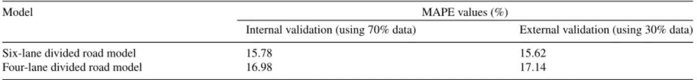
regression analysis. The models were validated both internally (using training data) and externally (using testing data). The models used 70% of collected data for training and rest 30% for testing. The Mean Absolute Percentage Error (MAPE) values for both models were less than the generally acceptable limit of 20% (Table 5).

Table 5. Validation results of models

Model MAPE values (%)

Internal validation (using 70% data) External validation (using 30% data)

Six-lane divided road model 15.78 15.62

Four-lane divided road model 16.98 17.14

6. Conclusions

The following ﬁndings and conclusions were evolved from the study:

1. The Free-ﬂow speeds (FFS) varies among various vehicle types. Subclasses within many of the vehicle classes exhibit diverse speed characteristics. Based on the collected data, mean FFS were observed to be highest for passenger cars (61 km/h), followed by light commercial vehicles (53 km/h), two-wheelers (48 km/h), buses (47 km/h), trucks (46 km/h) and three-wheelers (40 km/h). These are indicative of the FFS characteristics of heterogeneous traﬃc of urban roads in India.

2. The significant difference in FFS across vehicle groups suggests the need for inclusion of vehicle class (or subclass) as a factor in FFS models. This would help in understanding the variations in FFS with respect to variations in vehicle composition, which is an important characteristic of heterogeneous traffic.

3. Lane position is an important factor to be considered while estimating FFS on urban roads. FFS was found to be signiﬁcantly higher on inner lanes compared to the kerb lane.

4. FFS models for four- and six-lane divided urban roads show that roads factors such as carriageway width, link length, presence of kerb and landuse type are other signiﬁcant factors inﬂuencing FFS.

These are based on case study locations in Chennai, India. The findings point towards the need of understanding driver behaviour under heterogeneous traffic. The driver behaviour in India is believed to be different from those in several other countries. Here, many drivers tend to violate speed limits under low flow conditions. Drivers are also constrained by limitations of their vehicles, which may compel them to go slower. Also, it is believed that aggressiveness of certain large vehicle types influence these drivers to choose lanes that they consider preferable.

The present study deals with only divided urban roads. Urban roads also comprise of undivided roads which were not studied. Also, the present study is restricted to mid-block segments. Studying the inﬂuence of signalized intersec-tions may be instrumental in developing models to predict FFS of links and paths.The models could be expanded and improved by taking these aspects into consideration.

7. Acknowledgements

The support for this work by the Centre of Excellence in Urban Transport at IIT Madras, India, funded by the Ministry of Urban Development, Government of India, is gratefully acknowledged. The contributions of Mr. Sivakirubanandan and Mr. G. Arivazhagan during the data collection phase of the study are also acknowledged.

References

Bang, K.L., 1995. Impact of Side Friction on Speed-Flow Relationships for Rural and Urban Highways. Technical Report. SWEROAD Indonesia. Bandung, Indonesia.

De Luca, M., Lamberti, R., DellAcqua, G., 2012. Freeway Free Flow Speed: a Case Study in Italy, in: 15th Meeting of the EURO Working Group on Transportation, Paris, France. pp. 628–636.

(10)

Deardoﬀ, M.D., Wiesner, B.N., Fazio, J., 2011. Estimating Free-Flow Speed from Posted Speed Limit Signs, in: 6th International Symposium on Highway Capacity and Quality of Service, Stockholm , Sweden. pp. 306–316.

Dixon, K.K., Wu, C.H., Sarasua, W., Daniel, J., 1999. Posted and Free-Flow Speeds for Rural Multilane Highways in Georgia. Journal of Transportation Engineering 125, 487–494. doi:10.1061/(ASCE)0733-947X(1999)125:6(487).

Figueroa, A.M., Tarko, A.P., 2005. Speed Factors on Two-lane Rural Highways in Free-Flow Conditions. Transportation Research Record: Journal of the Transportation Research Board , 39–46.

Hablas, H.E., 2007. A Study of Inclement Weather Impacts on Freeway Free-Flow Speed. Master’s thesis. Virginia Polytechnic Institute and State University. Blacksburg, United States.

Himes, S., Donnell, E., 2010. Speed Prediction Models for Multilane Highways: Simultaneous Equations Approach. Journal of Transportation Engineering 136, 855–862. doi:10.1061/(ASCE)TE.1943-5436.0000149.

Kadiyali, L., Viswanathan, E., Gupta, R., 1983. Free Speeds of Vehicles on Indian Roads. Journal of Indian Road Congress 42.

Kyte, M., Khatib, Z., Shannon, P., Kitchener, F., 2000. Eﬀect of Environmental Factors on Free-Flow Speed, in: Fourth International Symposium on Highway Capacity, Maui, Hawaii. pp. 108–119.

Madhu, E., Velmurugan, S., Ravinder, K., Nataraju, J., 2011. Development of free-speed equations for assessment of road-user cost on high-speed multi-lane carriageways of India on Plain Terrain. Current Science 100, 1362–1372.

Moses, R., Mtoi, E., 2013. Evaluation of Free Flow Speeds on Interrupted Flow Facilities. Technical Report. Department of Civil Engineering, FAMU-FSU College of Engineering. Tallahassee, United States.

Qureshi, A.S., Khakheli, G.B., Memon, R.A., 2005. Operating Speed Prediction Model for Existing Two Lane Two-Way Old Alignments. Mehran University Research Journal of Engineering & Technology 24, 377–386.

R Development Core Team, 2008. R: A Language and Environment for Statistical Computing. R Foundation for Statistical Computing. Vienna, Austria. URL:http://www.R-project.org. ISBN 3-900051-07-0.

Shi, L.J., Cheng, Y., Ou, D.X., Chen, X.H., 2012. Modeling the Eﬀects of Rainfall on Urban Freeway Free-Flow Speeds. Applied Mechanics and Materials 178-181, 2577–2585.

Transportation Research Board, 2010. Highway Capacity Manual. Transportation Research Board, Washington DC, United States.

Yagar, S., Van Aerde, M., 1983. Geometric and Environmental Eﬀects on Speeds of Two-lane Highways. Transportation Research Part A: Policy and Practice 17A, 315–325.

Yusuf, I.T., 2010. The Factors For Free-Flow Speed On Urban Arterials Empirical Evidences From Nigeria. Journal of American Science 6, 1487–1497.