www.elsevier.com/locate/jspi
Improving predictive inference under covariate shift by
weighting the log-likelihood function
Hidetoshi Shimodaira
∗The Institute of Statistical Mathematics, 4-6-7 Minami-Azabu, Minato-ku, Tokyo 106-8569, Japan
Received 17 December 1998; received in revised form 21 January; accepted 25 February 2000
Abstract
A class of predictive densities is derived by weighting the observed samples in maximizing the log-likelihood function. This approach is eective in cases such as sample surveys or design of experiments, where the observed covariate follows a dierent distribution than that in the whole population. Under misspecication of the parametric model, the optimal choice of the weight function is asymptotically shown to be the ratio of the density function of the covariate in the population to that in the observations. This is the pseudo-maximum likelihood estima-tion of sample surveys. The optimality is dened by the expected Kullback–Leibler loss, and the optimal weight is obtained by considering the importance sampling identity. Under correct specication of the model, however, the ordinary maximum likelihood estimate (i.e. the uniform weight) is shown to be optimal asymptotically. For moderate sample size, the situation is in between the two extreme cases, and the weight function is selected by minimizing a variant of the information criterion derived as an estimate of the expected loss. The method is also applied to a weighted version of the Bayesian predictive density. Numerical examples as well as Monte-Carlo simulations are shown for polynomial regression. A connection with the robust parametric estimation is discussed. c 2000 Elsevier Science B.V. All rights reserved.
MSC: 62B10; 62D05
Keywords: Akaike information criterion; Design of experiments; Importance sampling; Kullback–Leibler divergence; Misspecication; Sample surveys; Weighted least squares
1. Introduction
Let x be the explanatory variable or the covariate, and y be the response variable. In predictive inference with the regression analysis, we are interested in estimating the conditional densityq(y|x) ofygivenx, using a parametric model. Let p(y|x; Â) be the model of the conditional density which is parameterized byÂ=(Â1; : : : ; Âm)0 ∈⊂Rm.
∗Correspondence address: Department of Statistics, Sequoia Hall, 390 Serra Mall, Stanford University,
Stanford, CA 94305-4065, USA.
E-mail address:[email protected] (H. Shimodaira).
0378-3758/00/$ - see front matter c2000 Elsevier Science B.V. All rights reserved. PII: S0378-3758(00)00115-4
Having observed i.i.d. samples of sizen, denoted by (x(n); y(n)) = ((x
t; yt): t= 1; : : : ; n),
we obtain a predictive densityp(y|x;ˆ) by giving an estimate ˆÂ= ˆÂ(x(n); y(n)). In this
paper, we discuss improvement of the maximum likelihood estimate (MLE) under both
(i) covariate shift in distribution and (ii) misspeciÿcation of the model as explained
below.
Let q1(x) be the density of x for evaluation of the predictive performance, while
q0(x) be the density of xin the observed data. We consider the Kullback–Leibler loss
function lossi(Â) := − Z qi(x) Z q(y|x)logp(y|x; Â) dydx
fori=0;1, and then employ loss1( ˆÂ) for evaluation of ˆÂ, rather than the usual loss0( ˆÂ).
The situation q0(x)6=q1(x) will be called covariate shift in distribution, which is one
of the premises of this paper.
This situation is not so odd as it might look at rst. In fact, it is seen in various elds as follows. In sample surveys,q0(x) is determined by the sampling scheme, whileq1(x)
is determined by the population. In regression analysis, covariate shift often happens because of the limitation of resources, or the design of experiments. In articial neural networks literature, “active learning” is the typical situation where we control q0(x)
for better prediction. We could say that the distribution of x in future observations is dierent from that of the past observations; xis not necessarily distributed as q1(x) in
future, but we can give imaginaryq1(x) to specify the region ofxwhere the prediction
accuracy should be controlled. Note that q0(x) and=or q1(x) are often estimated from
data, but we assume they are known or estimated reasonably in advance.
The second premise of this paper is misspecication of the model. Let ˆÂ0 be the
MLE of Â, and Â∗
0 be the asymptotic limit of ˆÂ0 as n → ∞. Under certain
regular-ity conditions, MLE is consistent and p(y|x; Â∗
0) =q(y|x) provided that the model is
correctly specied. In practice, however,p(y|x; Â∗
0) deviates more or less from q(y|x).
Under both the covariate shift and the misspecication, MLE does not necessarily provide a good inference. We will show that MLE is improved by giving a weight function w(x) of the covariate in the log-likelihood function
Lw(Â|x(n); y(n)):=− n
P
t=1lw(xt; yt|Â); (1.1)
wherelw(x; y|Â)=−w(x)logp(y|x; Â). Then the maximum weighted log-likelihood
esti-mate (MWLE), denoted by ˆÂw, is obtained by maximizing (1.1) over . It will be seen
that the weight functionw(x)=q1(x)=q0(x) is the optimal choice for suciently largen
in terms of the expected loss with respect toq1(x). We denote MWLE with this weight
function by ˆÂ1. A comparison between ˆÂ0 and ˆÂ1 is made in the numerical example of
polynomial regression of Section 2, and the asymptotic optimality of ˆÂ1 is shown in
Section 3. Note that MWLE turns out to be downweighting the observed samples which are not important in tting the model with respect to the population. An interpretation of MWLE as one of the robust estimation techniques is given in Section 9.
This type of estimation is not new in statistics. Actually, ˆÂ1 is regarded as a
gen-eralization of the pseudo-maximum likelihood estimation in sample surveys (Skinner et al., 1989, p. 80; Pfeermann et al., 1998); the log likelihood is weighted inversely proportional toq0(x), the probability of selecting unitx, whileq1(x) is equal probability
for all possible values ofx. The same idea is also seen in Rao (1991), where weighted maximum likelihood estimation is considered for unequally spaced time-series data.
The local likelihoods or the weighted likelihoods formally similar to (1.1) are found in the literature for semi-parametric inference. However, ˆÂw is estimated using a weight
function concentrated locally around each x or (x; y) in the semi-parametric approach; thus ˆÂw inp(y|x;ˆw) will depend on (x; y) as well as the data (x(n); y(n)). On the other
hand, we restrict our attention to a rather conventional parametric modeling approach here, and ˆÂw depends only on the data.
In spite of the asymptotic optimality ofw(x)=q1(x)=q0(x) mentioned above, another
choice of the weight function can improve the expected loss for moderate sample size by compromising the bias and the variance of ˆÂw. We develop a practical method for
this improvement in Sections 4–7. The asymptotic expansion of the expected loss is given in Section 4, and a variant of the information criterion is derived as an estimate of the expected loss in Section 5. This new criterion is used to nd a good w(x) as well as a good form of p(y|x; Â). The numerical example is revisited in Section 6, and a simulation study is given in Section 7.
In Section 8, we show the Bayesian predictive density is also improved by consid-ering the weight function. Finally, concluding remarks are given in Section 9. All the proofs are deferred to the appendix.
2. Illustrative example in regression
Here we consider the normal regression to predict the responsey∈R using a poly-nomial function of x∈R. Let the model p(y|x; Â) be the polynomial regression
y=ÿ0+ÿ1x+· · ·+ÿdxd+; ∼N(0; 2); (2.1)
whereÂ= (ÿ0; : : : ; ÿd; ) and N(a; b) denotes the normal distribution with mean a and
variance b. In the numerical example below, we assume the true q(y|x) is also given by (2.1) with d= 3:
y=−x+x3+; ∼N(0;0:32): (2.2)
The density q0(x) of the covariate x is
x∼N(0; 20); (2.3)
where0= 0:5, 20= 0:52. This corresponds to the sampling scheme ofx or the design
of experiments. A dataset (x(n); y(n)) of sizen= 100 is generated from (2.2) and (2.3),
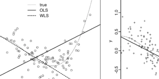
and plotted by circles in Fig. 1a. MLE ˆÂ0 is obtained by the ordinary least squares
(OLS) for the normal regression; we consider a model of the form (2.1) with d= 1, and the regression line tted by OLS is drawn in solid line in Fig. 1a.
Fig. 1. Fitting of polynomial regression with degreed= 1. (a) Samples (xt; yt) of sizen= 100 are generated fromq(y|x)q0(x) and plotted as circles, where the underlying true curve is indicated by the thin dotted line. The solid line is obtained by OLS, and the dotted line is WLS with weightq1(x)=q0(x). (b) Samples of
n= 100 are generated fromq(y|x)q1(x), and the regression line is obtained by OLS.
On the other hand, MWLE ˆÂw is obtained by weighted least squares (WLS) with
weights w(xt) for the normal regression. We again consider the model with d= 1,
and the regression line tted by WLS with w(x) =q1(x)=q0(x) is drawn in dotted line
in Fig. 1a. Here, the density q1(x) for imaginary “future” observations or that for the
whole population in sample surveys is specied in advance by
x∼N(1; 21); (2.4)
where1= 0:0; 21= 0:32. The ratio of q1(x) toq0(x) is
q1(x) q0(x)= exp(−(x−1)2=221)=1 exp(−(x−0)2=220)=0 ˙exp −(x−)2 2 2 ; (2.5) where 2= (−2 1 −−02)−1= 0:382, and = 2(1−21−0−20) =−0:28.
The obtained lines in Fig. 1a are very dierent for OLS and WLS. The question is: which is better than the other? It is known that OLS is the best linear unbiased estimate and makes small mean squared error of prediction in terms of q(y|x)q0(x)
which generated the data. On the other hand, WLS with weight (2.5) makes small prediction error in terms of q(y|x)q1(x) which will generate future observations, and
thus WLS is better than OLS here. To conrm this, a dataset of size n= 100 is generated from q(y|x)q1(x) specied by (2.2) and (2.4). The regression line of d= 1
tted by OLS is shown in Fig. 1b, which is considered to have small prediction error for the “future” data. The regression line of WLS tted to the past data in Fig. 1a is quite similar to the line of OLS tted to the future data in Fig. 1b. In practice, only the past data is available. The WLS gave almost the equivalent result to the future OLS by using only the past data.
The underlying true curve is the polynomial with d= 3, and thus the regression line of d= 1 cannot be tted to it nicely over all the region of x. However, the true curve is almost linear in the region of 1 ±21, and the nice t of the WLS
in this region is obtained by throwing away the observed samples which are outside of this region. The “eective sample size” may be dened in terms of the entropy by ne=exp(−Pnt=1ptlogpt), wherept=w(xt)=Pnt0=1w(xt0). In the WLS above,ne=49:3,
which is about the half of the original sample size n= 100, and then increases the variance of the WLS. This is discussed later in detail.
3. Asymptotic properties of MWLE
LetEi(·) denote the expectation with respect to q(y|x)qi(x) for i= 0;1. Considering
−Lw(Â) as the summation of i.i.d. random variables lw(xt; yt|Â), it follows from the
law of large numbers that −Lw(Â)=n→E0(lw(x; y|Â)) as n grows to innity. Then we
have ˆÂw →Â∗w in probability as n → ∞, where Âw∗ is the minimizer of E0(lw(x; y|Â))
overÂ∈. Hereafter, we restrict our attention to properw(x) such that E0(lw(x; y|Â))
exists for all Â∈and that the Hessian of E0(lw(x; y|Â)) is non-singular at Â∗w, which
is uniquely determined and interior to .
If the above result is applied to w(x) =q1(x)=q0(x), we nd that ˆÂ1 converges in
probability to the minimizer of loss1(Â) overÂ∈, which we denote Â1∗. Here the key
idea is the importance sampling identity: E0 q1(x) q0(x)logp(y|x; Â) = Z q(y|x)q0(x)qq1(x) 0(x)logp(y|x; Â) dxdy =E1(logp(y|x; Â)); (3.1)
which impliesE0(lw(x; y|Â))≡loss1(Â) and Âw∗=Â∗1 when w(x) =q1(x)=q0(x).
Except for the equivalent weight w(x)˙q1(x)=q0(x), we have Â∗w 6=Â∗1 under
mis-specication in general. From the denition of Â∗
1, therefore, loss1(Â∗w)¿loss1(Â∗1).
This immediately implies the asymptotic optimality of the weight w(x) =q1(x)=q0(x),
because ˆÂw→Â∗w and ˆÂ1→Â1∗ and thus loss1( ˆÂw)¿loss1( ˆÂ1) for suciently largen.
ˆ
Â1 has consistency in a sense that it converges to the optimal parameter value.
However, ˆÂ0 is more ecient than ˆÂ1 in terms of the asymptotic variance. This will
be important for moderate sample size, where n is large enough for the asymptotic expansions to be allowed, but not enough for the optimality of ˆÂ1to hold. The following
lemma, which is used in the subsequent sections, gives the asymptotic distribution of ˆ
Âw. The derivation is parallel to that of MLE under misspecication given in White
(1982); we replace logp(y|x; Â)q0(x) of MLE with w(x)logp(y|x; Â)q0(x) of MWLE. Lemma 1. Assume the regularity conditions similar to those of White (1982); i.e.;
the model is suciently smooth and the support of p(y|x; Â) is the same as that of
q(y|x) for all Â∈. Also assume Â∗
is asymptotically normally distributed as N(0; H−1
w GwHw−1); where Gw and Hw are
m×m matrices deÿned by Gw=E0 ( @lw(x; y|Â) @Â Â∗ w @lw(x; y|Â) @Â0 Â∗ w ) ; Hw=E0 ( @2l w(x; y|Â) @Â@Â0 Â∗ w ) ; (3.2)
which are assumed to be non-singular.
4. Expected loss
In the previous section, optimal choice ofw(x) was discussed in terms of the asymp-totic bias Â∗
w−Â∗1. For moderate sample size, however, the variance of ˆÂw due to
the sampling error should be considered. In order to take account of both the bias and the variance, we employ the expected loss E0(n)(loss1( ˆÂw)) to determine the
opti-mal weight; E0(n)(·) denotes the expectation with respect to (x(n); y(n)) which follows
Qn
t=1q(yt|xt)q0(xt).
Lemma 2. The expected loss is asymptotically expanded as
E0(n)(loss1( ˆÂw)) = loss1(Â∗w) +1n K[1] w 0bw+12tr(Kw[2]Hw−1GwHw−1) + o(n−1); (4.1)
where the elements of Kw[1] and Kw[2] are deÿned by
(K[k] w )i1···ik =−E0 ( q1(x) q0(x) @klogp(y|x; Â) @Âi1· · ·@Âik Â∗ w )
and bw is the asymptotic limit ofnE0(n)( ˆÂw−Â∗w); which is of order O(1).
The expression for bw is given in the following lemma. We use the summation
convention AiBi=Pmi=1AiBi in the formula.
Lemma 3. The elements of bw= limn→∞nE0(n)( ˆÂw−Âw∗) are given by
bi1
w:=Hwi1i2Hwj1j2{(Hw[2·1])i2j1·j2−12(Hw[3])i2j1k1Hwk1k2(Hw[1·1])k2·j2}; (4.2)
where Hwij denotes the (i; j) element of Hw−1; and
(H[k] w )i1···ik=E0 ( @kl w(x; y|Â) @Âi1· · ·@Âik Â∗ w ) ; (H[k·l] w )i1···ik·j1···jl=E0 ( @kl w(x; y|Â) @Âi1· · ·@Âik Â∗ w @ll w(x; y|Â) @Âj1· · ·@Âjl Â∗ w ) :
For suciently large n, loss1(Âw∗) is the dominant term on the right-hand side of
(4.1), and the optimal weight is w(x) =q1(x)=q0(x) as seen in Section 3. If n is not
large enough compared with the extent of the misspecication, the O(n−1) terms related
to the rst and second moments of ˆÂw−Â∗w cannot be ignored in (4.1), and the optimal
weight changes. In an extreme case where the model is correctly specied, we only have to look at the O(n−1) terms as shown in the following lemma.
Lemma 4. Assume there exists Â∗∈ such thatq(y|x) =p(y|x; Â∗). Then; Â∗ w=Â∗ and q(y|x) =p(y|x; Â∗
w) for all proper w(x). The expected loss E0(n)(loss1( ˆÂw)) is
minimized when w(x)≡1 for suciently large n.
5. Information criterion
The performance of MWLE for a specied w(x) is given by (4.1). However, we cannot calculate the value of the expected loss from it in practice, because q(y|x) is unknown. We provide a variant of the information criterion as an estimate of (4.1).
Theorem 1. Let the information criterion for MWLE be
ICw:=−2L1( ˆÂw) + 2 tr(JwHw−1); (5.1) where L1(Â) = n P t=1 q1(x) q0(x)logp(yt|xt; Â); Jw=−E0 ( q1(x) q0(x) @logp(y|x; Â) @ Â∗ w @lw(x; y|Â) @Â0 Â∗ w ) :
The matrices Jw and Hw may be replaced by their consistent estimates
ˆ Jw=−1n n P t=1 q1(xt) q0(xt) @logp(yt|xt; Â) @ Â ˆ Âw @lw(xt; yt|Â) @Â0 ˆ Âw ; ˆ Hw=1n n P t=1 @2l w(xt; yt|Â) @Â@Â0 ˆ Âw :
Then; ICw=2n is an estimate of the expected loss unbiased up to O(n−1) term:
E0(n)(ICw=2n) =E0(n)(loss1( ˆÂw)) + o(n−1): (5.2)
Fortunately, expression (5.1) turns out to be rather simpler than that of (4.1), and we do not have to worry about the calculation of the third derivatives appeared in (4.2). The explicit form of (5.1) for the normal regression is given in (6.1) and (6.2). Given the modelp(y|x; Â) and the data (x(n); y(n)), we choose a weight functionw(x)
which attains the minimum of ICw over a certain class of weights. This is selection
possible forms ofw(x) is equivalent ton-dimensional optimization problem with respect to (w(xt): t= 1; : : : ; n). But we do not take this line here, because of the computational
cost as well as a conceptual diculty which will be mentioned in Section 9. Rather than the global search, we shall pick a better one from the two extreme cases of w(x)≡1 and w(x) =q1(x)=q0(x), or consider a class of weights by connecting the two
extremes continuously: w(x) = q1(x) q0(x) ; ∈[0;1]; (5.3)
where = 0 corresponds to ˆÂ0 and = 1 corresponds to ˆÂ1. In the next section, we
numerically nd ˆ which minimizes ICw by searching over∈[0;1]. Note that (5.3) is
proportional to N( ;2=) in the case of (2.5), and−1=2 is the window scale parameter.
When we have several candidate forms of p(y|x; Â), the model and the weight are selected simultaneously by minimizing ICw. A similar idea of the simultaneous
selection is found in Shibata (1989), where an information criterion RIC is derived for the penalized likelihood. A crucial distinction, however, is that the weight for  is selected in RIC, whereas the weight for x is selected in ICw. Another distinction is
that the weight is additive to the log likelihood in RIC, while it is multiplicative in ICw.
Akaike (1974) gave an information criterion
AIC =−2L0( ˆÂ0) + 2 dimÂ; (5.4)
whereL0(Â) is the log-likelihood function. AIC is intended for MLE, and it is obtained
as a special case of ICw. When q1(x) =q0(x) and w(x)≡1, ICw reduces to
TIC =−2L0( ˆÂ0) + 2 tr(G0H0−1);
where G0=Gw and H0=Hw when w(x)≡1. TIC is derived by Takeuchi (1976) as
a precise version of AIC, and it is equivalent to the criterion of Linhart and Zucchini (1986). Ifp(y|x; Â∗
0) is suciently close toq(y|x), tr(G0H0−1)≈dimÂand TIC reduces
to AIC.
6. Numerical example revisited
For the normal linear regression, such as the polynomial regression given in (2.1), ÿ-components of ˆÂw are obtained by WLS with weights w(xt). -component of ˆÂw is
then given by ˆ2=Pnt=1w(xt) ˆ2t=cˆw, where ˆcw =Pnt=1w(xt) and ˆt is the residual.
Letting ˆht, t= 1; : : : ; n be the diagonal elements of the hat matrix used in the WLS,
the information criterion (5.1) is calculated from
−L1( ˆÂw) =12 n P t=1 q1(xt) q0(xt) ( ˆ 2 t ˆ 2 + log(2ˆ 2) ) ; (6.1)
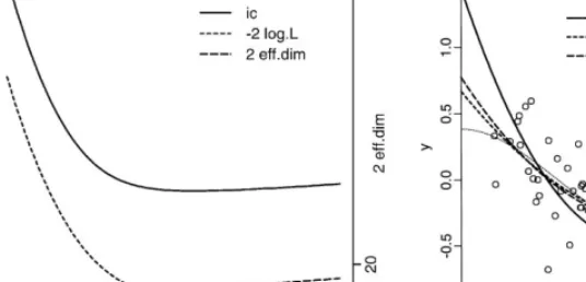
Fig. 2. (a) Curve of ICwversus∈[0;1] for the model of Section 2 withd= 2. The weight function (5.3)
connecting fromw(x)≡1 (i.e.=0) tow(x)=q1(x)=q0(x) (i.e.=1) was used. Also shown are−2L1( ˆÂw) in dotted lines, and 2 tr(JwH−1
w ) in broken lines. (b) The regression curves ford= 2. The WLS curve with
the optimal ˆas well as those for OLS (= 0) and WLS (= 1) are drawn. Table 1
ICwvalues with weight (5.3) for=0,=1, and= ˆ. Also shown is ˆvalue. Calculated for the polynomial
regression example of Section 2 withd= 0; : : : ;4
d= 0 d= 1 d= 2 d= 3 d= 4 = 0 138.72 174.02 63.59 28.97 31.75 = 1 73.96 33.23 33.64 34.80 34.98 = ˆ 73.92 32.68 32.62 28.96 31.75 ˆ 0.95 0.77 0.56 0.01 0.00 tr( ˆJwHˆ−w1) = n P t=1 q1(xt) q0(xt) ˆ 2 t ˆ 2hˆt+ w(xt) 2 ˆcw ˆ 2 t ˆ 2 −1 !2 : (6.2)
We apply the above formulas to the data generated from (2.2) and (2.3) in Section 2. Fig. 2a shows the plot of the information criterion and its two components ford= 2. By increasing from 0 to 1, the rst term of (5.1) decreases while the second term increases in general. We numerically nd ˆ so that the two terms balance. For d= 2, ICw takes the minimum 32.62 at ˆ = 0:56. The regression curves obtained by this
method are shown in Fig. 2b.
Table 1 shows ICw values for d= 0; : : : ;4. For each d, ICw is minimized at = ˆ.
Then, ICw of ˆ is minimized at the model d= 3. By minimizing ICw, and d are
simultaneously selected. For d= 3, it turns out that ˆ= 0:01≈0. In fact, the model of d= 3 is correctly specied in this dataset, and it follows from Lemma 4 that ˆÂ0 is
optimal ford¿3. Even in such a situation, the appropriate ˆis selected by minimizing ICw.
Table 2
Asymptotic convergence of the second term of (4.1). 2n times of loss1( ˆÂw)−loss1(Â∗w) is calculated for
the Monte-Carlo replicates, and its average is tabulated. For every simulation (d= 0;1;2 and= 0;1), the values are showing a good convergence asn→ ∞
n d= 0 d= 1 d= 2 = 0 = 1 = 0 = 1 = 0 = 1 50 −3.9 5.5 −2.0 8.9 19.0 15.9 100 −5.1 4.8 −3.1 7.6 17.7 11.3 300 −7.0 4.5 −4.5 6.8 17.7 9.0 1000 −8.0 4.4 −4.9 6.6 19.3 8.5 Table 3
Asymptotic convergence of (5.2). 2nloss1( ˆÂw)+2L1( ˆÂw) is calculated for the Monte-Carlo replicates, and its average is tabulated in the left columns. Forn¿300, this agrees very well with the average of 2 tr( ˆJwHˆ−w1)
tabulated in the right columns. 2 tr(JwH−1
w ) is shown in then=∞row
n d= 0 d= 1 d= 2 = 0 = 1 = 0 = 1 = 0 = 1 50 1.8 1.7 9.9 7.7 6.8 6.1 15.7 11.1 26.4 13.1 24.8 13.4 100 1.5 1.4 9.2 8.1 6.0 5.7 14.2 12.0 22.6 14.9 19.8 14.9 300 1.3 1.3 8.8 8.4 5.4 5.3 13.3 12.6 18.5 15.7 17.3 16.0 1000 1.2 1.2 8.7 8.6 5.1 5.1 13.1 12.9 16.2 15.4 16.7 16.3 ∞ 1.2 8.6 5.0 13.0 14.9 16.4
In practical data analysis, it would be rare to have correctly specied models at hand. Therefore, we excluded¿3 from the above example, and restrict the candidates to d ¡3. Then, d= 2 is selected, and d= 1 has almost the same ICw value, while
d= 0 has signicantly larger ICw value. This agrees with the asymptotic result veried
by extensive Monte-Carlo simulations in Shimodaira (1997) that (4.1) is minimized when = 1 and d= 1 over d∈ {0;1;2}, for suciently large n.
7. Simulation study
First we show simulation results in Tables 1–3 which conrm the theory of Sections 4 and 5. A large number N of replicates of the dataset of size n are generated from (2.2) and (2.3). We used (2.4) as q1(x). Four simulations of n= 50, 100, 300, and
1000 are done with N = 105 for n= 50–300 and N = 106 for n= 1000. For each
replicate of the dataset, ˆÂw is calculated for = 0;1 and d= 0;1;2. Then, loss1( ˆÂw),
L1( ˆÂw), and tr( ˆJwHˆ−w1) are calculated, and their averages over the N replicates are
obtained for each simulation. The tables show nice agreement between the simulations and the theory.
Next, we show the results of another set of simulations in Table 4 which conrms the practical performance of the weight selection procedure. We used (2.3) and (2.4) as before, but (2.2) is replaced by y=−x+ÿ3x3+ for generating replicates of the
Table 4
The expected loss for the selected weight and the selected model. 2n times of loss1( ˆÂw) +E1(logq(y|x)) is calculated for the replicates, and its average is tabulated in the columns of = 0;1 ford= 0;1;2. The average of the loss of the selected weight is shown in the columns of ˆ. The right most columns show the average of the loss of the selected model
ÿ3 d= 0 d= 1 d= 2 dˆ 0 1 ˆ 0 1 ˆ 0 1 ˆ 0 1 ˆ 1.0 98.0 50.7 50.9 123.8 12.3 11.9 71.7 16.0 16.7 73.2 15.0 15.3 0.5 96.0 61.1 61.1 49.9 9.0 8.2 25.6 11.8 11.5 26.9 11.0 10.8 0.2 142.2 68.4 68.4 12.6 7.8 6.4 8.5 10.4 8.1 10.1 9.6 7.9 0.1 152.8 71.1 71.0 6.0 7.8 5.7 5.9 10.4 7.2 6.3 9.6 6.9 0.0 162.2 73.8 73.7 3.6 7.7 4.8 5.0 10.2 6.6 4.4 9.5 6.0
dataset of sizen=100. Five simulations ofÿ3=1:0, 0.5, 0.2, 0.1, and 0.0 are done with
N=104. In the table,E1(−logq(y|x)) is subtracted from the loss to make comparisons
easier.
The expected loss of MLE (= 0) is 123.8 forÿ3= 1:0,d= 1, while that of MWLE
(= 1) is 12.3, showing a great improvement as we have observed in the numerical example. The expected loss of MWLE with the selected weight ( ˆ) is 11.9, which is not signicantly dierent from that of = 1. This is a consequence of the large sample size n= 100, where the rst term of (4.1) or (5.1) is dominant. The same observation holds for ÿ3= 1:0–0:0, d= 0, andÿ3= 1:0;0:5, d= 1;2.
On the other hand,=0 is signicantly better than=1 forÿ3=0:0,d=1;2, where
the model is correctly specied. In this case the second term of (4.1) is dominant and = 0 is the optimal choice as mentioned in Lemma 4. The selected weight ˆ performs close to = 0, but with slightly larger expected loss. This dierence is the price we pay for the weight selection using (5.1) which is an estimate of (4.1), not the true value of (4.1).
For all the cases of ÿ3= 1:0–0.0, d= 0;1;2, the weight selection procedure gives
the expected loss close to the optimal choice. Fixing to either of 0 or 1 can lead to very poor performance. The same observation holds for the model selection as shown in the columns of ˆd.
8. Bayesian inference
We have been working on the predictive density
p(y|x;ˆw); (8.1)
which is based on MWLE ˆÂw. This type of predictive density is occasionally called
as an estimative density in the literature. Another possibility is the Bayesian predictive density. Here we consider a weighted version of it, and examine its performance in prediction.
Let p(Â) be the prior density of Â. Given the data (x(n); y(n)), we shall dene the
weighted posterior density by
pw(Â|x(n); y(n))˙p(Â)expLw(Â|x(n); y(n)): (8.2)
Then the predictive density will be pw(y|x; x(n); y(n)) =
Z
p(y|x; Â)pw(Â|x(n); y(n)) dÂ: (8.3)
In the case of w(x) ≡ 1, (8.2) reduces to the ordinary posterior density, and (8.3) reduces to the ordinary Bayesian predictive density.
The Kullback–Leibler loss of (8.3) with respect to q(y|x)q1(x) is
−
Z
q1(x)
Z
q(y|x)logpw(y|x; x(n); y(n)) dydx
and thus the expected loss is given by
E0(n)(E1(−logpw(y|x; x(n); y(n)))): (8.4)
Lemma 5. For suciently large n; (8:4)is asymptotically expanded as
E0(n)(loss1( ˆÂw)) + 1n K[1] w 0aw−12tr((Kw[1·1]−Kw[2])Hw−1) + o(n−1); (8.5) where K[1·1] w =E0 ( q1(x) q0(x) @logp(y|x; Â) @ Â∗ w @logp(y|x; Â) @Â0 Â∗ w )
and aw= plimn→∞aˆw is the probability limit of
ˆ aw=n
Z
(Â−ˆw)pw(Â|x(n); y(n)) dÂ:
Furthermore; (8:4) is estimated by an information criterion
−2Pn t=1 q1(xt) q0(xt)logpw(yt|xt; x (n); y(n)) + 2 tr(J wHw−1): (8.6)
In fact; the expectation of (8:6); if divided by 2n; is equal to (8:5) up to O(n−1)
terms.
When q1(x) =q0(x) and w(x) ≡ 1, (8.6) reduces to the information criterion for
the Bayesian predictive density given in Konishi and Kitagawa (1996). Selection of w(x) as well as selection ofp(Â) andp(y|x; Â) becomes possible by minimizing (8.6). Comparing the values of (5.1) and (8.6), we can also choose which to use from (8.1) and (8.3).
The decrease of the expected loss of (8.3) from that of (8.1) is of order O(n−1) as
shown in (8.5), which can be positive or negative depending on q(y|x). For brevity sake, we assume q1(x) =q0(x) andw(x)≡1 below. Then the decrease in the expected
loss is =2n+ o(n−1), where = (tr(G
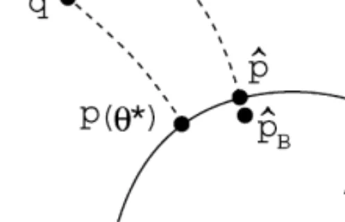
Fig. 3. The curvature of the model in relation to the location of the true densityq. On the parametric model denoted byp(·), we have= 0, and||increases asqdeviates fromp(·). The region of ¿0 is in the inside direction of the model, and ¡0 is in the outside direction of the model. ˆqdenotes the empirical distribution, and the projection of ˆqto the model is the estimative density ˆp=p(y|x;ˆ0). ˆpB denotes the Bayesian predictive density.
misspecication in general, which is utilized in the information matrix tests (White, 1982) for detecting the misspecication.
An enlightening interpretation of may be possible by the following geometric argument using the terminology of Efron (1978) and Amari (1985). Fig. 3 shows the space of all conditional densities. is determined by the extent of the misspecication multiplied by the “embedding mixture curvature” of the model (S. Amari, personal communication). Bayesian predictive density ˆpB is a mixture of p(y|x; Â) around ˆÂ0,
and thus it is located in the inside of the model because of the curvature; ˆpB deviates from ˆpof order O(n−1) as shown in Davison (1986). Therefore, ˆp
Bhas larger expected
loss than ˆp if q(y|x) is located in the outside of the model (i.e. ¡0), because ˆpB is located in the opposite side of q. This does not contradict the classical result that the expected loss of ˆpB is asymptotically smaller than that of ˆp for some prior. In Bayesian literature, the case of correct specication (i.e. = 0) is discussed and the dierence of the expected loss is of order O(n−2) as seen in Komaki (1996). Note
that the quadratic form of is relevant when the curvature vanishes, and ¿0 if all the eigenvalues are non-negative; see Shimodaira (1997) for details.
9. Concluding remarks
Although the ratio q1(x)=q0(x) has been assumed to be known, it is often estimated
from data in practice. Assuming q1(x) is known, we tried three possibilities in the
numerical example of Section 2: (i) q0(x) is specied correctly without unknown
pa-rameters. (ii) Assuming the normality of q0(x), the unknown 0 and 0 are estimated.
(iii) Non-parametric kernel density estimation is applied to q0(x). Then, it turns out
that MWLE is robust against the estimation of q1(x)=q0(x) and the results are almost
identical in the three cases. This may be because the form ofq0(x) is quite simple and
A parametric approach to take account of estimation of q1(x)=q0(x) is considered as
follows. Let the observed datazt; t=1; : : : ; n, followp0(z|Â), while future observations
will follow p1(z|Â). Then a possible estimating equation will be
n
P
t=1w(zt|Â)
@logp1(zt|Â)
@Â = 0; (9.1)
where w(z|Â) = (p1(z|Â)=p0(z|Â)). The solution of (9.1) reduces to the MWLE
dis-cussed in this paper by letting z = (x; y); p0(z|Â) =p(y|x; Â)q0(x), and p1(z|Â) =
p(y|x; Â)q1(x).
The estimating equation (9.1) is often seen in the literature of the robust parametric estimation; e.g., Green (1984), Hampel et al. (1986), Lindsay (1994), Basu and Lindsay (1994), Field and Smith (1994) and Windham (1995). In this context, the samples which are not concordant to the model p1(z|Â) will be regarded as “outliers” and
downweighted to reduce the impact on the parameter estimation. The specication of the weight function is thus the focal point of the argument. Although the covariate shift is a mechanism dierent from the outliers, an interpretation of MWLE in terms of the robust estimation can be given as follows. For simplicity, let z be a discrete random variable and ˆp0(z) be the observed relative frequency which estimates the contaminated distribution p0(z) consistently. The weight (p1(z|Â)=pˆ0(z)) in (9.1) then leads to the
minimum disparity estimator obtained by minimizing the power divergence 2nI−= 2 (−1) P z pˆ0(z) ( ˆ p0(z) p1(z|Â) − −1 )
(Cressie and Read, 1984; Lindsay, 1994). The uniform weight = 0 is sensitive to outliers, and a positive value = 0:5, say, improves the robustness. In the regression analysis, the deviation of p0(z) from p1(z) is decomposed into two parts: the
mis-specication of p(y|x; Â) and the covariate shift. MWLE is obtained by applying the power weighting scheme to the second part where = 1 is asymptotically optimal. It may be interesting to consider a robust version of MWLE by applying the weight, say (p1(y|x; Â)=pˆ0(y|x)) with = 0:5, to the rst part as well.
A numerical example of simultaneous selection of the weight and the model by the information criterion is shown in Section 6. The information criterion takes account of the selection bias caused by estimation of the parameter, but it does not take account the bias caused by the selection of the weight and the model. It is important to evaluate the expected loss of the predictive density obtained after these selection. The simulation study of Section 7 indicates that the method presented in this paper is eective, and the nal expected loss of the selected weight and=or model is reasonably small.
Although we have employed a specic type of one-parameter connection in (5.3), other types of connection may work similarly. However, increasing the number of con-nection parameters will increase the nal expected loss because of the sampling error of (5.1) as an estimator of (4.1). We observed the slight increase of the expected loss of ˆ in Table 4, and this increase can be much larger for multi-parameter connections.
We derived a variant of AIC for MWLE under covariate shift. On the other hand, Shimodaira (1994) and Cavanaugh and Shumway (1998) discussed variants of AIC for MLE in the presence of incomplete data. Information criteria have to be tailored for dierent styles of sampling scheme, and the unied approach for them is left as a future work.
A software for calculating ICw and ˆ of normal regression will be available in S
language at http://www.ism.ac.jp/˜shimo/.
Acknowledgements
I would like to thank John Copas, Tony Hayter, Motoaki Kawanabe, Shinto Eguchi, and the reviewers for helpful comments and suggestions.
Appendix A.
Proof of Lemma 1. Since Â∗
w is interior to, so is ˆÂw for suciently largen. Then,
ˆ
Âw is obtained as a solution of the estimating equation n P t=1 @lw(xt; yt|Â) @Â ˆ Âw = 0: (A.1)
The Taylor expansion of (A.1) leads to n−1Pn t=1 @2l w(xt; yt|Â) @Â@Â0 Â∗ w n1=2( ˆÂ w−Â∗w) =−n−1=2 n P t=1 @lw(xt; yt|Â) @ Â∗ w + Op(n−1=2): (A.2) It follows from the central limit theorem that the right-hand side is asymptotically distributed as N(0; Gw), while the left-hand side converges to Hwn1=2( ˆÂw−Â∗w). Thus
we obtained the desired result.
Proof of Lemma 2. The Taylor expansion of loss1( ˆÂw) aroundÂ∗w is
loss1(Â∗w) +1n (K[1] w )in1=2Â˙iw+12(Kw[2])ijÂ˙iwÂ˙jw + Op(n−3=2); (A.3)
where ˙Âw= n1=2( ˆÂw−Âw∗), and the summation convention AiBi=Pmi=1AiBi is used.
Considering Lemma 1, the expectation of (A.3) gives (4.1). By taking expectation of (A.2), we observe bw= O(1).
Proof of Lemma 3. Considering the Op(n−1=2) term in (A.2) explicitly, the Taylor
expansion of (A.1) gives ˆ H∗wÂ˙w=−n−1=2 n P t=1 @lw(xt; yt|Â) @Â Â∗ w +n−1=2e w;
where ˆ H∗w=1nPn t=1 @2lw(xt; yt|Â) @Â@Â0 Â∗ w ; (ew)i=−12(Hw[3])ijkÂ˙jwÂ˙kw+ Op(n−1=2): Noting ˆH∗−w 1=H−1 w −Hw−1( ˆHw∗−Hw)Hw−1+ Op(n−1); n1=2E0(n)( ˙Âw) is written as E0 H−1 w @ 2l w(x; y|Â) @Â@Â0 Â∗H −1 w @lw(@Âx; y|Â) Â∗ +H−1 w E0(n)(ew) + O(n−1=2);
which immediately implies (4.2).
Proof of Lemma 4. For any x, the conditional Kullback–Leibler loss loss(Â|x) =−
Z
q(y|x)logp(y|x; Â) dy
is minimized at Â∗ if q(y|x) =p(y|x; Â∗). Then Â∗
w =Â∗ for any w(x), because
E0(lw(x; y|Â)) =Rq(x)w(x)loss(Â|x) dx. Thus loss1(Â∗w) in (4.1) is equal for anyw(x).
Considering Kw[1]= 0, the second term in (4.1) is written as
n−1tr(K[2]
w Q(w)−1Q(w2)Q(w)−1); (A.4)
whereKw[2]=Q(q1=q0) andQ(a) is dened for anya(x) by
Q(a) =E0 a(x) @logp@Â(y|x; Â) Â∗ @logp(y|x; Â) @Â0 Â∗ :
It it easy to verify that Q(w)−1Q(w2)Q(w)−1−Q(1)−1 is non-negative denite for
any w(x), and so (A.4) is minimized when w(x)≡1.
Proof of Theorem 1. The Taylor expansion of logp(y|x;ˆw) aroundÂ∗w gives
L1( ˆÂw) =L1(Â∗w) +1n ( @L1(Â) @Â0 Â∗ w n1=2Â˙ w+12 @ 2L1(Â) @Âi@Âj Â∗ w ˙ ÂiwÂ˙jw ) + Op(n−1=2)
and thus E(0n)(−L1( ˆÂw)=n) is expanded as
loss1(Â∗w)−1nE0(n) ( 1 n @L1(Â) @Â0 Â∗ w n1=2Â˙ w ) +21ntr(K[2] w Hw−1GwHw−1) + O(n−3=2): (A.5) Considering −n−1@L1(Â)=@Â|Â∗ w=K [1]
w + Op(n−1=2), the second term of (A.5) becomes
1 nKw[1]0bw+1nE0(n) ( n1=2 −1 n @L1(Â) @Âi Â∗ w −(K[1] w )i ! ×Hij w n−1=2 @L@Âw(jÂ) Â∗ w + Op(n−1=2) !) =1 nKw[1]0bw− 1 nHwij(Jw)ij+ O(n−3=2):
Proof of Lemma 5. Assuming certain regularity conditions similar to those of Johnson (1970), we have the asymptotic limit of (8.2) is normal with mean ˆÂw and covariance
matrix ˆH−w1=n, since logpw(Â|x(n); y(n)) is expanded as
−1
2n1=2(Â−ˆw)0Hˆwn1=2(Â−ˆw) + Op(n−1=2);
where the terms independent of are omitted. Then, (8.3) is asymptotically expanded as p(y|x;ˆw) +n1 @p(@Ây|x; Â0 ) ˆ Âw ˆ aw+21ntr @ 2p(y|x; Â) @Â@Â0 ˆ Âw ˆ H−w1 ! + op(n−1): (A.6)
Note that Dunsmore (1976) gave the unweighted version of (A.6) when the model specication is correct, but the term of ˆaw was missing as indicated by Komaki (1996).
Applying the identity 1 p @2p @Â@Â0 = @logp @Â @logp @Â0 + @2logp @Â@Â0
to the third term of (A.6), we obtain logpw(y|x; x(n); y(n)) =logp(y|x;ˆw) +1n @logp@Â(y0|x; Â) Â∗ w aw+21ntr ( @logp(y|x; Â) @ Â∗ w × @logp(y|x; Â) @Â0 Â∗ w + @2logp(y|x; Â) @Â@Â0 Â∗ w ! H−1 w ) + op(n−1): (A.7)
Thus (8.5) immediately follows from (A.7). The last statement of the lemma is veried by combining (A.7) with Theorem 1.
References
Akaike, H., 1974. A new look at the statistical model identication. IEEE Trans. Automat. Control 19, 716–723.
Amari, S., 1985. Dierential-Geometrical Methods in Statistics. Lecture Notes in Statistics, Vol. 28. Springer, Berlin.
Basu, A., Lindsay, B.G., 1994. Minimum disparity estimation for continuous models: eciency, distributions and robustness. Ann. Inst. Statist. Math. 46, 683–705.
Cavanaugh, J.E., Shumway, R.H., 1998. An Akaike information criterion for model selection in the presence of incomplete data. J. Statist. Plann. Infererence 67, 45–65.
Cressie, N., Read, T.R.C., 1984. Multinomial goodness-of-t tests. J. Roy. Statist. Soc. Ser. B 46, 440–464. Davison, A.C., 1986. Approximate predictive likelihood. Biometrika 73, 323–332.
Dunsmore, I.R., 1976. Asymptotic prediction analysis. Biometrika 63, 627–630. Efron, B., 1978. The geometry of exponential families. Ann. Statist. 6, 362–376.
Field, C., Smith, B., 1994. Robust estimation – a weighted maximum likelihood approach. Internat. Statist. Rev. 62, 405–424.
Green, P.J., 1984. Iteratively reweighted least squares for maximum likelihood estimation, and some robust and resistant alternatives (with discussion). J. Roy. Statist. Soc. Ser. B 46, 149–192.
Hampel, F.R., Ronchetti, E.M., Rousseeuw, P.J., Stahel, W.A., 1986. Robust Statistics: The Approach Based on Inuence Functions. Wiley, New York.
Johnson, R.A., 1970. Asymptotic expansions associated with posterior distributions. Ann. Math. Statist. 41, 851–864.
Komaki, F., 1996. On asymptotic properties of predictive distributions. Biometrika 83, 299–313.
Konishi, S., Kitagawa, G., 1996. Generalised information criteria in model selection. Biometrika 83, 875–890. Lindsay, B.G., 1994. Eciency versus robustness: the case for minimum Hellinger distance and related
methods. Ann. Statist. 22, 1081–1114.
Linhart, H., Zucchini, W., 1986. Model Selection. Wiley, New York.
Pfeermann, D., Skinner, C.J., Holmes, D.J., Goldstein, H., Rasbash, J., 1998. Weighting for unequal selection probabilities in multilevel models. J. Roy. Statist. Soc. Ser. B 60, 23–56.
Shibata, R., 1989. Statistical aspects of model selection. In: Willems, J.C. (Ed.), From Data to Model. Springer, Berlin, pp. 215–240.
Shimodaira, H., 1994. A new criterion for selecting models from partially observed data. In: Cheeseman, P., Oldford, R.W. (Eds.), Selecting Models from Data: AI and Statistics IV. Springer, Berlin, pp. 21–30 (Chapter 3).
Shimodaira, H., 1997. Predictive inference under misspecication and its model selection. Research Memorandum 642, The Institute of Statistical Mathematics, Tokyo, Japan.
Skinner, C.J., Holt, D., Smith, T.M.F., 1989. Analysis of Complex Surveys. Wiley, New York.
Takeuchi, K., 1976. Distribution of information statistics and criteria for adequacy of models. Math. Sci. (153), 12–18 (in Japanese).
White, H., 1982. Maximum likelihood estimation of misspecied models. Econometrica 50, 1–26. Windham, M.P., 1995. Robustifying model tting. J. Roy. Statist. Soc. Ser. B 57, 599–609.