Does R&D spur productivity growth in Australia’s broadacre agriculture?
A semi-parametric smooth coefficient approach
Farid Khan
Department of Economics, University of Rajshahi
Email: faridecoru@yahoo.co.uk; Cell: +88 01712 208970
Ruhul Salim*
School of Economics and Finance, Curtin University Email: Ruhul.Salim@cbs.curtin.edu.au
Kai Sun
Salford Business School, University of Salford
Email: ksun1@binghamton.edu or ksun1@shu.edu.cn
Acknowledgement: Authors are grateful to thediscussantand participants in the 2014 Asia-Pacific Productivity Conference at the University of Queensland and Professor Subal Kumbhakar of Binghamton University, New York for helpful comments and suggestions. They are also thankful to the John Curtin Emirates Professor Harry Bloch, Dr Nazrul Islam from Curtin University and Professor Chris O’Donnell from the University of Queensland for their comments on the earlier drafts.
* Corresponding author:
Corresponding author: Associate Professor Ruhul Salim, School of Economics & Finance, Curtin University, Perth, WA, 6845. Phone: +618 9266 4577, E-mail: Ruhul.Salim@cbs.curtin.edu.au
Does R&D spur productivity growth in Australia’s broadacre agriculture?
A semi-parametric smooth coefficient approach
Abstract
This article analyses the role of research and development (R&D) in Australia's broadacre farming by using the semi-parametric smooth coefficient model proposed by Li et al. (2002). While the conventional production function approach only captures the direct effects of R&D, this methodology captures both the direct impact of a change in R&D on output and the indirect impact through changes in efficiency of use of factor inputs in the production process. Moreover, technical inefficiency is introduced in the model allowing it as a function of R&D. Using a unique state-level dataset covering the period 1995-2007, this empirical study finds that once both the direct and indirect effects are taken into consideration, R&D investments significantly increase outputs. The results also show that there are substantial variations in the effects of R&D on output across the state-level average farm through technology parameters as well as through technical inefficiency. Such variations need to be taken into account when designing policies for investing public R&D in agriculture.
Keywords: Broadacre Agriculture, Semi-parametric smooth coefficient model, Productivity, Research and Development
JEL Classification: C14, C23, D24
1. Introduction
There has been a recent concern that the productivity growth in agriculture is slowing in developed countries (Ball et al., 2013; Khan et al. 2014). Particularly, in Australia, an evidence of a slowdown in productivity growth over the last decade compared with earlier periods is revealed in at least some sectors of Australian agriculture (Khan et al. 2014; Sheng et al. 2015). Falling productivity has implications for domestic food security and rural livelihoods as well as for the food security in developing countries, where growing populations will continue to increase their demand for food in the coming decades (Pardey et al. 2006). Studies suggest that one of the primary reasons for slowing productivity growth in agriculture is that public investment in research and development (here after R&D) has been declining over the past few decades (Mullen 2010; Pardey et al. 2013; Suphannachart and Warr 2011). In particular, the sluggishness in public R&D since the mid-1970s in Australia may have contributed to the slowdown in agricultural productivity growth in recent periods in the country (Mullen 2010).
These recent phenomena in agriculture have rekindled interest in investigating the relationship between public funding in agricultural R&D and productivity.
The role of public R&D in productivity has been recognized since the early studies of agricultural economics. For example, Schultz (1953) estimates the returns to public R&D and attributes all of the productivity growth in agriculture to public investments in agricultural research. Similarly, Griliches (1964) estimates the Cobb-Douglas type agricultural production function while introducing a research and extension variable along with the conventional input variables. The investment in agricultural R&D is one of the leading factors that fuels productivity improvements in agriculture producing new knowledge and achieving technological breakthroughs (Alene 2010; Coe and Helpman 1995; Griliches 1988; Mullen, Scobie and Crean 2008; Wang et al. 2013). It leads to a more effective use of existing resources and thereby increases productivity levels.
The contribution of R&D expenditure to farm productivity growth is also evident in Australian agriculture, which is primarily based on extensive cropping and livestock farming activity and generally termed as ‘broadacre’ agriculture. Broadacre agriculture is a significant contributor to the country’s agricultural and economic growth. It generates more than 54 per cent of the country’s gross value of agricultural production (Gray et al. 2014). Moreover, Australia exports approximately 60 per cent of its agricultural production, accounting for 10.9 per cent of the total export earnings in 2010–2011 (ABS 2012). According to studies by Mullen (2007, 2010), investments in agricultural R&D and policies that affect agricultural R&D are central to improvements in agricultural productivity growth in Australia. The public sector plays a dominant role in R&D investment in Australian agriculture, generally accounting for around 75 per cent of total agricultural R&D (Productivity Commission, 2011). This statistics strongly contrasts with those of other OECD countries, where the share of private R&D is more than half the total investment in agricultural R&D (Sheng et al. 2011). Due to higher dependence of Australian agriculture on public sources for its R&D, the level of public investment in agricultural R&D and its impact on agricultural productivity have been an important public policy issue in Australia.
Over the past several decades, considerable research has been undertaken to analyse the impacts of R&D on total factor productivity (hereafter, TFP) in both the industrial and agricultural sectors. Studies have found a close correlation between investment in public R&D and TFP in agriculture. For example, Alston et al. (2011), Fuglie and Toole (2014) and Wang
changes in public R&D stocks have a significant impact on agricultural TFP growth. For example, a study by Rahman and Salim (2013) in Bangladesh shows that R&D investment is one of the significant aspects that favourably affect TFP growth. Voutsinas and Tsamadies (2014) have also found that R&D expenditure in Greek agriculture improves the rate of technological innovation, which affects long-run productivity growth. Similarly, using historical data and standard time series techniques, Salim and Islam (2010) find that R&D affects long-run productivity growth in agriculture in Western Australia. Drawing on longitudinal data from Western Australian boroadacre agriculture, Xayavong et al. (2015) have shown that farmers training have significant positive impact on farm productivity through enhancement of human capital and use of innovations. Furthermore, Islam et al. (2014) also point out the importance of R&D to delivering improvement in farm technical efficiency as well as technical change for productivity growth in South-Western Australia.
The conventional estimation of effects between R&D and productivity generally focuses around country-level or state-specific (i.e., for a particular state) data, but fail to reflect state-level technological heterogeneity. Farms face heterogeneous R&D environments across states, and R&D likely has differential effects on agriculture across different states in Australia. Therefore, state-level variations need to be accounted for when estimating the impact of R&D on the output in Australian broadacre agriculture. In addition, while it is widely perceived that R&D makes significant contributions to agricultural productivity growth, research has rarely considered non-neutral effects of R&D in the empirical models of agricultural TFP growth. Studies capture the direct effect of R&D expenditure on productivity, but they fail to capture the indirect effects through the efficiency with which factor inputs are used. Unlike traditional inputs, such as capital, labour and materials, R&D is one of the environmental factors that characterize the production environment in general. A change in an environmental factor is likely to affect the productivity of the traditional inputs by changing the production environment (Zhang et al. 2012). Following Li et al. (2002) and Zhang et al. (2012), this study considers R&D as an important environmental variable that may not be capable of producing output directly but is likely to affect the ability of the farm to transform other inputs into outputs more effectively.
Although conventional parametric models consider the effects of R&D as a neutral shift variable, that is, a variable that only shifts the intercept of a production function; the shift of the production function is more likely to be non-neutral, that is, shift of the slope of the production function. There are some previous studies, for example Swamy (1970) and Kalirajan and Obwona (1995), that apply the varying coefficients regression model to capture
the non-neutrality in terms of the observation- and input-specific response coefficients. However, they need restrictive assumptions in estimating their parametric model.
Furthermore, estimates of the effects of R&D on productivity that have been performed by researchers who apply parametric models are generally based on the assumption that the error term is normally distributed. The non-neutrality of technical change in parametric models may prompt biased estimates of the R&D impacts because they depend on presumptions of the functional form and the distribution of the error term that cannot be known a priori.
Against theses backdrops, a number of studies have emerged in the broader economics literature that uses semi-parametric or nonparametric approaches to address these problems (Mamuneas et al. 2006; Zhang et al. 2012; Zhao et al. 2014). Particularly, in agriculture, Parmeter et al. (2014) compared the parametric and nonparametric methods applying Norwegian dairy farm data and found that the nonparametric model provides improved out-of-sample prediction especially when employing the constrained estimator. Sun (2015) used fully nonparametric method to estimate the input distance function for the Norwegian timber producers. The semi-parametric smooth coefficient model is one such empirical approach, and it has potential for the agricultural literature, particularly with regard to gaining a deeper understanding of the relation between R&D and productivity. The semi-parametric model lessens some assumptions of the parametric models and permits non-neutrality in the model. The main advantage of using this recent methodology is that it permits all sorts of nonlinearities and interactions between the factors without requiring any (preliminary) parametric functional form.
This paper uses the semi-parametric smooth coefficient model proposed by Hastie and Tibshirani (1993) and Li et al. (2002) to investigate the impact of R&D on the output of Australia's broadacre farming in a flexible manner. This novel approach accommodates non-neutrality in the effect of R&D on productivity, allowing for varying effects on input elasticities. At the same time, it allows heterogeneities across observations and provides estimates of the marginal effects of R&D on factor inputs and the output of each firm. Moreover, it estimates both the direct impact of a change in R&D on output and the indirect impact through changes in the efficiency of use of factor inputs in the production process. This study, therefore, find the effects of public R&D on broadacre agriculture productivity capturing both direct impacts of R&D and indirect impacts influencing the efficiency of inputs use on productivity.
followed by the semi-parametric smooth coefficient model. Section 3 describes the data. Section 4 analyses the empirical results. Finally, Section 5 concludes.
2. Methodology: A Semiparametric Smooth Coefficient Model
In the standard literature, firm performance is modelled as a linear function of inputs and other firm level attributes. In practice, the Cobb-Douglas production function Model 1, is perhaps the most widely used parametric regression model in applied research. With all variables measured in logarithms, the production relation being estimated to measure firm performance is:
𝑦𝑖 = 𝛼0 + 𝑥𝑖′𝛽 + 𝑧
𝑖𝜑 + 𝜖𝑖 (1)
where y is output, x is a vector of firms inputs, z = R&D is the firm’s research and development expenditure, 𝛽 is a vector of unknown parameters and 𝜖𝑖 is the identically and independently distributed error term. The ordinary least squares method can then be used to estimate the unknown parameters in Equation 1.
There is, however, a limitation of the standard Cobb-Douglas production function is that it imposes both rigid statistical and economic assumptions on the underlying production structure. First, it has a restrictive parametric functional form, and second it requires constant returns to scale, unity elasticity of substitution, and only neutral effects of technology shifters. In practice, the true parametric form is hardly ever known. Moreover, in the model, the z
variable affects the productivity of all firms in an identical way and constrains the estimation to give constant marginal effects on output. It does not capture the effects of R&D on individual firms, even though effects may differ across firms and be variable for each firm. A natural extension of this model that allows the firm characteristics to have a firm-specific effect on productivity is a semi-parametric model. Semi-parametric models are a compromise between fully nonparametric and fully parametric specifications and, thus, are formed by combining parametric and nonparametric models. Recently, semi-parametric estimation techniques have drawn much attention among econometricians in the study of firm productivity and efficiency. This study uses Robinson’s (1988) semi-parametric partially linear model, denoted as
Model 2, to extend the conventional production function with outputs and inputs measured in logarithms as follows:
𝑦𝑖 = 𝛼(𝑧𝑖) + 𝑥𝑖′𝛽 + 𝜖
𝑖 (2)
where xi is a vector of inputs, 𝛽 is a vector of unknown parameters, and 𝑧𝑖 is a vector of environmental variables that enter the model nonlinearly. The functional form of 𝛼(·) is not
specified and constitutes the nonparametric part of the model. This specification is in line with the TFP model used in Griffith et al. (2004) where 𝛼(𝑧𝑖) is regarded as TFP. The environmental variable, R&D, allows TFP to be affected in a flexible way without assuming any particular functional form of 𝑧𝑖 variables.
To estimate coefficients in the Robinson model, the basic idea is to first eliminate the unknown function 𝛼(·). Taking expectations conditional on 𝑧𝑖 for both sides of (2),
𝐸(𝑦𝑖|𝑧𝑖) = 𝛼(𝑧𝑖) + 𝐸(𝑥𝑖|𝑧𝑖)′𝛽 + 𝐸(𝜖𝑖|𝑧𝑖).
Subtracting this expression from (2) and assuming 𝐸(𝜖𝑖|𝑧𝑖) = 0 yields;
𝑦𝑖 − 𝐸(𝑦𝑖|𝑧𝑖) = (𝑥𝑖− 𝐸(𝑥𝑖|𝑧𝑖))′𝛽 + 𝜖
𝑖.
In shorthand notation,
𝑦̃𝑖 = 𝑥̃𝑖′𝛽 + 𝜖𝑖.
Now, 𝛽 can be estimated by applying the method of least squares:
𝛽̂ = [∑𝑛 𝑥̃𝑖𝑥̃𝑖′
𝑖=1 ]−1∑ 𝑥̃𝑛1 𝑖𝑦̃𝑖,
where 𝛽̂ depends on unknown moments 𝐸(𝑦𝑖|𝑧𝑖) and 𝐸(𝑥𝑖|𝑧𝑖) which can be estimated using either a local-constant or local-linear estimator. Then, replacing them in the above equation yields consistent estimates of 𝛽̂ without modelling 𝛼(𝑧𝑖) explicitly. Finally, 𝛼(𝑧𝑖) can be estimated nonparametrically by regressing (𝑦𝑖− 𝑥𝑖′𝛽̂) on 𝑧𝑖. Robinson’s (1988) semi-parametric partially linear model introduces the 𝑧𝑖 vector into the regression analysis in a fully flexible manner to explain TFP. However, this model only allows the R&D variable to have a neutral effect on the production function, that is, it only shifts the level of the production frontier and does not affect the marginal productivity of inputs. In other words, this semi-parametric model does not consider indirect effects of the R&D variable through factor productivity (independent of X variables). Moreover, because it partly depends on parametric assumptions, the issue of misspecification and inconsistency are still relevant.
This study, therefore, also considers a more general semi-parametric regression model, namely, the semi-parametric smooth coefficient model proposed by Hastie and Tibshirani (1993) and Li et al. (2002). Studies, such as Ahmad et al. (2005) and Zhang et al. (2012) have applied a similar methodology in their productivity analysis in industrial sectors. The semi-parametric smooth coefficient model, Model 3, is given by
𝑦𝑖 = 𝛼(𝑧𝑖) + 𝑥𝑖′𝛽(𝑧
where both 𝛼(𝑧𝑖) and 𝛽(𝑧𝑖) denote vectors of unspecified smooth functions of 𝑧𝑖. This is one of the most flexible models, and it nests a linear model and a partially linear model (Robinson’s semi-parametric model) as special cases. When 𝛽(𝑧) = 𝛽, this model collapses to the semi-parametric partially linear model, and for a given level of an R&D variable (i.e., when 𝛽(𝑧) =
𝛽 and 𝛼(𝑧) = 𝛼0), the semi-parametric smooth coefficient model reduces to constant coefficient parametric Cobb-Douglas functional form (Hartarska et al. 2011; Li and Racine 2007).
Specifying input coefficients as unknown smooth functions of 𝑧𝑖, this semi-parametric smooth coefficient model allows indirect effects of the z variable via the input elasticities. For example, if labour and capital are conventional inputs and 𝑧𝑖 (R&D expenditures) is an environmental variable, then Model 3 suggests that the input coefficients of labour and capital may directly vary with firm’s R&D. Thus, this model proposes that the marginal productivity of each input, say labour and capital, depends on the firm’s 𝑧𝑖 variables, such as R&D.
In addition, this generalized model considers the non-neutral impact of R&D on output, capturing the direct effect of 𝑧𝑖 variables on TFP and the indirect effects through the efficiency with which factor inputs are used. Furthermore, it provides greater flexibility in the functional form than a linear parametric model or a partially linear semi-parametric model. This functional flexibility allows the model to address the non-neutrality in the production function, which has plagued many applied studies in the past (Li and Racine 2007, 2010). Furthermore, it does not require a sample size as large as that for a nonparametric model. Model 3 can be expressed more compactly as 𝑦𝑖 = 𝛼(𝑧𝑖) + 𝑥𝑖′𝛽(𝑧𝑖) + 𝜖𝑖 = (1, 𝑥𝑖′) (𝛼(𝑧𝑖 ) 𝛽(𝑧𝑖)) + 𝜖𝑖 ≡ 𝑋𝑖 ′𝛿(𝑧 𝑖) + 𝜖𝑖. (4)
Pre-multiplying (4) by Xi and taking expectations conditional on 𝑧𝑖 yields
𝐸(𝑋𝑖𝑦𝑖|𝑧𝑖) = 𝐸(𝑋𝑖𝑋𝑖′|𝑧
𝑖)𝛿(𝑧𝑖).
Assuming 𝐸(𝑋𝑖𝜖𝑖|𝑧𝑖) = 0 and following Li et al. (2002) and Li and Racine (2010), the kernel method can be employed to estimate the following local-constant least squares estimator for 𝛿(𝑧) as 𝛿̂(𝑧) = [∑ 𝑋𝑗𝑋𝑗′𝐾 ( 𝑧𝑗−𝑧 ℎ ) 𝑛 𝑗=1 ] −1 [∑ 𝑋𝑗𝑦𝑗𝐾 (𝑧𝑗ℎ−𝑧) 𝑛 𝑗=1 ] (5)
where 𝐾(·) is a kernel function; h is a smoothing parameter or bandwidth, which can be selected via the least squares cross validation method (Li and Racine, 2007); and 𝑧 is the datum at which the kernel function is evaluated. The semi-parametric varying coefficient model has the advantage that it allows greater flexibility in functional forms than a linear parametric
model or a partially linear semi-parametric model. At the same time, it avoids much of the “curse of dimensionality” problem (Ahmad et al., 2005).
This study also introduces inefficiency in the semiparametric model considering the following stochastic production frontier model, denoted as Model 3:
𝑦𝑖 = 𝛼(𝑧𝑖) + 𝑥𝑖′𝛽(𝑧𝑖) + 𝑣𝑖− 𝑢(𝑧𝑖) (6)
where 𝑣𝑖 is a noise term distributed identically and independently, 𝑣𝑖~𝑁(0, 𝜎𝑣2) and constitutes the stochastic part of the frontier, and 𝑢 is the non-negative half-normal error term represents inefficiency in the model – the amount by which the observed firm fails to reach the optimum (frontier). Following Wang and Schmidt (2002) and Alvarez, Amsler, Orea, and Schmidt (2006), here we let 𝑢(𝑧𝑖) = 𝜎𝑢(𝑧𝑖)𝜂𝑖 where 𝜂𝑖~𝑁+(0,1) and 𝜎𝑢(𝑧𝑖) > 0, where
𝜎𝑢(𝑧𝑖) is parameterized as 𝜎𝑢(𝑧𝑖) = exp (𝜎0+ 𝜎1′𝑧𝑖) indicating the positive term. Moreover, it is assumed that 𝑣 and 𝑢 are independent of each other and also independent of 𝑥 and z. Given these assumptions, it can be expressed as 𝐸(𝑢(𝑧𝑖)|𝑧𝑖) = 𝜎𝑢(𝑧𝑖)𝐸(𝜂𝑖|𝑧𝑖) = √2 𝜋⁄ 𝜎𝑢(𝑧𝑖) =
√2 𝜋⁄ exp (𝛿0+ 𝛿1′𝑧𝑖).
To estimate coefficients, the frontier model can be rewritten as
𝑦𝑖 = 𝜃(𝑧𝑖) + 𝑥𝑖′𝛽(𝑧 𝑖) + 𝜀𝑖 (7) where 𝜃(𝑧𝑖) = 𝛼(𝑧𝑖) − 𝐸[𝑢(𝑧𝑖)|𝑧𝑖] and 𝜀𝑖 = 𝑣𝑖− [𝑢(𝑧𝑖) − 𝐸(𝑢(𝑧𝑖)|𝑧𝑖)]. In shorthand notation, 𝑦𝑖 = 𝑤𝑖′𝜌(𝑧 𝑖) + 𝜀𝑖 (8) where 𝜌(𝑧𝑖) = [𝜃(𝑧𝑖), 𝛽′(𝑧𝑖)] and 𝑤𝑖′ = [1, 𝑥𝑖′].
The model now can be estimated as a semi-parametric smooth-coefficient model. Pre-multiplying (4) by 𝑊𝑖 and taking expectations conditional on 𝑍𝑖 yields
𝐸(𝑊𝑖𝑦𝑖|𝑧𝑖) = 𝐸(𝑊𝑖𝑊𝑖′|𝑧
𝑖)𝜌(𝑧𝑖)
or, 𝜌(𝑧𝑖) = [𝐸(𝑊𝑖𝑊𝑖′|𝑧𝑖)]−1𝐸(𝑊𝑖𝑦𝑖|𝑧𝑖).
Assuming the population moment condition 𝐸(𝑊𝑖𝜀𝑖|𝑧𝑖) = 0 and following Li et al. (2002) and Sun and Kumbhakar (2013), using the Nadaraya-Watson estimator for the conditional expectations, the smooth-coefficient estimator, 𝜌(𝑧) can be estimated as
𝜌̂(𝑧𝑖) = [∑ 𝑊𝑗𝑊𝑗′𝐾 (𝑧𝑗−𝑧𝑖 ℎ ) 𝑛 𝑗=1 ] −1 [∑ 𝑊𝑗𝑦𝑗𝐾 (𝑧𝑗−𝑧𝑖 ℎ ) 𝑛 𝑗=1 ] (9)
where 𝐾(·) is a product kernel function; h is a smoothing parameter or bandwidth, which can be selected via the least squares cross validation method (Li and Racine, 2010); and
𝑧𝑖 is the datum at which the kernel function is evaluated.
In the second step, we use the consistent estimators of 𝜃(𝑧𝑖) and 𝛽(𝑧𝑖) to estimate 𝛼(𝑧𝑖) and 𝑢(𝑧𝑖). As defined above 𝑢(𝑧𝑖) = 𝜎𝑢(𝑧𝑖)𝜂𝑖 and 𝐸(𝑢(𝑧𝑖)|𝑧𝑖) = 𝜎𝑢(𝑧𝑖)𝐸(𝜂𝑖|𝑧𝑖), the 𝜀𝑖 in equation (7) can be stated as
𝜀𝑖 = 𝑣𝑖− 𝑢(𝑧𝑖) + 𝐸(𝑢(𝑧𝑖)|𝑧𝑖) = 𝑣𝑖 − 𝜎𝑢(𝑧𝑖)𝜂𝑖 + 𝜎𝑢(𝑧𝑖)𝐸(𝜂𝑖|𝑧𝑖)
= 𝑣𝑖 − exp(𝛿0+ 𝛿1′𝑧
𝑖) 𝜂𝑖+ √2 𝜋⁄ exp(𝛿0+ 𝛿1′𝑧𝑖).
We can then apply the maximum likelihood method in this step and write the log-likelihood function as 𝑙𝑛𝐿 = 𝐶𝑜𝑛𝑠𝑡𝑎𝑛𝑡 −1 2∑ 𝑙𝑛[𝜎𝑢2(𝑧𝑖) + 𝜎𝑣2)] 𝑖 + ∑ 𝑙𝑛𝜑 (−𝜀𝑖∗𝜆𝑖 𝜎𝑖 ) − 1 2∑ 𝜀𝑖∗2 𝜎𝑖2 𝑖 𝑖
where 𝜎𝑖2 = 𝜎𝑢2(𝑧𝑖) + 𝜎𝑣2), 𝜆𝑖 = 𝜎𝑢(𝑧𝑖) 𝜎⁄ 𝑣, 𝜎𝑢(𝑧𝑖) = exp (𝜎0+ 𝜎1′𝑧𝑖) and 𝜀𝑖∗ = 𝜀𝑖 −
√2 𝜋⁄ exp(𝛿0+ 𝛿1′𝑧𝑖) = 𝑣𝑖− exp (𝛿0+ 𝛿1′𝑧𝑖)𝜂𝑖. Maximization of the above log likelihood
function gives estimates of 𝛿0, 𝛿1 and 𝜎𝑣2 which can be used to estimate 𝜎𝑢(𝑧𝑖) and 𝐸(𝑢(𝑧𝑖)|𝑧𝑖) and then the intercept 𝛼(𝑧𝑖).
Finally, the technical efficiency can be estimated by using the formula (Sun and Kumbhakar 2013), 𝑇𝐸𝑖 = 𝐸[exp(−𝑢(𝑧𝑖)) |𝜀𝑖∗] =𝜑(𝜇∗𝑖⁄𝜎∗𝑖−𝜎∗𝑖) 𝜑(𝜇∗𝑖⁄𝜎∗𝑖) ∙ exp (−𝜇∗𝑖+ 0.5𝜎∗𝑖 2), where 𝜇∗𝑖 = − 𝜀𝑖∗𝜎𝑢2(𝑧𝑖) 𝜎⁄ 𝑖2 and 𝜎∗𝑖2 = 𝜎𝑢2(𝑧𝑖)𝜎𝑣2⁄𝜎𝑖2.
Model Specification Tests
Li and Racine Model Specification Test
As intercept, slopes and inefficiency term in the stochastic frontier model are assumed to be functions of the environmental variable, it is natural to test how relevant this variable is in the frontier model estimated by the local-constant estimator. Following Li and Racine (2010) and Sun and Kumbhakar (2013), we test whether (6) can be estimated as a standard stochastic frontier model:
𝑦𝑖 = 𝛼 + 𝑥𝑖′𝛽 + 𝑣
where 𝑧𝑖 appears neither in the coefficients nor in technical inefficiency term. This fully parametric form of frontier model can be stated as:
𝑦𝑖 = 𝜃 + 𝑥𝑖′𝛽 + 𝜀
𝑖 = 𝑤𝑖′𝜌 + 𝜀𝑖 (11)
where, 𝜃 = 𝛼 − 𝐸(𝑢𝑖), 𝜌 = [𝜃, 𝛽′] and 𝜀𝑖 = 𝑣𝑖 − [𝑢𝑖 − 𝐸(𝑢𝑖)]. Now we test the hypothesis if 𝜌(𝑧𝑖) = 𝜌 i.e. if 𝜌(𝑧𝑖) be a simple parametric functional form then the semiparametric smooth coefficient frontier model becomes fully parametric standard frontier model. The consistent model specification test statistic is given by
𝐼̂𝑛 = 1 𝑛2∑ ∑ 𝑤𝑖′𝑤𝑗𝜀̂𝑖𝜀̂𝑗𝐾 ( 𝑧𝑖−𝑧𝑗 ℎ ) 𝑛 𝑗≠𝑖 𝑛 𝑖=1 (12)
where 𝐾(∙) is the product kernel function and 𝜀̂𝑖 is the OLS estimates obtained from parametric stochastic frontier model (10). Following Li and Racine (2010), the following residual-based wild bootstrap1 method is used to approximate the null distribution of 𝐼̂𝑛, which
helps to determine whether to reject the null. Under the residual-based wild bootstrap method we generate the wild bootstrap error, εi∗ via a two point distribution εi∗ = [−(√5 − 1)/2]ε̂i with probability (√5 + 1)/(2√5) and εi∗ = [(√5 + 1)/2]ε̂i with probability (√5 − 1)/(2√5). Then using bootstrap error, εi∗ the bootstrap sample dependent variable is generated as 𝑦𝑖∗ =
𝑤𝑖′𝜌̂ + ε i
∗. Next, using bootstrap sample {𝑦
𝑖∗, 𝑤𝑖}𝑖=1𝑛 we compute 𝜌̂∗ and ε̂i∗. The bootstrap
statistic 𝐼̂𝑛∗ is then obtained from (11) with 𝜀̂𝑖𝜀̂𝑗 being replaced by 𝜀̂𝑖∗𝜀̂𝑗∗. We repeat the preceding steps a large number of times. These repeated bootstrap statistics approximate the null distribution of 𝐼̂𝑛 and used to compute P-values.
3. Data
This study uses state-level agricultural input and output data collected from annual farm surveys provided by ABARES (Australian Bureau of Agricultural and Resource Economics and Sciences) for the period 1995-2007. The dataset consists of observations on quantities of agricultural inputs, outputs and values of each state for every year during the period. Four major inputs used are land, labour, capital, and materials. The aggregate value of agricultural
1 Bootstrapping is a resampling method to derive the sampling distribution of the sample mean. With bootstrapping, the process of repeatedly resampling from the main sample behaves on the same way that the original sample behaves on a population. The idea behind bootstrap is that a large number of independent samples of size n are taken from the population and the sample mean is computed for each sample, and then the standard deviation is computed of this sample of arithmetic means. Bootstrapping,
production of broadacre agriculture is the measure of output. Data on public investment in agricultural R&D is obtained from John Mullen, who derives the data from the Australian Bureau of Statistics’ (ABS) biannual Australian Research and Innovation surveys. We do not include private agricultural research conducted domestically or internationally due to the fact that a suitable long time series appropriate data is not available. This omission could lead to biases in the estimated effects of the included knowledge stocks variable of public R&D if the omitted private stocks are correlated with the included public stocks. However, the effects of private research on measured productivity might not have much significant as their impacts are embodied largely in inputs and the benefits are captured through royalties or the equivalent (Alston et al., 2011). In a study, Huffman and Evenson (2006) incorporated private research effects using U.S. state-level data but the resulting effects they found of the private agricultural research capital are not statistically significant to the productivity. Thus, the emphasis in this article is on public R&D, which is still the predominant category of research performances on farm productivity growth particularly for Australia. The Australian Productivity Commission (2011) estimates the contribution of public R&D to be around 75 per cent.
All estimates except R&D are state-level per farm averages, and all financial estimates are expressed in 2011–2012 Australian dollars as per data sources from AgSurf.2 R&D is state
level aggregate data which is assumed to be used equally across all farms in a given state. In the dataset, Land includes all land areas in hectares operated on 30 June by the farm. Labour
represents the total number of weeks worked by all farm workers, including hired labour.
Capital includes the value of all assets used on the farm, including leased equipment but excluding machinery and equipment either hired or used by contractors. ABARES uses the market value of livestock/crop inventories and replacement value less depreciation for plants and machinery in calculating the value of capital. Materials includes farm expenditures on seeds, crop and pasture chemicals, fuel oil and grease, livestock materials, contracts (cropping and livestock), fertilizer, shearing crutching and other materials and services. The final sample includes 65 observations (5 states over 13 years) with complete records for the variables mentioned above.
Table 1: Summary statistics
Variable Obs Mean Standard deviation Minimum Maximum
ln Output 65 12.7858 0.32580 12.07448 13.46515
2 AgSurf reports state-level per farm average data from the Australian agricultural and grazing industries survey (AAGIS) and Australian dairy industry survey (ADIS) conducted by ABARES.
ln Capital 65 14.6511 0.37637 14.05605 15.52822
ln Labour 65 4.62423 0.13361 4.35671 4.89035
ln Land 65 8.34441 1.12009 6.40853 9.60407
ln Materials 65 11.0072 0.37565 10.30189 12.08648
ln R&D 65 14.4151 0.87196 12.98421 15.68413
Source: Authors’ own calculations
Studies suggest that there is a lag relationship between R&D and productivity growth, and a credible estimate of the effects of R&D on subsequent productivity relies on specifying the lag structure (Griliches 1998). There are various lag structures used in studies in estimating the impacts of R&D expenditure on productivity, which may vary between 10 to 30 years to approximate the right lag structure. However, the short data series restricts us from directly modelling the length and shape of the R&D lag in this study. We construct a simple R&D knowledge stock variable using a perpetual inventory model (PIM). However, a limitation of the PIM method is the need to choose a depreciation rate, which varies within the range 0.05 to 0.10 across econometric studies in agriculture (Thirtle et al. 2008). This research sets a depreciation rate of R&D fixed at 8 per cent. Table 1 reports the summary statistics for the natural logarithms of the variables.
4. Empirical Results
In this section, results are presented from the different production function specifications mentioned in the methodology section, starting with a simple Cobb-Douglas model and generalizing it stepwise through a partially linear semi-parametric model and a semi-parametric smooth coefficient model with and without technical inefficiency. These models are nested, which means that the semi-parametric smooth coefficient model can reduce with appropriate restrictions to the traditional Cobb-Douglas production model with constant elasticities. Hence, the specifications can be more easily tested against each other.
We note that adding fixed effects to control for unobservables (e.g., managerial abilities) that might affect production may alleviate the potential endogeneity issue of the current production function. However, empirically speaking, we also have to note that adding fixed effects sometimes might yield unreasonable results, especially when the data do not vary much over time for each cross-sectional unit, and this is the case in our empirical example. Another potential source of endogeneity might be that inputs could be determined by the
of output makes a producer to hire more labour.3However, in Australian broadacre agriculture,
more output is likely to involve more labour and equipment inputs only for harvest and post-harvest operations. These inputs usually are either fixed or pre-determined because of the export oriented capital intensive farm production systems.
Table 2 shows the results from Models 1, 2 and 3. Model 1 is a Cobb-Douglas production function extended to include an environmental variable, (log) R&D investment. The R&D variable is introduced additively and parametrically and the estimates are reported in column 2 under the heading Model 1. The results show that the estimated coefficients of two major inputs, capital and labour, are both positive and significant. The estimated coefficient of R&D captures the marginal effect of R&D on output. The results do not suggest R&D has a significant influence on output. Model 2 estimates Robinson’s semi-parametric partially linear model. It allows the effects of R&D in a flexible manner and captures the state-specific impact of the R&D variable on productivity through TFP. For the partially linear model, the marginal effects of R&D on output are the same as the marginal effects on TFP. The estimates of this model are presented in column 3 in Table 2, which shows that the coefficients of the capital and labour inputs are positive but only capital is significant. In addition, it shows a negative but insignificant partial effect of the environmental variable R&D.
In Model 3, R&D is allowed to non-neutrally affect the production function, where both the intercept and slope coefficients are modelled as an unknown smooth function of the R&D variable. In this model, the input coefficients, i.e., the elasticity of output with respect to capital, labour, land, and materials are allowed to vary with respect to R&D. Results show that the output elasticity of capital is 0.313, the output elasticity of labour is 0.829, the output elasticity of land is 0.988, the output elasticity of materials is 0.008, and the elasticity of scale is 1.25. This model is estimated by using the semi-parametric smooth coefficient model proposed by Li and Racine (2007), where the local constant least squares procedure is applied to estimate these functional coefficients. Table 2 reports the mean values of the coefficients for Model 3 and for the nonparametric part of Model 2 as they give rise to observation-specific estimates (detailed results of Model 3 are reported in Table 3).
Table 2: Parametric and semi-parametric regression coefficients: pooled data
Variables Model 1 Model 2 Model 3
3 In this case, we could use Cai et al. (2006) or Cai and Li's (2008) instrumental variable approaches, and use input prices as the instrumental variables.
OLS Robinson’s Semi-parametric Semi-parametric smooth coefficientsª Capital 0.251** 0.2634* 0.3136*** (0.113) (0.149) (0.1144) Labour 1.254*** 0.3084 0.8298** (0.315) (0.241) (0.1477) Land 0.0152 0.1084 0.0988 (0.0361) (0.162) (0.0884) Materials 0.119 -0.1773* 0.00832 (0.130) (0.092) (0.1267) R&D -0.0696 -0.0825ª 0.0653 (0.0443) (1.065) (0.0386) Constant 2.879** 8.547ª*** 3.406*** (1.190) (1.964) (0.5530) RTS 1.64 0.83 1.25 Observations 65 65 65 R-squared 0.801 0.9671 0.9303
Robust standard errors in parentheses in Model 1. ªNonparametric part of Model 2 & Model 3 reports mean values of coefficients and bootstrapped standard errors in parentheses. *** p<0.01, ** p<0.05, * p<0.1. A likelihood ratio test is also performed for adding a time variable to the model. The test statistics suggest that it cannot be rejected the null hypothesis that the model excludes a time variable - adding time as a predictor variable does not result in a statistically significant improvement in model fit. For the Cobb-Douglas specification of our semiparametric model, the second and cross partial derivatives of log of output with respect to logs of inputs are all zero. This restriction guarantees that the log of output is concave in the logs of inputs.
There are some variations in terms of magnitude, sign and significance across the three different models presented in Table 2. The elasticities of output with respect to the capital (𝛽̂1) and labour (𝛽̂2) inputs are positive and significant across each of the three specifications except the insignificant labour in Model 2. The marginal effect of R&D on output is positive only in
Model 3. The negative effects of R&D in both the Cobb-Douglas parametric model (Model 1) and Robinson’s semi-parametric model (Model 2), though insignificant, are inconsistent with conventional expectations. Besides, semiparametric smooth coefficients results reveal that compared with parametric model, the capital elasticity of output and land elasticity of output tend to increase with R&D but decrease labour elasticity of output and materials elasticity of output once we allow the coefficients of inputs are function of R&D in the semiparametric
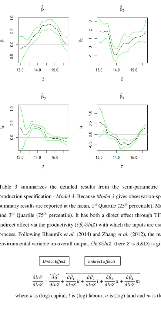
Figure 1 shows the distributions of the semiparametric coefficients across the levels of the R&D variables with 95% confidence intervals. The results show a large variation in the marginal impacts of environmental variable R&D on farm performance in the semi-parametric smooth coefficient model. This heterogeneity in impact is not unexpected because there are many internal and external factors of farms which affects farms’ R&D absorptive capacities. Internal factors of agricultural farms include, “management practices of farms, length of experiences in farming … and the quality of the physical resources of the business including the extent of land degradation and water management. External factors are climate, prices obtained for produce and costs including the cost of financing borrowing (Kilpatrick, 1997 P: 14). In addition, the traditional Cobb-Douglas production model capturing the average (or mean) impact of the R&D variable is not appropriate. The marginal effects of R&D on the elasticities of the factor inputs at the mean and at each of the three quartile values suggest that impact of R&D on production technology is not input neutral. The environmental variable, R&D, affects the marginal productivity of inputs in a non-neutral manner, as indicated in Table 3.
Table 3 summarizes the detailed results from the semi-parametric smooth coefficient production specification - Model 3. Because Model 3 gives observation-specific estimates, the summary results are reported at the mean, 1st Quartile (25th percentile), Median (2nd Quartile), and 3rd Quartile (75th percentile). It has both a direct effect through TFP (∂𝛼̂/∂ln𝑍) and an indirect effect via the productivity (∂𝛽̂𝑖/∂ln𝑍) with which the inputs are used in the production process. Following Bhaumik et al. (2014) and Zhang et al. (2012), the marginal effect of the environmental variable on overall output, ∂lnY⁄∂ln𝑍, (here 𝑍 is R&D) is given by
𝜕𝑙𝑛𝑌 𝜕𝑙𝑛𝑍= 𝜕𝛼̂ 𝜕𝑙𝑛𝑍 ⏞ + 𝜕𝛽̂1 𝜕𝑙𝑛𝑍𝑘 + 𝜕𝛽̂2 𝜕𝑙𝑛𝑍𝑙 + 𝜕𝛽̂3 𝜕𝑙𝑛𝑍𝑎 + 𝜕𝛽̂4 𝜕𝑙𝑛𝑍𝑚 ⏞ (14)
where 𝑘 is (log) capital, 𝑙 is (log) labour, 𝑎 is (log) land and 𝑚 is (log) materials.
The seventh column of Table 3 reports the marginal productivity of R&D (i.e., the elasticity,
∂lnY⁄∂ln𝑍). R&D has a positive effect on output with a mean value of 0.0653, which means that for a 1 per cent increase in R&D investment, the output responds positively by 0.0653 per cent, on average. Though this result is not statistically significant, it seems to be consistent with other study in Australian broadacre agriculture, for example Salim and Islam (2010) found an estimated long-run elasticity of TFP of 0.497 with respect to R&D expenditure. However, their study focuses only for on Western Australian broadacre agriculture where productivity performance is relatively better compared with other states (Khan et al. 2014). Similarly, using national data, Khan et al. (2017) found the long-run elasticities of TFP with respect to R&D lag to be 0.128 in Australian agriculture. This result is also comparable to Zhang et al. (2012) who found the mean R&D elasticity to be 0.1531 in the Chinese high technology industry.
The results also show that there is some variation in the marginal effects of R&D on overall productivity, with a range of effects from -0.11 per cent to 0.52 per cent. These marginal effects are the combined effect of both direct and indirect effects of R&D on productivity. The results reported in column 8 show substantial heterogeneity in the direct effects of R&D on TFP (∂𝛼̂/∂ln𝑍). This article follows the residual based wild bootstrap method to estimate standard errors in the semi-parametric smooth coefficient model.4
4 Following steps are followed: (i) Obtain fitted residuals, ε̂i, from the sample; (ii) Generate wild bootstrap disturbance, εi∗, such that the distribution of two points is as follows: εi∗= aε̂i with probability r = (√5 +
1)/(2√5) and εi∗= bε̂
i with probability 1 − r, where a = −(√5 − 1)/2 and b = (√5 + 1)/2, as
suggested by Hardle and Mammen (1993); (iii) Resample the response variable yi∗ based on the
bootstrapped disturbance, εi∗; (iv) Refit the model using the fictitious response variables; and (v) Repeat
Table 3: Summary of the results for semi-parametric smooth coefficients 1 2 3 4 5 6 7 8 9 10 11 12 Variable 𝛼̂ 𝛽̂1 𝛽̂2 𝛽̂3 𝛽̂4 ∂lnY⁄∂ln𝑍 ∂𝛼̂/∂ln𝑍 ∂𝛽̂1/∂ln𝑍 ∂𝛽̂2⁄∂ln𝑍 ∂𝛽̂3⁄∂ln𝑍 ∂𝛽̂4⁄∂ln𝑍 Mean 3.406 0.3136 0.8299 0.0988 0.0083 0.0653 5.264 0.0136 0.0807 -0.1995 0.1555 (0.5530) (0.1144) (0.1477) (0.0884) (0.1267) (0.0386) (1.2619) (0.0796) (0.2752) (0.1123) (0.0867) 1st Qu. 2.088 0.0357 0.4866 -0.052 -0.262 0.0435 -1.281 -0.4573 -0.7503 -1.1110 -0.4238 (0.0528) (0.0291) (0.0921) (0.0382) (0.0436) (0.0135) (0.9957) (0.0305) (0.1395) (0.1030) (0.0721) Median 3.351 0.3566 1.1284 0.0802 -0.110 0.0521 4.543 0.1913 0.3342 -0.2201 -0.1123 (0.2654) (0.0613) (0.1806) (0.0277) (0.0621) (0.0081) (0.9014) (0.1330) (0.2270) (0.0306) (0.2020) 3rd Qu. 3.809 0.5925 1.5343 0.2994 0.2822 0.0728 11.440 0.4328 1.1600 -0.0664 0.6140 (1.2196) (0.0819) (0.2573) (0.0177) (0.0432) (0.0115) (1.1288) (0.0829) (0.3990) (0.1965) (0.0386) Bootstrapped standard errors in parentheses
The marginal effects of R&D on the factor productivity of inputs vary across the inputs as well as over the observations in the sample. On average, the effects of R&D on input productivity are 0.0136 per cent, 0.0807 per cent, -0.1995 per cent and 0.1555 per cent for capital, labour,
land and materials, respectively. These results indicate that all inputs except land have positive contributions of R&D to productivity, and the effect is biased towards the increased productivity of materials. The greatest variation is found in the marginal effect of R&D on the contribution of labour to output (∂𝛽̂2⁄∂ln𝑍), with minimum and maximum values of -6.63 per cent and 3.43 per cent, respectively. These inputs biased effects of R&D suggest that sectoral reallocation of public R&D investments also matters for the productivity improvement in Australian agriculture. This finding is consistent with other study by Sheng, Jackson and Gooday (2015) that show policy reforms through resource reallocation among farms contribute to the industry-level productivity growth in Australian broadacre agriculture.
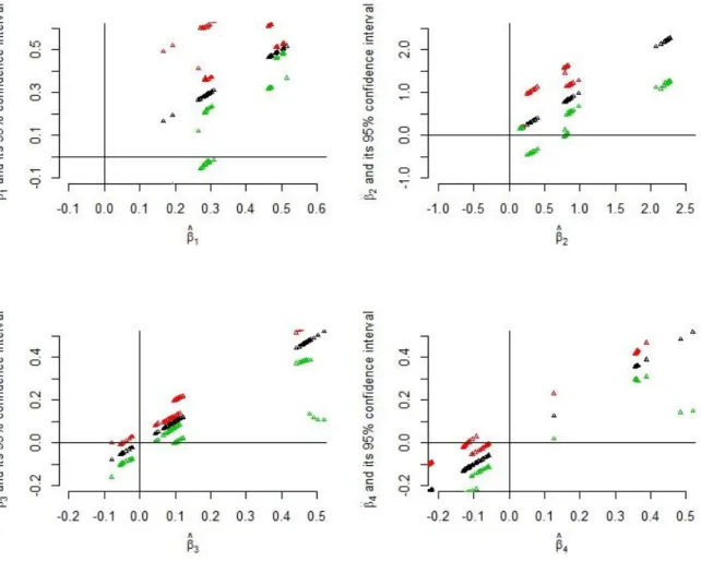
Figure 2 plots the partial effects for each observation in the sample ordered by the value of the estimated coefficient, along with bootstrapped confidence bounds for each of the partial effects. The advantage of this type of plot is that it shows statistical significance for the partial effect of each observation.5 Here the plot shows substantial heterogeneity in the coefficients of the observation-specific partial effects of capital (𝛽̂1), labour (𝛽̂2), land (𝛽̂3) and R&D (∂lnY⁄∂ln𝑍). For most of the observations the lower bounds of the input coefficients, 𝛽̂1, 𝛽̂2, and 𝛽̂3, are greater than zero, indicating positive and statistically significant estimates of output elasticities with respect to capital, labour and land. Turning to the marginal effects of R&D, ∂lnY⁄∂ln𝑍 (where Z is R&D), Figure 2 also shows a plot of the marginal effects of the R&D. It is found that although R&D has both positive and negative effects on output, the effect at the mean is positive and statistically significant. Therefore, only considering the impact of R&D on the average can be misleading when there is non-neutrality in the effects of R&D investment. These statistical results suggest that the R&D variable does not enter the model in the linearly and additively separate fashion that assumed in the conventional parametric specification but the semi-parametric smooth coefficient model has the ability to capture both direct and indirect effects of the environmental variable, R&D. These statistical results are therefore economically meaningful and make the semi-parametric smooth coefficient model
5 The following procedure is followed to construct these plots (Henderson et al. 2012). For any given estimate, say, 𝛽̂1, 𝛽̂1 is plotted against 𝛽̂1, which plots 𝛽̂1 along the 45 degree line. Then, to obtain the
confidence bounds the standard error is added (subtracted) twice from 𝛽̂1, which gives the upper (lower) confidence bounds. The upper and lower confidence bounds are plotted against 𝛽̂1.
more appealing than the corresponding parametric model or Robinson’s semi-parametric model.
Figure 2: Semi-parametric fits: estimates with confidence intervals
Note: Semiparametric fits with bootstrapped confidence intervals
To check the robustness of the estimates, we treat the dataset as a panel (repeated cross section over periods) and use both the fixed effects and the semi-parametric smooth coefficient model. In the semiparametric model with panel data we have controlled state level fixed effects by including state as an unordered categorical variable in the model. The model is estimated employing the local-linear regression estimator approach and presented in appendix Table A.1. As semiparametric estimates of coefficients are functions, we have reported these estimates at their mean. The fixed effects results show that the input coefficients for both capital and labour are positive and significant and that the R&D coefficient is negative but insignificant. In turn, the partial effect of R&D is positive and significant for the semi-parametric smooth coefficient
model with panel data. Plot of the marginal effects of R&D based on panel data is reported also in appendix Figure A.1. These results suggest the estimates are robust for panel data as well.
Technical Efficiency
This paper also considers technical inefficiency in all parametric and semiparametric specifications. Applying standard stochastic frontier approach, we find that the mean technical efficiency for the standard parametric model without z is 0.897 and for the semiparametric model is 0.970. These results are comparable to Sun and Kumbhakar (2013) who found technical efficiencies to be 0.97 and 0.86 for the semiparametric model and parametric model without z, respectively for the Norwegian forestry data. To get an overall view of the distributions of the technical efficiency, we visualize the variation of the technical efficiency estimates using the histogram for each model shown in Figure 3. The figure shows that the efficiency estimates are rather high and an inclusion of z improves the technical efficiency of the farms in the semiparametric specification. Figure 3 also shows that there exist heterogeneities in efficiency levels across the farms under both parametric and semiparametric models, and most of the state-level average farms are almost fully technically efficient under the parametric model with the R&D variable and semiparametric model.
However, for the standard parametric frontier model the estimates of the parameter 𝛾, which indicates the proportion of the total residual variance that is caused by inefficiency is close to zero and statistically not significantly different from zero. This suggests that the inefficiency term is not much relevant in this model and the SFA results are equal to OLS results of the production function. Similarly, the likelihood ratio test that applied to verify the result does not suggest rejecting the null that parametric production function is with no inefficiency term, i.e. there is no significant technical inefficiency. This higher level of efficiency estimates consistent with other studies in Australian broadacre agriculture, for example Islam et al. (2014) found that efficiency gains play an increasingly important role in influencing productivity in Australian broadacre agriculture. Similarly, Sheng et al. (2015) find that the productivity differences among the farms are more likely due to differences in production technology in Australian broadacre agriculture. These results suggest that to improve productivity enhancement of technological capabilities of farms are important, where R&D is an essential element to promote innovation adoption.
Figure 3: Technical Efficiency - Parametric and Semi-parametric model
Note: We also estimate translog production frontier where the efficiency estimates are rather similar to efficiency estimates based on the Cobb-Douglas stochastic production frontier.
The consistent model specification test by Li and Racine (2010) suggests that the environmental factor z is relevant in the semiparametric smooth coefficient frontier model as the p-value is zero which is less than the 1% level of significance. This specification test generally rejects the parametric specifications in favour of more flexible counterparts - the semi-parametric model, i.e., the production function is of the variable coefficient type and that the impact of R&D on output is non-neutral and input specific. However, one limitation of this consistent model specification test is that it is not clear that if misspecification exists in the parametric model, that the semiparametric models is correctly specified. We employed two general types of specification tests, Ullah (1985), based on differences in residuals and Horowitz and Härdle (1994), based on differences in fitted values (as cited in Henderson and Parmeter 2015, Applied Nonparametric Econometrics, chapter 9) to test the semiparametric model versus a nonparametric alternative. With p-values 0 and 0.0075, respectively both tests give the same conclusions that a nonparametric alternative would be preferable. However, with a limited sample size, the semiparametric model may be less subject to the curse of dimensionality problem than a fully nonparametric model. Besides, we could not try fully flexible nonparametric form as our sample size is not as large as required for estimating a nonparametric model (Li et al., 2002). It is also commonly established in the literature that in
Histogram of data$effCD data$effCD F re q u e n cy 0.80 0.85 0.90 0.95 0 5 10 15 Semiparametric SFA TE F re q u e n cy 0.94 0.95 0.96 0.97 0.98 0 5 10 15
Standard SFA without Z Semiparametric SFA
production process in the dataset (Sun and Kumbhakar 2013; Li and Racine 2010; Zhang et al.
2012; Li et al. 2002).
This result is consistent with studies that apply similar methodologies but perform the tests in the manufacturing sector. For example, Li et al. (2002) use the nonparametric kernel method to estimate the semi-parametric varying coefficient model with China’s non-metal mineral manufacturing industry data. They find that the semi-parametric varying coefficient model is more appropriate than either a parametric linear model or a semi-parametric partially linear model. Similarly, using a provincial-level dataset Zhang et al. (2012) suggest that the semi-parametric model yields outcomes that are more intuitive and have fewer economic violations than the parametric counterpart in China’s high technology industry. Further, using the Norwegian forestry data, Sun and Kumbhakar (2013) shows that environmental factors are relevant in semiparametric model, which is preferred that standard parametric model.
The findings of this empirical study suggest that in agricultural production the output does not only depend on input quantities but also on some other variable like public investment in R&D in agriculture. Result also shows that inclusion of R&D variable improves the efficiency in the model and an ignorance of this variable may lead to omitted-variable bias. Moreover, simply including R&D as an additional explanatory variable in applied production analyses does not appropriately capture its influence on the production process, rather a varying coefficients model more properly capture its influence.
5. Conclusion
The conventional econometric approaches ordinarily produce point estimates of the effect of R&D on the productivity of the average unit of analysis assuming implicitly that environmental variables influence productivity neutrally, through the TFP alone, and the differential effect of R&D on factor inputs is not recognized. As a result, the policy implications for R&D investment turn into a one-size-fits-all sort of strategy. Against this backdrop, this article uses a novel econometric methodology, the semi-parametric smooth coefficient model to analyse the effect of R&D on output in Australian broadacre farming. This approach gives rise to the observation-specific estimates of input coefficients. Using state-level average farm data, estimates are provided of the state-level effect of R&D on productivity and the marginal productivity with which factor inputs are used in the production process.
By specifying intercept and slope coefficients as a function of the environmental variable, R&D, the model gives rise to significant variation in the effects of R&D, which confirms the non-neutrality in the effects of R&D on output. Moreover, the result shows that
R&D also affects productivity through inefficiency. The semi-parametric estimates of the effects of public R&D investments on productivity in broadacre farming are more useful than that of parametric estimates in terms of policy implications. First, the results suggest that Australia may enhance its farming productivity by improving investment in public R&D. Second, the large variations in the state-level average farm effects of R&D on productivity imply that initiation of the same R&D policy in different states can have considerably diverse effects on the productivity of inputs. Furthermore, R&D expenditure is found to have a direct impact on productivity and indirect effects through impacting the marginal productivity of factor inputs such as labour and capital. Importantly, none of these issues come into consideration in the parametric regression specifications of modelling the impact of R&D on productivity. This is the fundamental point of interest of using this novel methodology, which provides evidence that the effect of environmental variables on economic performance needs to be revisited. Specifically, consideration should be given to the variations in the effect of R&D on farms performance through technology parameters and through inefficiency. Such variations need to be taken into account when designing policies for investing public R&D in Australian agriculture.
Although the public sector plays a dominant role in R&D investment in Australian agriculture, one of the limitations of this study is that it could not consider the effect of private R&D due to data unavailability. Another limitation is that the within-state farm-level variations in the effects of R&D are not estimated, as data are available only at the state level average farm. In addition, the possibility of errors of measurement with the state-level public R&D data cannot be ruled out. Finally, due to small sample size with only 65 observations, the power of inferences is concerning. At the same time, because of only 13 years of time span, the constructed R&D knowledge stock variable does not reflect R&D’s lag structure properly. Nevertheless, this research explores the relationship from a novel methodological point of view and broadly confirms the results of previous studies regarding the average impact of R&D on productivity, and it provides the additional insight that R&D affects productivity non-neutrally and differentially across farms.
Appendix
Table A.1: Fixed effects and semi-parametric smooth coefficients: panel data
Variables Fixed Effects Model Semi-parametric smooth
coefficient model Capital 0.346* 0.2889** (0.162) (0.0886) Labour 0.856* 0.8525** (0.323) (0.284) Land 0.0457 0.1433 (0.214) (0.0834) Materials -0.0590 0.1154 (0.176) (0.0844) R&D -0.140 0.1024* (0.182) (0.0507) Constant 7.477** 1.0497 (2.230) (1.5153) RTS 1.18 1.40 Observations 65 65 R-squared 0.590 0.9046
Robust standard errors in parentheses; *** p<0.01, ** p<0.05, * p<0.1
6 The pseudo R-squared is derived as the square of the Pearson product moment correlation coefficient, r. This correlation coefficient is based on the correlation between the predicted values and the actual values in the model, which can range from -1 to 1, and so the square of the correlation then ranges from 0 to 1.
References
ABS (2012) Year Book Australia, cat. no. 1301.0. Australian Bureau of Statistics, Canberra Alvarez A, Amsler C, Orea L, Schmidt P (2006) Interpreting and Testing the Scaling Property
in Models Where Inefficiency Depends on Firm Characteristics. Journal of Productivity Analysis 25 (3): 201-212
Ahmad I, Leelahanon S, Li Q (2005) Efficient Estimation of a Semiparametric Partially Linear Varying Coefficient Model. Annals of Statistics 33(1): 258-283
Alene AD (2010) Productivity Growth and the Effects of R&D in African Agriculture. Agricultural Economics 41(3-4): 223-238
Alston JM, Andersen MA, James JS, Pardey PG (2011) The Economic Returns to US Public Agricultural Research. American Journal of Agricultural Economics 93(5): 1257-1277 Ball E, Schimmelpfennig D, Wang SL (2013) Is U.S. Agricultural Productivity Growth
Slowing? Applied Economic Perspectives and Policy 35(3): 435-450
Bhaumik S, Dimov R, Kumbhakar S, Sun K (2014) More Is Better! What Can Firm-Specific Estimates of the Impact of Institutional Quality on Performance Tell Us? (No. 7886). Institute for the Study of Labor (IZA).
Cai, Z., Das, M., Xiong, H. and Wu, X. 2006. Functional Coefficient Instrumental Variables Models. Journal of Econometrics, 133(1), 207-241.
Cai, Z. and Li, Q. 2008. Nonparametric Estimation of Varying Coefficient Dynamic Panel Data Models. Econometric Theory, 24, 1321-1342.
Coe DT, Helpman E (1995) International R&D Spillovers. European Economic Review 39(5): 859-887
Fuglie KO, Toole, AA (2014) The Evolving Institutional Structure of Public and Private Agricultural Research. American Journal of Agricultural Economics. doi: 10.1093/ajae/aat107
Gray EM, Oss-Emer M, Sheng Y (2014) Australian agricultural productivity growth - Past reforms and future opportunities. ABARES research report 14.2, Canberra, February Griffith R, Redding S, Van Reenen J (2004) Mapping the Two Faces of R&D: Productivity
Growth in a Panel of OECD Industries. Review of Economics and Statistics 86(4): 883-895
Griliches Z (1964) Research Expenditures, Education, and the Aggregate Agricultural Production Function. American Economic Review 54(6): 961-974
--- (1979) Issues in Assessing the Contribution of Research and Development to Productivity Growth. Bell Journal of Economics10(1): 92-116
--- (1998) Introduction to "R&D and Productivity: The Econometric Evidence". In R&D and Productivity: The Econometric Evidence. University of Chicago Press: 1-14 Härdle W, Mammen E (1993) Comparing Nonparametric versus Parametric Regression Fits.
Annals of Statistics 21(4): 1926-1947
Hartarska V, Parmeter CF, Nadolnyak D (2011) Economies of Scope of Lending and Mobilizing Deposits in Microfinance Institutions: A Semiparametric Analysis. American Journal of Agricultural Economics 93(2): 389-398
Hastie T, Tibshirani R (1993) Varying-coefficient Models. Journal of the Royal Statistical Society. Series B (Methodological) 55(4): 757-796
Henderson D J, Kumbhakar SC, Parmeter C F (2012) A Simple Method to Visualize Results in Nonlinear Regression Models. Economics Letters 117(3): 578-581.
Henderson DJ, Parmeter CF (2015) Applied nonparametric econometrics. Cambridge University Press
Huffman, W. E., and R. E. Evenson (2006) Do Formula or Competitive Grant Funds Have Greater Impacts on State Agricultural Productivity? American Journal of Agricultural Economics 88(4): 783–798.
Islam N, Xayavong V, Kingwell R (2014) Broadacre Farm Productivity and Profitability in South-Western Australia. Australian Journal of Agricultural and Resource Economics 58(2): 147–170
Kalirajan KP, Obwona M B (1995) Estimating Indivudual Response Coefficients in Varying Coefficients Regression Models. Journal of Applied Statistics22(4): 477–484
Khan F, Salim R, Bloch H (2014) Nonparametric Estimates of Productivity and Efficiency Change in Australian Broadacre Agriculture. Australian Journal of Agricultural and Resource Economics 59(3): 393-411
Khan F, Salim R, Bloch H, Islam N (2017) The Public R&D and Productivity Growth in Australia’s Broadacre Agriculture: Is there a link? Australian Journal of Agricultural and Resource Economics, 61: 285-303.
Kilpatrick, S. (1997). Education and training: Impacts on profitability in agriculture, Australian and New Zealand Journal of Vocational Education Research 5: 1–36.
Li Q, Huang CJ, Li D, Fu TT (2002) Semiparametric Smooth Coefficient Models. Journal of Business & Economic Statistics 20(3): 412-422
Li Q, Racine JS (2007) Nonparametric Econometrics: Theory and Practice. Princeton University Press: 301-312
--- (2010) Smooth Varying-Coefficient Estimation and Inference for Qualitative and Quantitative Data. Econometric Theory 26(6): 1607-1637
Mamuneas TP, Savvides A, Stengos T (2006) Economic Development and the Return to Human Capital: A Smooth Coefficient Semiparametric Approach. Journal of Applied Econometrics 21(1): 111-132
Manski CF (2003) Partial identification of probability distributions. New York: Spring-Verlag Mullen J (2007) Productivity Growth and the Returns from Public Investment in R&D in Australian Broadacre Agriculture. The Australian Journal of Agricultural and Resource Economics51(4): 359-384
--- (2010) Trends in Investment in Agricultural R&D in Australia and its Potential Contribution to Productivity. Australasian Agribusiness Review 18(2): 18-29
Mullen JD, Scobie GM, Crean J (2008) Agricultural Research: Implications for Productivity in New Zealand and Australia. New Zealand Economic Papers 42(2): 191-211
Nossal K, Sheng Y (2010) Productivity growth: Trends, drivers and opportunities for broadacre and dairy industries. Australian commodities: Forecasts and Issues 17(1): 216-230