Sensitivity to model misspecification of the Von Bertanlanffy grown model with measurement error in age

(1)

Sensitivity to Model Misspecification of the Von

Bertanlanffy Growth Model with Measurement

Error in Age

by

c

Rajib Dey

A thesis submitted to the School of Gradate Stud-ies in partial fulfillment of the requirements for the degree of Master of Science.

Department of Mathematics and Statistics

Memorial University

September 2017

(2)

Abstract

The Von Bertalanffy growth function (VonB) specifies the length of a fish as a function of its age. However, in practice, age is measured with error. We study the structural errors-in-variables (SEV) approach to account for measurement error (ME) in age. Cope and Punt (2007) also proposed this approach for fish growth data. They as-sumed unobserved age had a simple Gamma distribution. In this study, we investigate whether SEV VonB parameter estimators are robust to the Gamma approximation of true unobserved ages. By robust we mean lack of bias due to ME and model mis-specification. Our results demonstrate that this method is not robust. We propose a flexible parametric Normal mixture distribution for the unobserved true ages to reduce this bias when estimating the length-age relationship with a VonB model. We investigate the performance of this approach in comparison to the Gamma age model through extensive simulation studies and a real-life data set.

(3)

(4)

Acknowledgements

I would like to express my most sincere and deepest gratitude to my supervisor, Dr. Noel Cadigan. This thesis would not have been completed without his excellent guid-ance, generous support and continuous motivation. I would also like to thank him for his exceptional generosity with his time and energy in my PhD application.

I offer my very special thanks to Dr. Taraneh Abarin, my co-supervisor, for her suggestions and guidance throughout this study. I am very grateful for the hospitality I was offered during many holiday parties over the last two years.

I gratefully acknowledge the funding received towards my MSc from School of Graduate Studies, the Department of Mathematics and Statistics, and my supervisor in the form of graduate fellowships and teaching assistantships.

My sincere thanks go to all the professors from the Statistics wing, MUN for all their help and support. I am grateful to Dr. JC Loredo-Osti and Dr. Zhaozhi Fan, for giving me suggestions and help in my PhD application.

Furthermore, I would like to thank Center for Fisheries Ecosystems Research, Fish-eries and Marine Institute of MUN for creating a friendly and comfortable working

(5)

environment. Thanks to Karen Dwyer at the Department of Fisheries and Oceans in St. John’s, NL, for providing the data used in this thesis and for helpful discussions about my research.

Last but most importantly, I am very grateful to my parents and my younger sister for their strong belief in my capabilities and for all of their eternal love, support and encouragement during my stay far away from them.

(6)

List of tables

2.1 Estimated values of L∞, k, and ao based on the SEV VonB Gamma model, versus the proportion of old aged fish in the population (Pr) and skewness of the distribution. . . 47 2.2 SEV VonB estimates of L∞, k, andao, versus skewness of the

distribu-tion at Pr = 0.001. . . 47 2.3 SEV VonB estimates of L∞, k, andao, versus skewness of the

distribu-tion at Pr = 0.04. . . 47

3.1 Sensitivity to model misspecification: The true unobserved age distri-bution is a mixture of three Gamma distridistri-butions, which is misspecified as the two-Normal mixture (G = 2) and the three-Normal mixture (G = 3) distributions. Results for estimated values, and standard error(SE) for L∞, k and ao. . . 66

3.2 Sensitivity to model misspecification: The true unobserved age dis-tribution is a Lognormal with µ = 1.275 and σ = 0.4723, which is misspecified as the two-Normal mixture and the Gamma distributions. Results for absolute bias(abias), percentage error(PE), and standard error(SE) for L∞, k and ao. . . 67

(12)

3.3 Sensitivity to model misspecification: The true unobserved age distri-bution is a mixture of three Gamma distridistri-butions, which is misspecified as the two-Normal mixture and the Gamma distributions. Results for absolute bias(abias), percentage error(PE), and standard error(SE) for

L∞, k and ao. . . 68

3.4 Sensitivity to model misspecification: The true unobserved age distri-bution is a mixture of three truncated Normal distridistri-butions, which is misspecified as the two-Normal mixture and the Gamma distributions. Results for absolute bias(abias), percentage error(PE), and standard error(SE) for L∞, k and ao. . . 69

3.5 Sensitivity to model misspecification: The true unobserved age distri-bution is a mixture of ten Gamma distridistri-butions, which is misspecified as the two-Normal mixture and Gamma distributions. Results for ab-solute bias(abias), percentage error(PE), and standard error(SE) for

L∞, k and ao. . . 70 3.6 Comparison of the two-mixture Normal age distributions with the true

age Lognormal distribution. Results for absolute bias(abias), percent-age error(PE), and standard error(SE) for L∞, k and ao. . . 71

5.1 Summary table of length and age of Greenland Halibut. The results for mean, median and coefficient of variation (CV) for length and age of Greenland Halibut by their sex. . . 98 5.2 Parameter estimation results of Greenland Halibut based on the SEV

VonB G-Normal mixture BI model for different assumed values of ME in age (σ_ua). The results for the estimated values and its corresponding standard errors (SE) of the parameters based on the full data. . . 98

(13)

5.3 Parameter estimation results of Greenland Halibut female fish based on the SEV VonB G-Normal mixture BI model for different assumed values of ME in age (σa_u). The results for the estimated values and its corresponding standard errors (SE) of the parameters based on the female data. . . 99 5.4 Parameter estimation results of Greenland Halibut male fish based on

the SEV VonB G-Normal mixture BI model for different assumed val-ues of ME in age (σ_ua). The results for the estimated values and its corresponding standard errors (SE) of the parameters based on the male data. . . 99

C.1 Sensitivity to model misspecification: The true unobserved age distri-bution is Lognormal withµ= 1.275 andσ = 0.4723,which is misspeci-fied as the two-Normal mixture and the Gamma distributions. Results for average estimated values, and root mean squared errors(RMSE) of

L∞, k, ao and σc were based on repeated Sampling. . . 117 C.2 Sensitivity to model misspecification: The true unobserved age

distri-bution is a mixture of three Gamma distridistri-butions, which is misspeci-fied as the two-Normal mixture and the Gamma distributions. Results for average estimated values, and root mean squared errors(RMSE) of

(14)

List of figures

1.1 Simulation-Extrapolation (SIMEX) estimate ˆβ1(λ) of slope parameter

of simple linear model. The simulated measurement error denoted by λ. 22 1.2 Application of the Von Bertalanffy (VonB) model for L∞ = 120, k =

0.2. The top panel illustrates the growth curve when a0 = 0, and the

bottom panel illustrates when a0 < 0. YT and XT denote the true length and true age of fish, respectively. . . 23 1.3 Average simulated values of Von Bertalanffy (VonB) parametersL∞, k

& ao estimated using the nonlinear least squares method. The mea-surement error variance is denoted by σu. . . 24 2.1 Sensitivity analysis of large sample bias in the estimates of β0 and β1

based on the SEV linear model where two true covariate Normal

distri-butions, i.e., Normal(1.5,1) and Normal(0.5,1) misspecified as Normal(µ, µ2). 42 2.2 True unobserved age (XT) distribution is Lognormal with mean,E(XT)

(15)

2.3 Sensitivity analysis of large sample bias in the estimates of L∞, k, and

ao based on the SEV VonB Gamma model. Results were based on simulating data from a correctly specified Gamma distribution and six misspecified Lognormal distributions with different means, E(XT) and skewness, Sk. . . 44 2.4 True unobserved age (XT) mixture Gamma and truncated Normal

dis-tributions. . . 45 2.5 Sensitivity analysis of large sample bias in the estimates of L∞, k, and

ao based on the SEV VonB Gamma model. Results were based on sim-ulating data from a correctly specified Gamma distribution and three misspecified mixture distributions. . . 46

4.1 Sensitivity analysis of bias in the average estimates of L∞, k, ao and σc based on the SEV VonB BI model. The true unobserved age distribu-tion is a Lognormal distribudistribu-tion with µ= 1.275 and σ = 0.4723 which is misspecified as the two-Normal mixture and Gamma distributions. . 85 4.2 Sensitivity analysis of root mean squared error (RMSE) in the average

estimates of L∞, k, ao and σc based on the SEV VonB BI model. The true unobserved age distribution is a Lognormal distribution with µ= 1.275 and σ= 0.4723 which is misspecified as the two-Normal mixture and Gamma distributions. . . 86 4.3 Sensitivity analysis of bias in the average estimates of L∞, k, ao and σc

based on the SEV VonB BI model. The true unobserved age distribu-tion is a mixture of three Gamma distribudistribu-tions which is misspecified as the two-Normal mixture and Gamma age distributions. . . 87

(16)

4.4 Sensitivity analysis of root mean squared error (RMSE) in the average estimates of L∞, k, ao and σc based on the SEV VonB BI model. The true unobserved age distribution is a mixture of three Gamma distri-butions which is misspecified as the two-Normal mixture and Gamma age distributions. . . 88 4.5 The estimated values based on the SEV VonB G-Normal mixture BI

model estimators ofL∞, k, ao andσc,when the true measurement error variance in age (σu = 0.05) is wrongly assumed by σau. The true unob-served age distribution is a Lognormal with µ= 1.275 andσ = 0.4723,

which is misspecified as the two-Normal mixture distribution. The first and third quartiles of the estimated parameters are presented. . . 89 4.6 The estimated values based on the SEV VonB G-Normal mixture BI

model estimators ofL∞, k, ao andσc,when the true measurement error variance in age (σu = 0.15) is wrongly assumed by σau. The true unob-served age distribution is a Lognormal with µ= 1.275 andσ = 0.4723,

which is misspecified as the two-Normal mixture distribution. The first and third quartiles of the estimated parameters are presented. . . 90

5.1 Length versus age plot of the Greenland Hailbut fish by their sex. The data collected by NAFO management unit Subarea 2 + Divisions 3kLMNO. . . 97

C.1 Frequency distribution of ˆL∞(σu),kˆ(σu), ˆao(σu) & ˆσc(σu) based on the SEV VonB two-Normal mixture BI model. The true unobserved age distribution is a Lognormal with µ = 1.275 and σ = 0.4723 which is misspecified as the two-Normal mixture distribution. We consider the sample size 200. . . 119

(17)

C.2 Frequency distribution of ˆL∞(σu),kˆ(σu), ˆao(σu) & ˆσc(σu) based on the

SEV VonB Gamma BI model. The true unobserved age distribution is a Lognormal with µ = 1.275 and σ = 0.4723 which is misspecified as the Gamma distribution. We consider the sample size 200. . . 119 C.3 Frequency distribution of the estimates ˆL∞(σu),kˆ(σu), ˆao(σu) & ˆσc(σu)

based on the SEV VonB two-Normal mixture BI model. The true unobserved age distribution is a Lognormal with µ = 1.275 and σ = 0.4723 which is misspecified as the two-Normal mixture distribution. We consider the sample size 400. . . 120 C.4 Frequency distribution of the estimates ˆL∞(σu),kˆ(σu), ˆao(σu) & ˆσc(σu)

based on the SEV VonB Gamma BI model. The true unobserved age distribution is a Lognormal with µ = 1.275 and σ = 0.4723 which is misspecified as the Gamma distribution. We consider the sample size 400. . . 120 C.5 Frequency distribution of the estimates ˆL∞(σu),kˆ(σu), ˆao(σu) & ˆσc(σu)

based on the SEV VonB two-Normal mixture BI model. The true un-observed age distribution is a mixture of three Gamma distributions which is misspecified as the two-Normal mixture distribution. We con-sider the sample size 200. . . 121 C.6 Frequency distribution of the estimates ˆL∞(σu),kˆ(σu), ˆao(σu) & ˆσc(σu)

based on the SEV VonB Gamma BI model. The true unobserved age distribution is a mixture of three Gamma distributions which is mis-specified as the Gamma distribution. We consider the sample size 200. 121

(18)

C.7 Frequency distribution of the estimates ˆL∞(σu),kˆ(σu), ˆao(σu) & ˆσc(σu) based on the SEV VonB two-Normal mixture BI model. The true un-observed age distribution is a mixture of three Gamma distributions which is misspecified as the two-Normal mixture distribution. We con-sider the sample size 400. . . 122 C.8 Frequency distribution of the estimates ˆL∞(σu),kˆ(σu), ˆao(σu) & ˆσc(σu)

based on the SEV VonB Gamma BI model. The true unobserved age distribution is a mixture of three Gamma distributions which is mis-specified as the Gamma distribution. We consider the sample size 400. 122

(19)

Chapter 1 Introduction

1.1 Measurement Error

The purpose of regression analysis is to make inference about a mathematical model expressed in terms of an explanatory variable X. However, due to different reasons, the most obvious being the inaccuracy of measurements, X may not be observable. Hence, we considerXT to be the true but unobservable covariate and instead of it we observeX as a proxy variable. The substitution of X for XT complicates statistical analysis and creates problems due to the error in the measurement ofXforXT. Error in covariates is a problem in many scientific areas. For example, in fisheries science, error in age estimates for individual fish could be a consequence of misinterpretation by readers of ageing structures (e.g. scales and otoliths) or inability of ageing structures to accurately record growth sequence information.

Special estimation methods are needed when a covariate in a model is measured with error. Regression analysis ignoring this error is known to produce biased and falsely precise estimates of the regression parameters (e.g. Fuller, 2009 [21]; Carroll et al., 2006 [12]). Further effects are unreliable coverage levels of confidence intervals

(20)

1.1. MEASUREMENT ERROR 2

and reduced power of hypothesis tests.

1.1.1 Measurement Error Models

Specification of a model for the measurement error (ME) process is necessary for analyzing a ME problem. There are two general approaches:

Classical ME Model: This is appropriate when a quantity is measured by some device and repeated measurements vary around the true value. The model can be specified as

X =XT +U,

whereU, the ME, is assumed to be independent of XT with mean zero and variance

σ2

u,which is the ME variance.

Berkson Error Model: This is appropriate in a situation when a group’s average is assigned to each individual suiting the group’s characteristics. The group’s average is thus the measured value; i.e., the value that enters the analysis, and the individual value is the true value. This type of error model can be defined as

XT =X+U,

whereU is assumed to be independent of X with mean zero and varianceσ_u2.

Finally, a very important difference between classical ME and Berkson error models is that in the classical model, the variability of the observed X is larger than the variability of the true XT. In the Berkson model it is the other way around. One needs information about the data structure in order to perform a ME analysis.

(21)

1.1.2 Sources of Data

The data sources can be separated into two main categories, 1) internal subsets of the primary data, and 2) data from external or independent sources. Within each of these broad categories, there are three types of data described in Carroll et al. (2006) [12] which are as follows:

1. Validation Data: In which XT is observed directly. 2. Replication Data: In which replicates of X are available.

3. Instrumental Data: If the ME is unknown then one needs to estimate it with the validation data or replicate measurements of X. However, it is not always possible to obtain replicates, and thus estimation of ME varianceσuis sometimes impossible. When there is no information about the σu, the estimation of re-gression parameters is still possible if the data contains an instrumental variable

I in addition toX. I must be observed and correlated with XT. Furthermore, it must be uncorrelated with the ME, U =X₋XT.

1.1.3 Differential and Non-differential Errors

It is important to make a distinction between differential and non-differential MEs. Non-differential ME occurs in a broad sense when one would not be concerned with

X if XT were available. This is the type of error in a fish growth model, e.g. when the true age (XT) of a fish is known then the observed age (X) measured with error does not have any information about the length of fish (Y). Let the conditional pdf ofY givenXT =xT be fY|XT(y|xT),and the conditional pdf ofX givenXT =xT be

(22)

When ME is non-differential then the joint pdf of (Y,X) given XT =xT is

fY,X|XT(y, x|xT) =fY|XT(y|xT)fX|XT(x|xT). (1.1) However, when ME is differential, using standard conditioning arguments, the joint pdf of (Y,X) givenXT =xT becomes

fY,X|XT(y, x|xT) =fY|XT(y|xT)fX|Y,XT(x|y, xT). (1.2) Note that the only difference between Eqns. (1.1) and (1.2) is in the ME term. In the former, under non-differential ME,X and Y are independent whenXT is given. Therefore, one can estimate parameters in models for responses even when the true covariates are not observable. However, parameter estimation is difficult when ME is differential, since we must determine the conditional distribution of X given XT and the response Y. This is essentially impossible to do in practice unless one has a subset of the data in which all of (Y;X;XT) are observed, i.e., a validation data set.

1.1.4 Model Identification

Model identification is an important aspect of ME modeling. A model is identified if all its parameters can be uniquely estimated from the data. According to Fuller (2009) [21], the parameter θ of the distribution of a random variable Z, with distribution function FZ(z;θ), is identified if, for any two parameters in the parameter space,

θ1 6=θ2, (θ1, θ2)∈Θ,FZ(z;θ1)6=FZ(z;θ2) for at least one value ofz. If the parameters

(23)

1.1.5 The Effect of ME in Simple Linear Regression

The linear model specifies Y as a function ofXT,

Y =βo+β1XT +ǫ, (1.3)

whereβ0 and β1 are the intercept and slope parameters, respectively. Suppose XT is measured with the classical ME model and defined as

X =XT +U. (1.4)

Assume thatǫand U followN(0, σ2

e) andN(0, σu2), respectively. Further, assume that

XT follows aN(µxT, σ

2

xT) and that XT, ǫ and U are mutually independent. Then the multivariate Normal distribution (MVN) of (XT, U, ǫ) is

      XT U ǫ       ∼M V N             µxT 0 0       ,       σ_x2_T 0 0 0 σ2_u 0 0 0 σ2_e             . (1.5)

Therefore, the bivariate Normal distribution (BVN) of (ǫ, XT) is    ǫ XT   =    Y ₋(βo+β1XT) X₋U   ∼BVN       0 µxT   ,    σ_e2 0 0 σ2 xT      . (1.6) By rearranging Eqn. (1.6), the BVN of (Y, X) is

   Y X   ∼BVN       µ1 µ2   ,    σ11 σ12 σ21 σ22      , (1.7)

(24)

whereµ1 =E(Y) = βo+β1µxT,µ2 =E(X) = µxT, and the elements of the variance-covariance matrix of the BVN of (Y, X) are

σ11 = V(βo+β1XT +ǫ) =β12σx2T +σ 2 e, σ22 = V(X) = V(XT +U) =σx2T +σ 2 u,

σ12 = Cov(Y, X) = Cov(βo+β1XT +ǫ, XT +U) = Cov(β1XT, XT) =β1σx2T. Finally, the BVN in Eqn. (1.7) is

   Y X   ∼BVN       β0+β1µxT µxT   ,    β2 1σx2T +σ 2 e β1σx2T β1σx2T σ 2 xT +σ 2 u      . (1.8) Attenuation Bias: If the true covariate XT were observed in a sample of size n observations (Yi, XTi) of (Y, XT), the ordinary least squares (OLS) estimator of β1 of the linear model in Eqn. (1.3) is

ˆ β₁∗ = Pn i=1(XTi−X¯T)(Yi−Y¯) Pn i=1(XTi−X¯T)2 . (1.9)

In the presence of ME, the model involving the measured value ofXT,X, is

Y =β0+β1X+ǫ∗, (1.10)

where ǫ∗ ₌ ₋_β

1U +ǫ. Given a random sample of n observations (Yi, Xi) of (Y, X), the OLS estimator ofβ1 for the model in Eqn. (1.10) is

ˆ β1 = Pn i=1(Xi−X¯)(Yi−Y¯) Pn i=1(Xi−X¯)2 . (1.11)

(25)

According to Fuller (2009) [21] if (Y, X) is a bivariate Normal vector (Eqn. 1.8), then the expected value of ˆβ1 is given by

E[ ˆβ1] = Cov(X, Y) V(X) = Cov(XT +U, Y) V(XT +U) = Cov(XT +U, β0+β1XT +ǫ) V(XT) + V(U) =β1 σ2_x_T σ2 xT +σ 2 u =β1(1− σ_u2 σ2 xT +σ 2 u ). (1.12)

In addition, X and ǫ∗ are correlated with each other, i.e.,

Cov[X, ǫ∗] = Cov[XT +U, ǫ−β1U] =−β1σ2u 6= 0.

Hence, from Eqn. (1.12), E[ ˆβ1]6=β1; consequently, the OLS estimator of β1 is biased

and inconsistent. The expected value of ˆβ1 is attenuated toward zero when the ME

is large. The bias does not reduce with increasing sample size, n. The extent of the attenuation is measured by the quantity Λ = σxT2

σ2

xT+σ2u, which is known as the reliability ratio.

Model Identification: Model identification is a key issue here. All the parameters in the model can be represented by the vector, θ = (β0, β1, µxT, σ

2

xT, σ

2

u, σe2). The BVN distribution in Eqn. (1.8) is completely determined by its mean and variance-covariance matrix, which involve E(Y),E(X),V(X),V(Y), and Cov(X, Y). Each of these are functions of the six elements ofθ. Hence, there are many parameter vectorsθ

that produce the same mean vector and variance-covariance matrix of the BVN. Thus by definition, the model defined in Eqns. (1.3)-(1.4) is not identified. This ME model

(26)

is identified if one of the parameter values is known in addition to the information in the sample. For example, if σ2_u is known then the other values of the parameters uniquely determine the BVN distribution of X and Y.

The OLS of β1 can be corrected for bias to get the best linear unbiased estimator

of β1. This can be achieved when the reliability ratio Λ is known. By rearranging

Eqn. (1.12), a bias-corrected estimator of β1 is

E[ ˆβ1Λ−1] =β1. (1.13)

1.1.6 ME Methods

In the previous section, we showed that the OLS estimator is typically biased when there is covariate ME, and the direction as well as severity of the bias increases with the magnitude of the ME.

Two basic methods have been used in ME models (e.g. Stefanski, 2000 [43]). We review the functional and structural based methods in the following sections.

Functional Errors-in-Variables

In functional errors-in-variables (FEV) models, the unobserved true covariates are modeled as unknown, nonrandom constants (i.e. parameters) (e.g. Carroll et al., 2006 [12]). In this model, with a sample of sizen, we have n measurements of unobserved true covariates; hence, the parameter vector includesXT1, XT2, ...., XTn and the num-ber of parameters increases linearly withn. When the number of nuisance parameters is large relative to n it is well known that maximum likelihood estimators (MLEs) for some parameters, particularly for variance parameters, can be largely biased and inconsistent (e.g. section 4.3 in Barndorff and Cox, 1994 [3]; Berger et al., 1999 [4]).

(27)

Finding a conditional distribution or score function that does not depend on nui-sance parameters is one approach to deal with this bias problem due to many nuinui-sance parameters. Methods based on FEV models can be divided into approximately con-sistent (remove most bias) and fully concon-sistent methods (remove all bias asn _{→ ∞}). Fully consistent methods for nonlinear regression models typically require assump-tions on the distribution of the ME. Regression calibration and SIMEX are examples of approximately consistent methods while corrected scores and conditional scores methods are fully consistent for large classes of models.

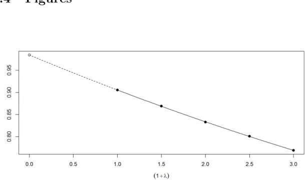
Simulation-Extrapolation (SIMEX): The underlying concept of SIMEX, pro-posed in Cook and Stefanski (1994) [14] and further developed by Stefanski and Cook (1995) [42], is to determine the effect of ME on the parameter estimator experimentally via simulation, assuming that the ME variance is known or estimated from validation data. A detail discussion of the method can be found in Carroll et al. (2006) [12]. The SIMEX algorithm is executed in two steps: Simulation and Extrapolation.

1. Simulation Step: Computer simulated ME (i.e. random error) is added to the observed measurement X and the biased parameter estimate is computed with the additional simulated pseudo error terms. This process is repeated for several increments in the value of the simulated ME.

2. Extrapolation Step: It consists of modeling the trend between the biased parameter estimates and the corresponding size of the simulated ME. A nearly unbiased SIMEX estimator is then obtained by extrapolating the trend back to the point of zero ME.

We explain this concept with the simple linear model. We generated 1000 observations of XT from a standard Normal distribution. Then, we generated 1000 observations

(28)

of Y assuming a linear model (Eqn. 1.3) using the β0 = 0, β1 = 1, σe = 1 and XT. We use σu = 0.3 in the Eqn. (1.4) to generate 1000 observations of X. We have considered the simulated ME λ such as 0.5, 1, 1.5 and 2. We randomly generate b = 100 independent datasets for each λ. For each (say bth_{) dataset we follow the}

following steps:

• Step 1: We generated simulated pseudo errors Zb,i (i = 1, 2,. . . , 1000) from a standard Normal distribution.

• Step 2: We generate pseudo predictors Xb,i(λ) = Xi + λ0.5 σu Zb,i (i = 1, 2,. . . , 1000) for a specific value of λ.

• Step 3: Fit the linear model to (Yi, Xb,i(λ)) for a specific value of λ. We used OLS method to estimate the slope parameter which is ˆβ1,b(λ).

Repeat these steps b times and calculate the average simulation estimate ofβ1, ˆβ1(λ) = 1

b Pb

i=1βˆ1,i(λ). We plot the ˆβ1(λ) against each value of (1 +λ). We use a quadratic

extrapolation fitting method to the trend back to the point of zero ME, i.e., λ=₋1. Figure 1.1 illustrates that the SIMEX estimate ˆβ1(λ) changes as added simulated ME

increases. To estimate ˆβ1 if there is no ME we use a quadratic extrapolation fitting

method to the trend back to the point of zero ME, i.e.,λ=₋1. The estimated value of β1 is 0.985 while the true value of β1 was 1.

Regression Calibration: Regression Calibration (RC) was introduced by Prentice (1982) [33] in a proportional hazards model application and generalized by Carroll and Stefanski (2006) [10] to increase its scope. The method and its applications are discussed extensively in Carroll et al. (2006) [12]. The RC algorithm is as follows:

• Step 1: Estimate the regression of XT on X using replication or validation data. This is called the calibration function.

(29)

• Step 2: Replace the unobserved XT by its estimate from the regression model, and then run a standard analysis to obtain parameter estimates.

• Step 3: Adjust the resulting standard errors to account for the estimation at the step 1, using either the bootstrap or asymptotic methods.

There are two important drawbacks of RC, 1) for linear and log-linear models RC provides asymptotically unbiased estimators whereas for nonlinear models the RC estimator is approximately unbiased (e.g. Buzas et al., 2003 [7]); 2) standard errors for parameter estimates are obtained from bootstrapping or asymptotic normal assumptions; consequently, statistical inference is not exact.

Structural Errors-in-Variables

In structural errors-in-variables (SEV) models the observed X and true unobserved covariateXT are jointly considered to be random and vary in repeated sampling. Let

Y be the response variable, and we define YT as a function of XT,

YT =g(XT;θR), (1.14) where the mean function g(.) is a continuous real valued function and θR is the pa-rameters of the mean function. We define the classical ME models as

Y =YT +ǫ, (1.15)

(30)

where ǫ follows N(0, σ_e2), and U follows N(0, σ_u2) with σ_u2 is known. We assume that the conditional pdf of Y givenXT =xT is

fY|XT(y|xT;θR), and the conditional pdf of X given XT =xT is

fX|XT(x|xT;σu). The joint pdf of (Y,X) is

fY,X(y, x;θ) = Z Z

fY,X|YT,XT(y, x|yT, xT;θR, σu)fXT,YT(xT, yT;θR, θE) ∂yT ∂xT, whereθ = (θR, θE). We assume that MEs inX and Y are independent so that

fY,X|YT,XT(y, x|yT, xT;θR, σu) =fX|XT(x|xT;σu) fY|YT(y|yT;θR). (1.17) The joint pdf of (YT,XT) can be expressed as

fXT,YT(xT, yT;θR, θE) = fYT|XT(yT |xT;θR) fXT(xT;θE). (1.18) Combining Eqns. (1.17)-(1.18), the joint pdf of (Y,X) is

fY,X(y, x;θ) = Z Z

fX|XT(x|xT;σu)fY|YT(y |yT;θR)fYT|XT(yT |xT;θR)fXT(xT;θE)∂yT ∂xT. If we know the true covariate XT, then we assume that we would know the true

(31)

for a true covariateXT; hence,

fYT|XT(yT |xT;θR) =      1 yT =g(xT;θR) 0 otherwise. (1.19)

Eventually, under the above assumption,

fY|YT(y |yT;θR) = fY|XT(y|xT;θR). Therefore, the joint pdf of (Y,X) is

fY,X(y, x;θ) = Z

fY|XT(y|xT;θR)fX|XT(x|xT;σu) fXT(xT;θE) dxT. (1.20) The integral is replaced by a sum ifXT is a discrete random variable. In Eqn. (1.20), 1. Response Model: fY|XT(y|xT;θR) describes the relationship between Y and

XT;

2. ME Model: fX|XT(x|xT;σu) describes the relationship between X and XT; 3. Covariate Model: The true unobserved covariate XT is considered as a

ran-dom variable with pdf fXT(xT;θE).

The likelihood for the observed data is then maximized over all the parameters in two of the above three component distributions, i.e., response model and covariate model, to obtain MLEs of the parameters.

The SEV approach requires parametric distributional assumptions for the unob-served covariate,XT, which none of the preceding FEV methods required. It is com-mon to assume a Normal distribution for the covariate model, but unless there are validation data, it is not possible to assess the adequacy of the covariate model using

(32)

the data. In SEV models, the distribution ofXT is speculative and could be quite dif-ferent from it’s true underlying distribution leading to model misspecification. Hence, an important concern is whether the SEV estimates are robust to misspecification of the distribution of the true covariate. The sensitivity of the regression parameters estimators to covariate model misspecification in SEV models has been illustrated in Carroll, Roeder and Wasserman (1999) [11].

Semi-parametric and flexible parametric modeling are two approaches that have been explored to address potential robustness issues in specifying a pdf forXT. Semi-parametric methods leave the pdf forXT unspecified, and the pdf forXT is essentially considered as another parameter that needs to be estimated. These models have the advantage of model robustness but may lack efficiency relative to the full likelihood (e.g. Suh and Schafer, 2002 [45]). A flexible parametric model is described in Carroll, Roeder and Wasserman, 1999 [11], where mixtures of Normals were used to approx-imate the covariate model (since the true covariate model is generally unknown) to estimate the parameters of a linear errors-in-variables model and a change-point Berk-son model. Flexible parametric approaches have been studied in, e.g. Kuchenhoff and Carroll (1997) [30], Schafer (2002) [39].

The choice between functional or structural models depends both on the assump-tions one is willing to make and, in a few cases, the form of the model relating Y to X. To explain this point we have taken one of the examples stated in Fuller (2009) [21]. Consider the relationship between yield of corn, say Y, and available nitrogen, say XT, in the soil. To estimate the available soil nitrogen, it is necessary to sample the soil of the experimental plot and to perform a laboratory analysis on the selected sample. As a result of the sampling and of the laboratory analysis, we observe X

(33)

1.2. FISH GROWTH AND ME 15

interpretations of the true values XT. First, assume that the fields are a set of ex-perimental fields managed by the experiment station in ways that produce different levels of soil nitrogen in the different fields. In such a situation, one would treat the true, but unknown, nitrogen levels in the different fields as fixed. In this case the FEV approach is a natural choice. On the other hand, if the fields were a random sample of farmers fields, the XT could be treated as random variables. In this case SEV is preferable. In addition, the type and amount of data available also play role. For example, validation data provides information on the distribution ofXT, and may make structural modeling more preferable.

To sum up, the SEV approach can yield high efficiency and allow construction of likelihood-based inference, whereas this may be more difficult in FEV models due to the large number of parameters. However, robustness in SEV estimates is an impor-tant issue due to misspecification of the covariate model. Despite this shortcoming, SEV models are more common and usually preferable to FEV models because of the general applicability of SEV models, and their simple computation and potential gain in efficiency.

1.2 Fish Growth and ME

Body growth is an important factor in fish population dynamics and determining sustainable levels of fishing. Growth varies from species to species, for different pop-ulations of a species (i.e. stocks), and different year-classes within a population (e.g. Chen and Mello, 1999 [13]). Growth information is essential for fish stock assessment which is a process that produces scientific advice on the health of a fish stock and the impacts of fisheries. Fishing quotas are usually based on weight whereas mortality involves the number of fish in a stock. Good information about body growth rates

(34)

are required to predict the impacts of future fishing quotas on stock mortality and when deciding what are good and sustainable harvest rates. Poor information on body growth rates may lead to incorrect prediction of the mortality impacts of fishing and other population dynamics (e.g. Vincenzi et al., 2014 [49]). Therefore, estimation of growth rates is a common and important part of fisheries stock assessment studies. Generally, two basic types of growth data are available from commercial fisheries: 1) age-to-length data in which one age and length measurement per fish is collected from a large sample of fish, and 2) multiple measurements of the same fish via capture-recapture or other repeated measures studies (e.g. Francis, 1988 [19]). The first type of data is more common. Ages are determined by counting growth bands in ear bones (otoliths) and this can involve substantial error especially for older fish because the bands get harder to differentiate as a fish gets older. There are several growth models available in literature; however, the Von Bertanlanffy growth model is the most widely used and its parameters are useful for describing a fish growth curve as discussed in Von Bertalanffy (1960) [50].

1.2.1 Von Bertanlanffy (VonB) Growth Model

The theory of the VonB model is based on the assumption that the change in length per unit time, dYT

dXT, declines with length. That is, the growth rate of large individuals is less than the growth rate of small individuals. IfYT denotes the length at age XT, then the VonB growth rate model is based on the differential equation

dYT

dXT

=k(L∞−YT), (1.21)

and dYT

dXT = 0 when YT =L∞. Thus, the growth rate of fish will get smaller and even-tually becomes zero as a fish nears its maximum possible length L∞. The parameter

(35)

L∞ is the asymptotic length at which the growth rate is zero andk is the growth rate

parameter. Assuming thatYT = 0 when XT = 0, the solution of Eqn. (1.21) is

YT =L∞(1−e−kXT).

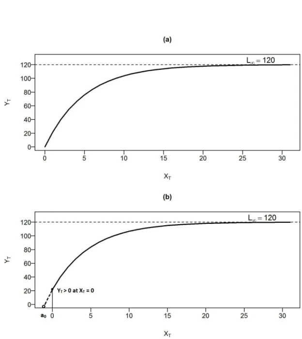
We illustrate this model in Figure 1.2 (top panel) when L∞ = 120 and k = 0.2.

This figure demonstrates that for the VonB model, fish grow more quickly when they are young, growth slows gradually as the individual fish ages, and eventually stops growing at length,L∞ = 120.

Generally, the length of a fish during its first year (age zero) is not zero, i.e.,YT >0 atXT = 0. To account for this, we use the following form of the VonB growth model,

YT(XT;L∞, ao, k) =L∞(1−e−k(XT−ao)), (1.22)

whereao <0 is the theoretical age at which a fish has zero length. In practical terms age cannot be negative, but ifYT >0 at age XT = 0 and we extrapolate the growth curve back to whenYT = 0, we obtain a negative age (see Figure 1.2, bottom panel). The VonB model (Eqn. 1.22) is used to describe the mean growth of a population whereL∞, k and a0 are the population mean growth parameters.

1.2.2 The Effect of ME in VonB Model

In reality the length of fish can usually be measured fairly accurately, however, error in measuring age (i.e. covariate ME) is very common in age-to-length data. Age reading errors may be due to 1) misinterpretation by readers of ageing structures to record growth sequence information, 2) different readers provides different age measurements. Therefore, in practice, XT is not observed, and instead of it we observe X.

(36)

The standard method used in fish stock assessments to fit VonB models, i.e., Eqn. (1.22), to data is either by nonlinear least squares (e.g. Tomilnson and Abramson, 1961 [46]) or maximum likelihood (e.g. Kimura, 1980 [29]). In both model fitting procedures YT is thought of as the expected or mean length of a fish with age X, and the fitting procedure simply selects parameter values to minimize the difference between the observed and the expected values of YT for each observed age X. This approach assumes that all the deviations between the model and the data are due to variation in length measurements. ME in age may cause bias, and we will investigate the potential magnitude of the bias using a simulation experiment.

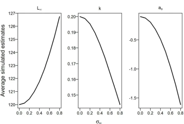
In a simulation study, we randomly generated 1000 independent datasets. For each dataset we follow the following steps:

• Step 1: We generated 1000 true ages XT from a Gamma distribution with

α = 7 andβ = 1. The pdf of the Gamma distribution with parameters αand β

is fXT(xT;α, β) = 1 βα _{Γ (}_α₎ x α−1 T e −xT_β .

• Step 2: We generated 1000 true lengths YT assuming a VonB growth model (Eqn. 1.22) using L∞ = 120, k = 0.2 and ao = −0.1 and the true age XT generated in step 1.

• Step 3: We considered the classical error model ofY defined in Eqn. (1.15) to generate 1000 observed lengths Y with σe = 0.1. We used the classical error models of X defined in Eqn. (1.16) to generate 1000 observed ages X with a range of σu values vary from 0 to 0.8.

• Step 4: For each data set we used nonlinear least squares to estimate the VonB growth parameters.

(37)

Finally, we calculate the average simulated estimates of growth model parameters. Figure 1.3 displays the change in estimates of growth parametersL∞, k, and a0 with

the magnitude of ME. The results illustrate that as the ME in age increases the change in average simulated estimates of growth parameters is substantial. When there is no ME in age, i.e., σu = 0 the average simulated estimates are the same as their corresponding true values. For example, the average estimated value of L∞ is 120.

However, as σu increases the average estimated values of L∞ increases substantially.

For instance, when σu = 0.8 then the average estimated value ofL∞ is 127, which is

very different from its true value 120. Therefore, ME in age has a substantial effect on the estimates of growth parameters.

MEs in age and length of fish have substantial consequences on estimates of growth, mortality, recruitment and yield (e.g. Bradford, 1991 [6]; Reeves, 2003 [35]). Covariate ME has long been recognized as important in fisheries science when fitting linear regression models (Schnute, 1990 [38]), stock-recruit models (Walters and Ludwig, 1981 [47]), simple biomass production models (Uhler, 1980 [48]), and growth models (e.g. Kitakado, 2000 [28], Cope and Punt, 2007 [15]), which is the focus of this study. It is difficult to estimate the ME in both age (i.e. the covariate) and length (i.e. the response) without additional information on the accuracy of at least one of these sources. An SEV model approach was used by Suh and Schafer (2001) [45]. They considered a situation where individual growth measurements were available, with error in both length and age, but also a smaller validation sample in which there were no aging errors. Such validation data are not commonly available. Cope and Punt (2007) [15] considered the more common situation in which estimates of the ageing error variance are available from multiple age measurements of a sample of fish. They suggested an SEV model with a Gamma distribution for the unobserved true ages, and they showed using simulations that this approach provided more precise estimates

(38)

1.3. ORGANIZATIONS OF SUBSEQUENT CHAPTERS 20

of VonB model parameters compared to the conventional “errors in length” nonlinear least squares method.

1.3 Organizations of Subsequent Chapters

The following chapters are organized as follows. In Chapter 2, we approximate the unobserved true age distribution using a simple Gamma distribution in an SEV VonB model to estimate the VonB model parameters. This approach is commonly used for age-to-length data (e.g. Cope and Punt, 2007 [15]). In this study, we call it the SEV VonB Gamma model. We investigate whether SEV VonB Gamma model parameter estimators are robust to misspecification of the true unobserved age distribution or not. We consider robustness (Huang, X. (2006) [53], and Huang, Stefanski, and Davidian (2006) [26]) to mean lack of bias in estimators for the parameters.

In Chapter 3, we propose an SEV VonB growth model that involves mixtures of Normal distributions for the unobserved ages, which is more robust to misspecification of the true unobserved age distribution. For our purposes, we call it the SEV VonB Normal mixture model. We compare the estimators based on the SEV VonB G-Normal mixture model with that based on the SEV VonB Gamma model in terms of large sample bias.

In Chapter 4, we extend the SEV VonB G-Normal mixture model in Chapter 3 to account for between-individual (BI) variation in growth. We assume BI variation in growth appears because individuals achieve different asymptotic sizes (L∞). Here,

we call it the SEV VonB G-Normal mixture BI model. We compare the estimators based on the SEV VonB G-Normal mixture BI model with that based on the SEV VonB Gamma BI model in terms of finite sample bias.

(39)

1.3. ORGANIZATIONS OF SUBSEQUENT CHAPTERS 21

In Chapter 5, we apply the SEV VonB G-Normal mixture BI model to the length-at-age Greenland Hailbut data in the NAFO management unit Subarea 2 + Divisions 3KLMNO provided by Dwyer et al. (2016)[17].

In Chapter 6, we conclude by summarizing the main ideas proposed in this thesis and the main results obtained.

(40)

1.4. FIGURES 22

1.4 Figures

Figure 1.1: Simulation-Extrapolation (SIMEX) estimate ˆβ1(λ) of slope parameter of

(41)

1.4. FIGURES 23

Figure 1.2: Application of the Von Bertalanffy (VonB) model for L∞ = 120, k =

0.2. The top panel illustrates the growth curve when a0 = 0, and the bottom panel

illustrates when a0 < 0. YT and XT denote the true length and true age of fish, respectively.

(42)

1.4. FIGURES 24

Figure 1.3: Average simulated values of Von Bertalanffy (VonB) parameters L∞, k

& ao estimated using the nonlinear least squares method. The measurement error variance is denoted by σu.

(43)

Chapter 2 Robustness of Structural

Errors-in-Variables Model

2.1 Introduction

In Chapter 1 we introduced the structural errors-in-variables (SEV) model. This approach was proposed to account for age ME in VonB growth models in fisheries science. Cope and Punt (2007) [15] suggested an SEV model with a Gamma distri-bution for the unobserved true ages,XT, and their results showed that this approach provided more precise estimates of VonB model parameters compared to the nonlinear least squares method.

Mohammed (2015) [32] extended the model in Cope and Punt (2007) [15] to in-clude between-individual variation in growth, but still assuming that unobserved ages have a simple Gamma distribution. The simulation studies in Mohammed (2015) [32] indicated that misspecification of the distribution of unobserved age did not result in much bias in the estimates of VonB parameters. However, we note that the age reading error variance considered in Mohammed (2015) [32] was very small. Cadigan

(44)

2.1. INTRODUCTION 26

and Campana (2016) [8] also assumed a Gamma age distribution in their hierarchi-cal modelling of growth for many fish populations, and they showed that parameter estimates did not change much when a more flexible parametric age distribution was used. Huang, Stefanski and Davidian (2006) [26] showed that when the covariate ME is low the asymptotic bias of parameter estimators is close to zero for SEV models. Therefore, potential bias is due to the joint effect of model misspecification and the magnitude of covariate ME. This was not studied much in Cope and Punt (2007) [15], Mohammed (2015) [32], or Cadigan and Campana (2016) [8].

This is the motivation for this chapter. We investigate whether SEV VonB model parameter estimators based on a simple Gamma distribution for unobserved ages are robust to misspecification of the true unobserved age distribution. We consider ro-bustness (e.g. Huang, X. (2006) [53], and Huang, Stefanski, and Davidian (2006) [26]) to mean lack of bias in estimators for the parameters of interest. In practice the true age distribution may be quite complicated, varying from unimodal to mul-timodal. The age distribution of a fish population will depend on the reproduction and survival of previous cohorts, and reproduction rates and early life-stage survival for fish are known to vary widely from year to year. This can lead to potentially complicated and multi-modal age distributions; hence, robustness to such misspecifi-cations is practically relevant. Heagerty and Kurland (2001) [23] proposed a method for evaluating large sample bias due to misspecification of the random effects distri-bution in generalized linear mixed models. A general framework to quantify the bias due to covariate ME misspecification was proposed by Hossain and Gustafson (2011) [24]. We used their approaches to compute the large sample bias in SEV VonB model parameter estimators to investigate how this is jointly affected by misspecification of the distribution of unobserved true ages and the magnitude of the ME in age.

(45)

2.2. STRUCTURAL ERRORS-IN-VARIABLES MODEL 27

2.2 Structural Errors-in-Variables Model

In this section, we investigate a method to assess the robustness of the estimates of parameters in the SEV model. Recall from Chapter 1 that the joint pdf of (Y,X) defined in Eqn. (1.20) is

fY,X(y, x;θ) = Z

fY|XT(y|xT;θR) fX|XT(x|xT;σu) fXT(xT;θE)dxT, where

1. Response Model: fY|XT(y|xT;θR) describes the relationship between Y and

XT;

2. ME Model: fX|XT(x|xT;σu) describes the relationship between X and XT; 3. Covariate Model: the true covariate XT is considered as a random variable

with pdf fXT(xT;θE). LetfT

XT(xT; ΘE) denote the true pdf ofXT andf A

XT(xT;θE) denote the assumed pdf of

XT that we use in the SEV model. If the true covariate model with pdf fXTT(xT; ΘE) is misspecified as the assumed covariate model with pdff_XA_T(xT;θE), then under such misspecificationθE may no longer be meaningful; however,θR will still be meaningful. In this chapter, our interest is in how sensitive the bias in the estimate of θR is to such misspecification.

Note that the true response model and the true ME model are the same as the corresponding assumed models because we are assuming they are correctly specified; only the covariate model is misspecified.

(46)

2.2.1 Covariate Model Correct Specification

Under the correct model, the observed data likelihood is

LT(Θ_|Y, X) = Z

fY|XT(y|xT;θR) fX|XT(x|xT;σu) f T

XT(xT; ΘE) dxT, (2.1) where Θ = (θR,ΘE). The log-likelihood function for Θ based on Y and X under correct specification is

l(Θ_|Y, X) = log_{LT(Θ _|Y, X)_}.

The score function for Θ is

S(Θ_|Y, X) = ∂ ∂Θl(Θ|Y, X) = ∂ ∂ΘL T_(Θ _|_{Y, X}₎ LT_(Θ_|_{Y, X}₎ .

The expected score function, E[S(Θ _| Y, X)], evaluated at the true parameter value

θ∗ _{of Θ is}

E[S(θ∗ _|Y, X)] = 0. (2.2)

The proof is as follows:

E[S(θ∗ _|Y, X)] = Z Z ∂ ∂ΘLT(θ∗ |Y, X) LT₍_θ∗ _|_{Y, X}₎ L T₍_θ∗ |Y, X) dy dx = Z Z _∂ ∂ΘL T₍_θ∗ |Y, X) dy dx = ∂ ∂Θ Z Z LT(θ∗ _|Y, X) dy dx = ∂ ∂Θ Z Z Z fY|XT(y|xT;θ ∗ R) fX|XT(x|xT;σu) f T XT(xT; Θ ∗ E) dxT dy dx = ∂ ∂Θ (1) = 0.

(47)

2.2.2 Covariate Model Misspecification

Under the misspecified (assumed) covariate model, the observed likelihood in Eqn. (2.1) is LA(θ _|Y, X) = Z fY|XT(y|xT;θR)fX|XT(x|xT;σu) f A XT(xT;θE) dxT, (2.3) whereθ = (θR, θE) be a (P ×1) vector. The log-likelihood function forθ based on Y and X under misspecification is

l(θ_|Y, X) = log_{LA(θ _|Y, X)_}.

The score function forθ for the misspecified model is

S(θ _|Y, X) = ∂ ∂θl(θ |Y, X) = ∂ ∂θL A₍_θ_|_{Y, X}₎ LA₍_θ _|_{Y, X}₎ .

The SEV MLE ofθ under the misspecified covariate model are the values maximizing Eqn. (2.3). Let ˆθ be the SEV MLE of θ. Hence, ˆθR is the SEV MLE ofθR.

Defineθ(σu) as a function ofσu implicitly via

E[S_{θ(σu)|Y, X}] = 0. (2.4) The expectation is taken with respect to the joint pdf of (Y,X) (Eqn. 2.1) for the correct specification of XT. Let θ(σu) = (θR(σu), θE(σu)) be the analytical solution that makes the expected score equation under misspecification (Eqn. 2.4) equal zero.

Theoretical Robustness of MLE of θR : Huang, X. (2006) [53], and Huang, Stefanski, and Davidian (2006) [26] proposed a method to study the robustness to

(48)

model specification of XT. For studying robustness, we assume that ME exists with known variance σu and that the unknown pdf of XT is possibly misspecified. The SEV MLE ˆθR is robust if

θR(σu) is approximately equal to θ_R∗ for σu ≥0,

where θ_R∗ is the true parameter value that makes the correctly specified mean score function equal to zero. Therefore, the asymptotic bias in the SEV MLE of θR that arises due to covariate model misspecification is

Asymptotic Bias(ˆθR) = θR(σu)−θR∗. (2.5) The main difficulty in finding the asymptotic bias of ˆθR is finding the analytical solutionθR(σu) when there is no closed form of Eqn. (2.4). Therefore, to approximate the solution of θ(σu) one idea is to generate a large sample of size n and apply the large sample theory of estimation. The large sample estimation process for θ(σu) is described below.

2.2.3 Estimating Method of the SEV Model Parameters

Let D = (Yi, Xi)ni=1 denote independent realizations from the ME models defined in

Eqns. (1.15) and (1.16) andDi = (Yi, Xi) be the ith realization. By the law of large numbers we have 1 n n X i=1 S_{θ(σu)_|Di} p →E[S_{θ(σu)_|Y, X_}],

(49)

in probability when n is large. Therefore, for large sample estimation of θ(σu) we need to solve

n X

i=1

S_{θ(σu)_|Di}= 0, (2.6) for a large sample of sizen. Eqn. (2.6) is the estimating equation forθ(σu) under the misspecified model. Let ˜θ(σu) be the solution to the estimating Eqn. (2.6) for largen. We used the Newton-Raphson (N-R) iterative method to solve the estimating Eqn. (2.6) forθ(σu), where at any particular iteration (r+1) we have

˜

θ(r+1)(σu) = ˜θ(r)(σu)₋[I_{θ˜(r)(σu)_}]−1[S_{θ˜(r)(σu)_}], (2.7) whereS_{θ˜(r)(σu)_}is a (P_×1) score vector andI_{θ˜(r)(σu)}is a (P×P) Hessian matrix at the rth _{iteration. The j}th _{element of} _S_{_θ˜(r)₍_σ_u)_}_is

Sj{θ˜(r)(σu)}= n X i=1 Sj{θ˜(r)(σu)|Di}= n X i=1 ∂ ∂θj l_{θ(σu)_|Di} θ(σu)=˜θ(r)(σu) , (2.8)

and the (k, j)th _{element of}_I_{_θ˜(r)₍_σ_u)_}_is

Ik,j{θ˜(r)(σu)}= n X i=1 Ik,j{θ˜(r)(σu)|Di}= n X i=1 ∂2 ∂θk∂θj l_{θ(σu)_|Di} θ(σu)=˜θ(r)(σu) , (2.9)

for j, k = 1,2, . . . ,P. Evaluation of the terms in Eqns. (2.8)-(2.9) requires evaluation of integrals with no closed form except in the case of the linear regression model. Therefore, numerical integration is required. The estimation procedure discussed in Hossain and Gustafson (2011) [24] is as follows:

1. Generate a sample of the D= (Yi, Xi)n_i=1 using Eqns. (1.15) and (1.16);

2. Integrate out theXT numerically in order to evaluateS{θ(σu)|Di}andI{θ(σu)|

(50)

3. Use the N-R iterative method discussed in the Eqn. (2.7) to find ˜θ(σu).

Large Sample Bias of MLE of θR : Let ˜θ(σu) be the numerically approximating

θ(σu) of Eqn. (2.6) for large n. The large sample bias in the SEV MLE ˆθR under covariate model misspecification is

Bias(ˆθR) = ˜θR(σu)₋θ∗_R,

which is a numerical approximation of the asymptotic bias defined in Eqn. (2.5). Therefore, the SEV MLE for θR, i.e., ˆθR is robust if

˜

θR(σu) approximately equal to θR∗ forσu ≥0.

2.2.4 Example: Assessing Bias due to Covariate Model

Mis-specification in a Simple Linear Model

Huang, Stefanski, and Davidian (2006) [26] investigated the bias in the estimates of the parameters in a simple linear model due to covariate model misspecification. We have reproduced their results to check our bias estimation procedure for the SEV model. The linear model specifies Y as a function ofXT,

Y =βo+β1XT +ǫ,

with β0 and β1 are the intercept and slope parameters, respectively. Suppose, XT is measured with the classical ME model,

(51)

Assume that ǫ and U are N(0, σ_e2) and N(0, σ_u2), respectively. 1. Response Model: The Normal pdf of Y given XT is

fY|XT(y|xT;θR) = 1 σe √ 2πe −(y−η(xT_;_β 0,β1))2/2σ2e_, _(2.10) where η(xT_;_β 0, β1) =βo+β1xT and θR= (βo, β1, σe2). 2. ME Model: The Normal pdf of X given XT is

fX|XT(x|xT;σu) = 1 σu √ 2πe −(x−xT)2/2σ2u_. _(2.11) 3. Covariate Model: The assumed Normal pdf of XT is

f_XA_T(xT, θE) = 1

µ√2πe

−(xT−µ)2/2µ2_. _(2.12) where the parameter, θE = µ. The mean, E(XT) = µ, variance, V(XT) = µ2, and the coefficient of variation, CV(XT)= 1.

To estimate the parameters of interest (β0 and β1) we follow the estimating method

discussed in Section 2.2.3. We used the simulation procedure described below to compute the large sample bias in the SEV MLE ofβ0 and β1.

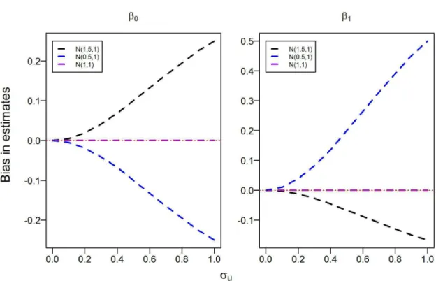
A large random sample (n = 50,000) of responses Y were generated with pa-rameters fixed at β0 = 0, β1 = 1 and σe = 1. Three true distributions of XT were investigated: N(0.5,1), N(1,1), and N(1.5,1). When the true distribution of XT is

N(1,1) then the assumed model N(µ, µ2) is correctly specified, while for the other two cases the assumed model is incorrect. Figure 2.1 displays the bias in the estimates ofβ0 and β1 againstσu for three true distributions of XT, two of which were misspec-ified asN(µ, µ2_{). The misspecification and lack of flexibility in modelling} _X _results

(52)

2.3. SEV VONB MODEL 34

in bias in the estimates of β0 and β1 that increase in magnitude with σu. Virtually

identical results were provided by Huang, Stefanski and Davidian (2006) [26].

2.3 SEV VonB Model

Let Y be the measured length of a fish, YT be the unknown true length, XT be the unobserved true age, and X be the observed age. For simplicity we assume that measurements of both length and age of fish are continuous similar to Cope and Punt (2007) [15]. The VonB growth model specifiesYT as a function of XT,

YT(XT;L∞, ao, k) =L∞(1−e−k(XT−ao)).

The parameter L∞ is the asymptotic length (asXT → ∞) at which the growth rate is zero, k is the growth rate parameter, and ao < 0 is the theoretical age at which a fish has zero length. We assume that the observed length (Y) and age of fish (X) have independent multiplicative MEs,

Y =YT(XT;L∞, ao, k) eǫ, (2.13)

X =XT eU, (2.14)

whereǫisN(0, σ2_e) andUisN(0, σ_u2). SinceUisN(0, σ2_u),eUis a Lognormal(0, σu) dis-tribution. The coefficient of variation of a Lognormal(0, σu) distribution is

√

eσ2

u−1, which is approximatelyσu whenσu is small. Therefore, e.g. σu = 0.3 will be regarded as 30 percent ME variance in age.

We assume multiplicative ME in length because in practice errors will be smaller for small fish compared to larger sizes. Errors in age will also usually increase with

(53)

age because it is more difficult to count annual otolith growth increments for older fish; therefore, the multiplicative error in age is valid as described in Cope and Punt (2007) [15] and Cadigan and Campana (2016)[8].

1. Length Model: The Lognormal pdf of Y given XT is

fY|XT(y|xT;θR) = 1 yσe √ 2πe −(log(y)−η(xT;L∞,k,ao))2/2σ2e_, (2.15) where η(xT;L∞, k, ao) = log{L∞(1−e−k(xT−ao))} and θR= (L∞, k, ao, σ2e). 2. ME Model: The Lognormal pdf of X given XT is

fX|XT(x|xT;σu) = 1 xσu √ 2πe −(log(x)−log(xT))2/2σ2u_. _(2.16) 3. Age Model: The assumed pdf of XT is Gamma,

f_XA_T(xT;θE) = 1 βα _{Γ (}_α₎ x α−1 T e −xT_β _, (2.17)

where the parameter vector θE = (α, β). The mean is E(XT) = αβ and the variance is V(XT) = αβ2.

In this study, we called an SEV VonB model with a simple Gamma distribution for unobserved ages a SEV VonB Gamma model. For simplicity, we assumed σe was known. To estimate the parameters, i.e. θ= (L∞, k, ao, α, β),we follow the estimating method discussed in Section 2.2.3. The score vector and Hessian matrix ofθ for this model are provided in Appendix A. The R procedure “integrate” is used to integrate out theXT numerically in order to evaluate the score vector and Hessian matrix ofθ. In the next section, we conduct a simulation study to investigate the impact of mis-specifying the true unobserved age distribution as Gamma when it is actually

(54)

something else, like a Lognormal or mixture of distributions.

2.3.1 Simulation Design and Settings

The response Y is generated assuming a VonB growth model (Eqn. 2.13) with the parameters fixed at L∞ = 120, k = 0.2, ao = −0.1 and σe = 0.1. We assume that only the true unobserved age distribution is misspecified. For all simulation setups we considerσu varies from 0 to 0.3. When σu = 0, there is no ME in age. We use a sample of sizen = 50,000 for studying the bias in the estimates of θR= (L∞, k, ao).

2.3.2 Simulation Design 1: Lognormal versus Gamma

Distri-bution for True Age

The true distribution of unobserved age XT is generated from a Lognormal(µ, σ) distribution with pdf f_XT_T(xT; ΘE) = 1 xT σ √ 2πe −(log(xT)−µ)2/2σ2_. _(2.18) The parameter vector includes ΘE = (µ, σ). The mean is E(XT) =eµ+

σ2

2 , the variance

is V(XT) = (eσ

2

−1)e2µ+σ2

, the coefficient of variation is CV(XT) =

√

eσ2

−1, and the skewness is Sk = (eσ2

+ 2)√eσ2

−1. We consider different degrees of skewness and heavy tailedness for the distribution of XT. Different simulation settings for the true unobserved age distribution of fish are:

1. E(XT) = 4, CV(XT) = 0.5; therefore,µ = 1.275, σ = 0.4723 and Sk = 1.6; 2. E(XT) = 7, CV(XT) = 0.5; therefore,µ = 1.834, σ = 0.4723 and Sk = 1.6; 3. E(XT) = 10, CV(XT) = 0.5; therefore, µ = 2.2,σ = 0.4723 and Sk = 1.6;

(55)

4. E(XT) = 4, CV(XT) = 1.5; therefore,µ = 0.7946, σ = 1.085 and Sk = 7.9; 5. E(XT) = 7, CV(XT) = 1.5; therefore,µ = 1.35,σ = 1.085 and Sk = 7.9; 6. E(XT) = 10, CV(XT) = 1.5; therefore, µ = 1.713, σ = 1.085 and Sk = 7.9.

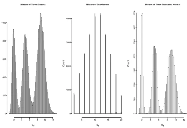
Figure 2.2 illustrates the simulated true ages. Cases 1-3 represent situations where the Lognormal distributions have less heavy tails and cases 4-6 have heavier tails. Cases 1-3 and 4-6 are contrasting situations where the levels of skewness are different for the same corresponding mean age. The Gamma distribution is expected to pick up the shape of the true unobserved age distributions in cases like 4-6. Cases 1-3 are considered to examine whether light tails in the age distribution are a factor contributing to estimator bias.

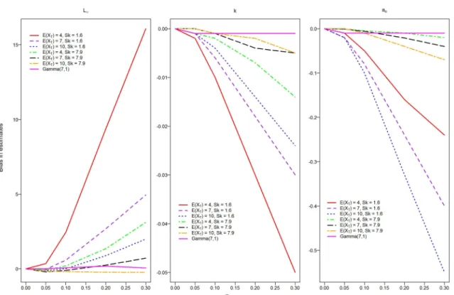
As shown in Figure 2.3, in case of correct specification, i.e., when the true dis-tribution of XT follows Gamma(α = 7, β = 1), there is little bias in the estimators of L∞, k and ao. However, mis-specifying the distribution of XT as Gamma (when it was actually Lognormal) may result in large bias in estimators of L∞, k and ao. When there is no ME in age, i.e. σu = 0, all the estimated values are about the same as the true values of the corresponding parameters irrespective of the different levels of skewness in the true age distribution. The estimates of the VonB growth parameters are fairly close to their true values whenσu is less than 5 percent. Hence, misspecification of the true age distribution does not cause much bias when ME in age is low. However, as σu increases the bias of these estimators increases substantially in cases like 1-2 where skewness is comparatively small. Notice that across all the situationsL∞ is overestimated while k and ao are underestimated. The bias inL∞ is

negatively correlated with the bias ink, which is expected as described in (e.g. Quinn and Deriso, 1999 [51]). Interestingly, when skewness increases to 7.9 from 1.6, the bias inL∞, k and ao becomes low.

(56)

It is well known that a broad range of ages is required to estimate VonB model parameters reliably. This should include young fish whose growth rates provide more direct information about k, and old fish that provide information about the asymp-totic size,L∞. Otherwise, there may be confounding between k and L∞. To further

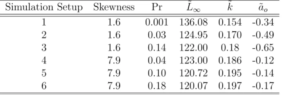
explore how the distribution of ages may affect bias, we computed the proportion of large fish (Y > 0.95L∞) and investigated the relationship of this proportion with

bias. LetX0.95L∞ be the age at which the length of a fish is 95 percent of L∞= 120.

Let Pr denote the probability of the event (X >X0.95L∞), which is an indicator of

the proportion of old aged fish in the population. Table 2.1 demonstrates that when the skewness of the Lognormal age distributions is the same as the proportion of old aged population Pr increases the bias in the estimates ofL∞, k and ao decreases. For example, in cases like 1-3 where the skewness is 1.6, the proportion of old aged fish increases from 0.001 to 0.14, and the bias in the estimates ofL∞ andk decreases

sub-stantially as Pr increases. Therefore, the percentage of old aged fish in the population seems to be a factor contributing to the bias in the estimates of L∞ and k.

The results from Table 2.2 are based on two cases where the true unobserved age distributions are Lognormal with the same mean, 4. The proportion of old aged fish in the population is 0.001 for both cases, however, the level of skewness is different. Table 2.2 indicates that when the skewness increases from 1.63 to 2.67 the change in bias in the estimates is substantial. It implies that when the percentage of old aged fish in the population is small the bias in the estimates are high irrespective of the level of skewness increases.

The results from Table 2.3 are based on cases where the percentage of old aged fish is 4 percent, and skewness increases from 7.86 to 13.97. The bias in the estimates ofL∞, k, andao are low as skewness increases. It implies that when the percentage of old aged fish in the population is large the bias in the estimates are low irrespective

Sensitivity to model misspecification of the Von Bertanlanffy grown model with measurement error in age